On Convergence Analysis and Analytical Solutions of the Conformable Fractional Fitzhugh–Nagumo Model Using the Conformable Sumudu Decomposition Method

Abstract

The current article studied a nonlinear transmission of the nerve impulse model, the Fitzhugh–Nagumo (FN) model, in the conformable fractional form with an efficient analytical approach based on a combination of conformable Sumudu transform and the Adomian decomposition method. Convergence analysis and error analysis were also carried out based on the Banach fixed point theory. We also provided some examples to support our results. The results obtained revealed that the presented approach is very fantastic, effective, reliable, and is an easy method to handle specific problems in various fields of applied sciences and engineering. The Mathematica software carried out all the computations and graphics in this paper.

1. Introduction

Numerous nonlinear fractional models have paramount importance in applied science and engineering like fluid mechanics, geophysical fluid mechanics, fluid mechanics, thermodynamic, plasma physics, relaxation vibrations, heat transfer, and optics [1,2,3,4]. For instance, The fractional Fitzhugh–Nagumo model (FN) is an important nonlinear model for describing the transmission of thermal energy in thermodynamics, circuit theory, biology, and in the area of population genetics [5,6,7].

$$\begin{array}{c}\hfill \frac{{\partial }^{\alpha }\phi }{\partial t^{\beta }}-\frac{{\partial }^2\phi }{\partial x^2}=\left(1+\delta \right){\phi }^2-{\phi }^3-\delta \phi ,\alpha \in \left(0,1\right],\end{array}$$

(1)

here, $\varphi =\varphi \left(x,t\right)$, $\delta$, is an arbitrary constant. For $\alpha =1$, Equation (1) reduces to classical Fitzhugh–Nagumo equation

$$\begin{array}{c}\hfill \frac{\partial \varphi }{\partial t}-\frac{{\partial }^2\varphi }{\partial x^2}=\left(1+\delta \right){\varphi }^2-{\varphi }^3-\delta \varphi ,\end{array}$$

(2)

and for $\delta =-1$, Equation (2) converts into the famous Newell–Whitehead partial differential equation. Equation (2) was first introduced by Hodgkin and Huxley and obtained at first to model the transmission of nerve impulses. In the last decades, many numerical and analytical techniques were applied to the classical and fractional FN equations to find their approximate and analytical solutions, some of which are; homotopy analysis method [8], first integral method [9], haar wavelet method [10], Hirota method [11], Jacobbi elliptic function method [12] Adomian decomposition method [13] wavelet method [14], q-homotopy analysis method [15], finite element method [16], modified trial equation method [17], Pseudospectral method [18], and so on.

During the last few years, the conformable fractional derivative and integral have received much attention, and many applications have been remodeled using their definitions. Moreover, they have many exciting advantages that make them more comfortable and more flexible than the definitions of other fractional derivatives, especially Caputo and Reimann Liouville derivatives. Among these advantages, the conformable fractional derivative (CFD) satisfies all ordinary calculus concepts such as product, quotient, Rolle’s theorem, and mean-value theorem, chain rules. A non-differentiable function can be $\mu$-differentiable in terms of conformable sense [19,20,21]. FN has been studied very extensively and, there is pervasive literature available of the solutions of FN differential equations of fractional order, where the fractional derivatives are in terms of Caputo or Reimann–Liouville. Nevertheless, there is very little or no work available on solving the FN involving conformable fractional derivatives. Motivated by those mentioned above, we feel compelled to solve the FN model in the form of conformable space.

The conformable form of FN Equation (2) is given by

$$\begin{array}{c}\hfill \frac{{\partial }^{\mu }\varphi }{\partial t^{\mu }}-\frac{{\partial }^{2\lambda }\varphi }{\partial x^{2\lambda }}=\left(1+\delta \right){\varphi }^2-{\varphi }^3-\delta \varphi ,\end{array}$$

(3)

with the initial condition

$$\begin{array}{c}\hfill \varphi \left(x,0\right)=\psi \left(\frac{x^{\lambda }}{\lambda }\right).\end{array}$$

(4)

where, $\varphi =\varphi \left(\frac{x^{\lambda }}{\lambda }.\frac{t^{\mu }}{\mu }\right)$, and $\lambda ,\mu$ are the parameters defining the structure of the CFD $\left(0<\lambda ,\mu \le 1\right)$.

In this paper, we develop the conformable Sumudu decomposition method (CSDM) application to study the conformable fractional FN equation. The CSDM is a modified algorithm based on the combination of the Adomian [22] decomposition scheme and conformable Sumudu transform method [23]. The remaining part of this article is structured as follows: In the next section, we present some basic definitions of the conformable fractional derivatives and the conformable Sumudu transform. In Section 3, the main idea of the proposed method is described. The convergence of the solution is discussed and proved in Section 4. In Section 5, we devote ourselves to applying the (CSDM) for conformable fractional FN equations. In Section 6, we discuss the numerical results and illustrate the accuracy and efficiency of the CSDM. Conclusions are outlined in Section 7.

2. Preliminaries

In this segment, we briefly recall some fundamental theories and formulas related to the conformable fractional derivative (CFD) and conformable Summudu transform (CST) which can be found in [23,24,25,26,27,28,29,30,31].

Definition 1.

Let $\mu \in \left(n,n+1\right],$ $n\in \mathrm{N}$, and $\varphi :\mathrm{R}\times \left(0,\infty \right)\to \mathrm{R}$, be an $n-\mathrm{differentiable}$ function at $x,t>0$, then the CFD of order μ of the function $\varphi \left(x,t\right)$ is given by

$$\begin{array}{c}\hfill \frac{{\partial }^{\mu }\varphi \left(x,t\right)}{\partial t^{\mu }}=\underset{\nu \to 0}{lim}\frac{{\varphi }^{\left(⌈\mu ⌉-1\right)}\left(x,t+\nu t^{\left(⌈\mu ⌉-\mu \right)}\right)-{\varphi }^{\left(⌈\mu ⌉-1\right)}\left(x,t\right)}{\nu }.\end{array}$$

Definition 2.

Let $\lambda \in \left(m,m+1\right],$$n\in \mathrm{N}$, and $\varphi :\mathrm{R}\times \left(0,\infty \right)\to \mathrm{R}$, be an $m-\mathrm{differentiable}$ function at $x,t>0$, then the CFD of order λ of the function $\varphi \left(x,t\right)$ is given by

$$\begin{array}{c}\hfill \frac{{\partial }^{\lambda }\varphi \left(x,t\right)}{\partial x^{\lambda }}=\underset{\zeta \to 0}{lim}\frac{{\varphi }^{\left(⌈\lambda ⌉-1\right)}\left(x+\zeta x^{\left(⌈\lambda ⌉-\lambda \right)},t\right)-{\varphi }^{\left(⌈\lambda ⌉-1\right)}\left(x,t\right)}{\zeta }.\end{array}$$

Theorem 1.

Let $\lambda ,\mu \in \left(n,n+1\right]$, $n\in \mathrm{N}$. If ϕ is $\lambda ,\mathrm{and}\mu$-differentiable at $x,t>0$, then

$$\begin{array}{cc}\hfill & \frac{{\partial }^{\lambda }\varphi \left(x,t\right)}{\partial x^{\lambda }}=x^{{}^{\left(⌈\lambda ⌉-\lambda \right)}}\frac{{\partial }^{⌈\lambda ⌉}\varphi \left(x,t\right)}{\partial x^{⌈\lambda ⌉}},\hfill \\ \hfill & \frac{{\partial }^{\mu }\varphi \left(x,t\right)}{\partial t^{\mu }}=t^{{}^{\left(⌈\mu ⌉-\mu \right)}}\frac{{\partial }^{⌈\mu ⌉}\varphi \left(x,t\right)}{\partial t^{⌈\mu ⌉}}.\hfill \end{array}$$

In the following example, we introduce the CFD of some certain functions.

Example 1.

Let $0<\lambda ,\mu \le 1,\mathrm{and}c,d,m,n,\mathrm{and},k\in \mathrm{R}$, then, we have the following

1.

$\frac{{\partial }^{\lambda }\left(k\right)}{\partial x^{\lambda }}=\frac{{\partial }^{\lambda }\left(k\right)}{\partial x^{\lambda }}=0,\forall \mathrm{constant}\mathrm{functions}\varphi \left(x,t\right)=k.$

2.

$\frac{{\partial }^{\lambda }}{\partial x^{\lambda }}\left(k{\left(\frac{x^{\lambda }}{\lambda }\right)}^n{\left(\frac{t^{\mu }}{\mu }\right)}^m\right)=nk{\left(\frac{x^{\lambda }}{\lambda }\right)}^{n-\nu }{\left(\frac{t^{\mu }}{\mu }\right)}^m.$

3.

$\frac{{\partial }^{\lambda }\left(k\right)}{\partial x^{\lambda }}\left(k{\left(\frac{x^{\lambda }}{\lambda }\right)}^n{\left(\frac{t^{\mu }}{\mu }\right)}^m\right)=mk{\left(\frac{x^{\lambda }}{\lambda }\right)}^r{\left(\frac{t^{\mu }}{\mu }\right)}^{m-\beta }.$

4.

$\frac{{\partial }^{\lambda }}{\partial x^{\lambda }}\left(e^{c\left(\frac{x^{\lambda }}{\lambda }\right)+d\left(\frac{t^{\mu }}{\mu }\right)}\right)=c{e}^{{}^{c\left(\frac{x^{\lambda }}{\lambda }\right)+d\left(\frac{t^{\mu }}{\mu }\right)}}.$

5.

$\frac{{\partial }^{\lambda }}{\partial x^{\lambda }}\left(e^{c\left(\frac{x^{\lambda }}{\lambda }\right)+d\left(\frac{t^{\mu }}{\mu }\right)}\right)=d{e}^{{}^{c\left(\frac{x^{\lambda }}{\lambda }\right)+d\left(\frac{t^{\mu }}{\mu }\right)}}.$

Definition 3.

Let $0<\mu \le 1$, and$\varphi :\mathrm{R}\times \left(0,\infty \right)\to \mathrm{R}$. Then the CST w.r.t (t) of order μ is defined by

$$\begin{array}{c}\hfill S_t^{\mu }\left(\varphi \left(x,t\right):u\right)={\int }_0^{\infty }\varphi \left(x,ut\right)e^{-\frac{t^{\mu }}{\mu }}{t}^{\mu -1}dt.\end{array}$$

Example 2.

Let $\varpi ,n\in \mathrm{R}$ and $\mu \in \left(0,1\right]$, then the CST for of specific functions is calculated by:

1.

$S_t^{\mu }\left(\varpi \right)=\varpi ,\forall \mathrm{constant}\mathrm{functions}\varphi \left(t\right)=\varpi .$

2.

$S_t^{\mu }\left({\left(\frac{t^{\mu }}{\mu }\right)}^n\right)=\Gamma (s+1)u^n,$

3.

$S_t^{\mu }\left(e^{\frac{\varpi t^{\mu }}{\mu }}\right)=\frac{1}{\left(1-\varpi u\right)},\varpi u>1.$

4.

$S_t^{\mu }\left(sin\left(\frac{\varpi t^{\mu }}{\mu }\right)\right)=\frac{\varpi }{\left(1+{\varpi }^2{u}^2\right)},\left|\varpi \right|u>1.$

5.

$S_t^{\mu }\left(cos\left(\frac{\varpi t^{\mu }}{\mu }\right)\right)=\frac{1}{\left(1+{\varpi }^2{u}^2\right)},\left|\varpi \right|u>1.$

Theorem 2.

The CST of $\frac{{\partial }^{n\mu }\varphi \left(x,t\right)}{\partial t^{n\mu }}$ w.r.t (t) can be calculated as

$$\begin{array}{c}\hfill S_t^{\mu }\left(\frac{{\partial }^{n\mu }\varphi \left(x,t\right)}{\partial t^{n\mu }}\right)=\frac{S_t^{\mu }\left(\varphi \left(x,t\right)\right)-\varphi \left(x,0\right)}{u^n}-\sum _{i=1}^{n-1}{u}^{i-n}\left(\frac{{\partial }^{i\mu }\varphi \left(x,0\right)}{\partial t^{i\mu }}\right).\end{array}$$

(5)

In particular,

$$\begin{array}{cc}\hfill & S_t^{\mu }\left(\frac{{\partial }^{\mu }\varphi \left(x,t\right)}{\partial t^{\mu }}\right)=\frac{S_t^{\mu }\left(\varphi \left(x,t\right)\right)-\varphi \left(x,0\right)}{u},\hfill \\ \hfill & S_t^{\mu }\left(\frac{{\partial }^{2\mu }\varphi \left(x,t\right)}{\partial t^{2\mu }}\right)=\frac{S_t^{\mu }\left(\varphi \left(x,t\right)\right)-\varphi \left(x,0\right)}{u^2}-\frac{1}{u}\frac{{\partial }^{\mu }\varphi \left(x,0\right)}{\partial t^{\mu }}.\hfill \end{array}$$

3. Analysis of (CSDM)

Herein, we demonstrate the proposed approach by considering the general form of the nonlinear conformable fractional equation.

$$\begin{array}{c}\hfill \frac{{\partial }^{\mu }\varphi }{\partial t^{\mu }}=\frac{{\partial }^{2\lambda }\varphi }{\partial x^{2\lambda }}-\delta \varphi +N\left(\varphi \right),\end{array}$$

(6)

with initial condition

$$\begin{array}{c}\hfill \varphi \left(x,0\right)=\psi \left(\frac{x^{\lambda }}{\lambda }\right).\end{array}$$

(7)

Taking the CST $S_t^{\mu }$, of Equation (6), we have

$$\begin{array}{c}\hfill S_t^{\mu }\left[\left.\frac{{\partial }^{\mu }\varphi }{\partial t^{\mu }}\right]=S_t^{\mu }\left[\frac{{\partial }^{2\lambda }\varphi }{\partial x^{2\lambda }}-\delta \varphi +N\left(\varphi \right)\right.\right],\end{array}$$

(8)

using the differentiation property of the (CST), we obtain

$$\begin{array}{c}\hfill S_t^{\mu }\left(\varphi \left(\frac{x^{\lambda }}{\lambda },\frac{t^{\mu }}{\mu }\right)\right)=\varphi \left(\frac{x^{\lambda }}{\lambda },0\right)+u{S}_t^{\mu }\left[\frac{{\partial }^{2\lambda }\varphi }{\partial x^{2\lambda }}-\delta \varphi +N\left(\varphi \right)\right].\end{array}$$

(9)

Transforming the inverse CST both sides of Equation (9), we get

$$\begin{array}{c}\hfill \varphi \left(\frac{x^{\lambda }}{\lambda },\frac{t^{\mu }}{\mu }\right)=\varphi \left(\frac{x^{\lambda }}{\lambda },0\right)+S_t^{-1}\left(u{S}_t^{\mu }\left[\frac{{\partial }^{2\lambda }\varphi }{\partial x^{2\lambda }}-\delta \varphi +N\left(\varphi \right)\right]\right).\end{array}$$

(10)

Now, Adomian solution is

$$\begin{array}{c}\hfill \varphi \left(\frac{x^{\lambda }}{\lambda },\frac{t^{\mu }}{\mu }\right)=\sum _{j=0}^{\infty }{\varphi }_j\left(\frac{x^{\lambda }}{\lambda },\frac{t^{\mu }}{\mu }\right),\end{array}$$

(11)

and, we decompose the nonlinear term according to the following series of the Adomian polynomials

$$\begin{array}{c}\hfill N\left(\varphi \right)=\sum _{j=0}^{\infty }{A}_j,\end{array}$$

(12)

where,

$$\begin{array}{c}\hfill A_j\left({\varphi }_0,{\varphi }_1,\dots ,{\varphi }_n\right)=\frac{1}{j!}{\left[\frac{d^j}{d{\omega }^j}\left[N\sum _{j=0}^{\infty }\left({\omega }^j{\varphi }_j\right)\right]\right]}_{\omega =0}.\end{array}$$

Substituting Equations (11) and (12) in (10), we get

$$\begin{array}{c}\hfill \sum _{j=0}^{\infty }{\varphi }_j\left(\frac{x^{\lambda }}{\lambda },\frac{t^{\mu }}{\mu }\right)=\psi \left(\frac{x^{\lambda }}{\lambda }\right)+S_t^{-1}\left(u{S}_t^{\mu }\left[\frac{{\partial }^{2\lambda }\left({\sum }_{j=0}^{\infty }{\varphi }_j\left(\frac{x^{\lambda }}{\lambda },\frac{t^{\mu }}{\mu }\right)\right)}{\partial x^{2\lambda }}-\delta \sum _{j=0}^{\infty }{\varphi }_j\left(\frac{x^{\lambda }}{\lambda },\frac{t^{\mu }}{\mu }\right)+\sum _{j=0}^{\infty }{A}_j\right]\right),\end{array}$$

(13)

comparing both sides of (13), we get

$$\begin{array}{cc}\hfill & {\varphi }_0\left(\frac{x^{\lambda }}{\lambda },\frac{t^{\mu }}{\mu }\right)=\psi \left(\frac{x^{\lambda }}{\lambda }\right),\hfill \\ \hfill & {\varphi }_{j+1}\left(\frac{x^{\lambda }}{\lambda },\frac{t^{\mu }}{\mu }\right)=S_t^{-1}\left(u{S}_t^{\mu }\left[\frac{{\partial }^{2\lambda }\left({\varphi }_j\left(\frac{x^{\lambda }}{\lambda },\frac{t^{\mu }}{\mu }\right)\right)}{\partial x^{2\lambda }}-\delta {\varphi }_j\left(\frac{x^{\lambda }}{\lambda },\frac{t^{\mu }}{\mu }\right)+A_j\right]\right),j=0,1,2,\cdots .\hfill \end{array}$$

(14)

4. Convergence Analysis

In this segment, we discuss the sufficient condition that guarantees the CFN equation’s unique solution, and we present the proposed method’s error analysis.

We follow [32,33] to introduce next theorem.

Theorem 3.

For $0<\vartheta <1$, where $\vartheta =\left({\epsilon }_1+{\epsilon }_2\right)\left(\frac{t^{\mu }}{\mu }\right)$ Equation (14) has a unique solution.

Proof. 

Let $\Im =\left(C[0,T],∥.∥\right)$ be the Banach space of all continuous functions, we define a mapping $G:\Im \to \Im$ as follows

$$\begin{array}{c}\hfill {\varphi }_{j+1}\left(\frac{x^{\lambda }}{\lambda },\frac{t^{\mu }}{\mu }\right)=\psi \left(\frac{x^{\lambda }}{\lambda }\right)+S_t^{-1}\left(u{S}_t^{\mu }\left[R\left({\varphi }_j\left(\frac{x^{\lambda }}{\lambda },\frac{t^{\mu }}{\mu }\right)\right)+N\left({\varphi }_j\left(\frac{x^{\lambda }}{\lambda },\frac{t^{\mu }}{\mu }\right)\right)\right]\right),j=0,1,2,\cdots ,\end{array}$$

where $R\left(\varphi \left(\frac{x^{\lambda }}{\lambda },\frac{t^{\mu }}{\mu }\right)\right)=\left(\frac{{\partial }^{2\lambda }}{\partial x^{2\lambda }}-\delta \right)\left(\varphi \left(\frac{x^{\lambda }}{\lambda },\frac{t^{\mu }}{\mu }\right)\right),$ Now suppose $R\mathrm{and}N$ are also Lipschitzian with $∥R\varphi -R\tilde{\varphi }∥<{\epsilon }_1∥\varphi -\tilde{\varphi }∥,\mathrm{and}∥N\varphi -N\tilde{\varphi }∥<{\epsilon }_2∥\varphi -\tilde{\varphi }∥$, where ${\epsilon }_1$ and, ${\epsilon }_3$ are Lipschitz constants $\varphi$ and, $\tilde{\varphi }$ are different functions.

$$\begin{array}{cc}\hfill ∥G\varphi -G{\tilde{\varphi }}_j∥& =\left|S_t^{-1}\left(u{S}_t^{\mu }\left[R\left({\varphi }_j\left(\frac{x^{\lambda }}{\lambda },\frac{t^{\mu }}{\mu }\right)\right)+N\left({\varphi }_j\left(\frac{x^{\lambda }}{\lambda },\frac{t^{\mu }}{\mu }\right)\right)\right]\right)-S_t^{-1}\left(u{S}_t^{\mu }\left[R\left({\tilde{\varphi }}_j\left(\frac{x^{\lambda }}{\lambda },\frac{t^{\mu }}{\mu }\right)\right)+N\left({\tilde{\varphi }}_j\left(\frac{x^{\lambda }}{\lambda },\frac{t^{\mu }}{\mu }\right)\right)\right]\right)\right|\hfill \\ \hfill & \le \underset{t\in [0,T]}{max}\left|S_t^{-1}\left(u{S}_t^{\mu }\left[R\left({\varphi }_j\left(\frac{x^{\lambda }}{\lambda },\frac{t^{\mu }}{\mu }\right)\right)-R\left({\tilde{\varphi }}_j\left(\frac{x^{\lambda }}{\lambda },\frac{t^{\mu }}{\mu }\right)\right)\right]\right)+S_t^{-1}\left(u{S}_t^{\mu }\left[N\left({\varphi }_j\left(\frac{x^{\lambda }}{\lambda },\frac{t^{\mu }}{\mu }\right)\right)-N\left({\tilde{\varphi }}_j\left(\frac{x^{\lambda }}{\lambda },\frac{t^{\mu }}{\mu }\right)\right)\right]\right)\right|\hfill \\ \hfill & \le \underset{t\in [0,T]}{max}\left[{\epsilon }_1{S}_t^{-1}\left(u{S}_t^{\mu }\left[\left|\left({\varphi }_j\left(\frac{x^{\lambda }}{\lambda },\frac{t^{\mu }}{\mu }\right)\right)-{\tilde{\varphi }}_j\left(\frac{x^{\lambda }}{\lambda },\frac{t^{\mu }}{\mu }\right)\right|\right]\right)+{\epsilon }_2{S}_t^{-1}\left(u{S}_t^{\mu }\left[\left|\left({\varphi }_j\left(\frac{x^{\lambda }}{\lambda },\frac{t^{\mu }}{\mu }\right)\right)-{\tilde{\varphi }}_j\left(\frac{x^{\lambda }}{\lambda },\frac{t^{\mu }}{\mu }\right)\right|\right]\right)\right]\hfill \\ \hfill & \le \underset{t\in [0,T]}{max\left({\epsilon }_1+{\epsilon }_2\right)}\left[S_t^{-1}\left(u{S}_t^{\mu }\left[\left|\left({\varphi }_j\left(\frac{x^{\lambda }}{\lambda },\frac{t^{\mu }}{\mu }\right)\right)-{\tilde{\varphi }}_j\left(\frac{x^{\lambda }}{\lambda },\frac{t^{\mu }}{\mu }\right)\right|\right]\right)\right]\hfill \\ \hfill & \le \underset{t\in [0,T]}{max\left({\epsilon }_1+{\epsilon }_2\right)}\left[S_t^{-1}\left(u{S}_t^{\mu }\left[∥w\left({\varphi }_j\left(\frac{x^{\lambda }}{\lambda },\frac{t^{\mu }}{\mu }\right)\right)-{\tilde{\varphi }}_j\left(\frac{x^{\lambda }}{\lambda },\frac{t^{\mu }}{\mu }\right)∥\right]\right)\right]\hfill \\ \hfill & =\left({\epsilon }_1+{\epsilon }_2\right)\left(\frac{t^{\beta }}{\beta }\right)∥\left({\varphi }_j\left(\frac{x^{\lambda }}{\lambda },\frac{t^{\mu }}{\mu }\right)\right)-{\tilde{\varphi }}_j\left(\frac{x^{\lambda }}{\lambda },\frac{t^{\mu }}{\mu }\right)∥.\hfill \end{array}$$

For $0<\vartheta <1$, the mapping G is a contraction. Thus, According to the Banach fixed point theorem for contraction, (14) has a unique solution. □

In the next theorem, we discuss the convergence of the solution.

Theorem 4.

The solution of (14) is convergent.

Proof. 

Let $F_n={\sum }_{j=0}^n{\varphi }_j\left(\frac{x^{\lambda }}{\lambda },\frac{t^{\mu }}{\mu }\right),\mathrm{be}\mathrm{the}n\mathrm{th}\mathrm{partial}\mathrm{sum}$. Using a new formulation of Adomian polynomial we get

$$N\left(F_n\right)=\sum _{j=0}^n{\widehat{A}}_j.$$

Now,

$$\begin{array}{cc}\hfill ∥F_n-F_m∥& =\underset{t\in [0,T]}{max}\left|F_n-F_m\right|=\underset{t\in [0,T]}{max}\left|\sum _{j=m+1}^n{\tilde{\varphi }}_j\left(\frac{x^{\lambda }}{\lambda },\frac{t^{\mu }}{\mu }\right)\right|\hfill \\ \hfill & \le \underset{t\in [0,T]}{max}\left|S_t^{-1}\left(u{S}_t^{\mu }\left[L\left(\sum _{j=m+1}^n{\varphi }_j\right)\right]\right)+S_t^{-1}\left(u{S}_t^{\mu }\left[N\left(\sum _{j=m+1}^n{\widehat{A}}_j\right)\right]\right)\right|\hfill \\ \hfill & \le \underset{t\in [0,T]}{max}\left|S_t^{-1}\left(u{S}_t^{\mu }\left[\sum _{j=m+1}^{n}L\left(F_{n-1}\right)-L\left(F_{m-1}\right)\right]\right)+S_t^{-1}\left(u{S}_t^{\mu }\left[\sum _{j=m+1}^{n}N\left(F_{n-1}\right)-N\left(F_{m-1}\right)\right]\right)\right|\hfill \\ \hfill & \le \underset{t\in [0,T]}{max}\left|S_t^{-1}\left(u{S}_t^{\mu }\left[L\left(F_{n-1}\right)-L\left(F_{m-1}\right)\right]\right)+S_t^{-1}\left(u{S}_t^{\mu }\left[N\left(F_{n-1}\right)-N\left(F_{m-1}\right)\right]\right)\right|\hfill \\ \hfill & \le \underset{t\in [0,T]}{max\left({\epsilon }_1+{\epsilon }_2\right)}\left[S_t^{-1}\left(u{S}_t^{\mu }\left[∥F_{n-1}-F_{m-1}∥\right]\right)\right]\hfill \\ \hfill & =\left({\epsilon }_1+{\epsilon }_2\right)\left(\frac{t^{\beta }}{\beta }\right)∥F_{n-1}-F_{m-1}∥=\vartheta ∥F_{n-1}-F_{m-1}∥.\hfill \end{array}$$

Let $n=m+1,\mathrm{we}\mathrm{have}$$∥F_{m+1}-F_m∥\le {\vartheta }^m∥F_1-F_0∥$, by using the triangle inequality we have $∥F_{m+1}-F_m∥\le \left({\vartheta }^{m-1}-1\right)∥{\varphi }_1∥$ but since $0<\vartheta <1,0<1-\vartheta <1$, therefore, $∥F_{m+1}-F_m∥\le \frac{{\vartheta }^m}{1-\vartheta }\underset{t\in [0,T]}{max}∥{\varphi }_1∥$. $∥F_1∥$ is finite, thus as $m\to \infty$, $∥F_{m+1}-F_m∥\to 0$, hence $\left\{F_m\right\}$, is a Cauchy sequence in the Banch speace ℑ, thus the solution ${\sum }_{j=0}^{\infty }{\varphi }_j\left(\frac{x^{\lambda }}{\lambda },\frac{t^{\mu }}{\mu }\right)$ is convergent. □

Theorem 5.

The maximum absolute truncation error of Equation (14) to Equation (3) can be obtained by

$$\begin{array}{c}\hfill ∥\varphi \left(\frac{x^{\lambda }}{\lambda },\frac{t^{\mu }}{\mu }\right)-\sum _{j=1}^m{\varphi }_j\left(\frac{x^{\lambda }}{\lambda },\frac{t^{\mu }}{\mu }\right)∥\le \frac{{\vartheta }^m}{1-\vartheta }\underset{t\in [0,T]}{max}∥{\varphi }_1\left(\frac{x^{\lambda }}{\lambda },\frac{t^{\mu }}{\mu }\right)∥\end{array}$$

(15)

Proof. 

From Theorem 4, we have $∥F_n-F_m∥\le \frac{{\vartheta }^m}{1-\vartheta }\underset{t\in [0,T]}{max}∥{\varphi }_1∥$, as $n\to \infty ,F_n\to \varphi \left(\frac{x^{\lambda }}{\lambda },\frac{t^{\mu }}{\mu }\right)$, thus

$$\begin{array}{c}\hfill ∥\varphi \left(\frac{x^{\lambda }}{\lambda },\frac{t^{\mu }}{\mu }\right)-\sum _{j=1}^m{\varphi }_j\left(\frac{x^{\lambda }}{\lambda },\frac{t^{\mu }}{\mu }\right)∥=\underset{t\in [0,T]}{max}\left|\varphi \left(\frac{x^{\lambda }}{\lambda },\frac{t^{\mu }}{\mu }\right)-\sum _{j=1}^m{\varphi }_j\left(\frac{x^{\lambda }}{\lambda },\frac{t^{\mu }}{\mu }\right)\right|\le \frac{{\vartheta }^m}{1-\vartheta }\underset{t\in [0,T]}{max}∥{\varphi }_1\left(\frac{x^{\lambda }}{\lambda },\frac{t^{\mu }}{\mu }\right)∥,\end{array}$$

which proves the theorem. □

5. Numerical Examples

Example 3.

Consider the following CFN of the form:

$$\begin{array}{c}\hfill \frac{{\partial }^{\mu }\varphi }{\partial t^{\mu }}-\frac{{\partial }^{2\lambda }\varphi }{\partial x^{2\lambda }}=-{\varphi }^3+\varphi ,\end{array}$$

(16)

with the IC

$$\begin{array}{c}\hfill \varphi \left(x,0\right)=\frac{1}{2}\left(1+tanh\left(\sqrt{2}\frac{x^{\lambda }}{4\lambda }\right)\right).\end{array}$$

(17)

The exact solution of Equation (16) is given by

$$\begin{array}{c}\hfill \varphi \left(\frac{x^{\lambda }}{\lambda },\frac{t^{\mu }}{\mu }\right)=\frac{1}{2}\left(1+tanh\left(\frac{\sqrt{2}\mu x^{\lambda }+3\lambda t^{\mu }}{4\lambda \mu }\right)\right).\end{array}$$

The Adomian polynomials for the nonlinear term $-{\varphi }^3$ can be computed as follows

$$\begin{array}{c}{A}_0=-{\varphi }_0^3,\hfill \\ A_1=-3{\varphi }_0^2{\varphi }_1,\hfill \\ A_2=-3\left({\varphi }_0^2{\varphi }_2+{\varphi }_0{\varphi }_1^2\right)\hfill \\ A_3=-\left(3{\varphi }_0{}^2{\varphi }_3+6{\varphi }_0{\varphi }_1{\varphi }_2+{\varphi }_1^3\right)\hfill \\ ⋮\hfill \end{array}$$

Using Equation (14), we have

$$\begin{array}{c}\hfill {\varphi }_0\left(\frac{x^{\lambda }}{\lambda },\frac{t^{\mu }}{\mu }\right)=\frac{1}{2}\left(1+tanh\left(\sqrt{2}\frac{x^{\lambda }}{4\lambda }\right)\right),\end{array}$$

$$\begin{array}{cc}\hfill {\varphi }_1\left(\frac{x^{\lambda }}{\lambda },\frac{t^{\mu }}{\mu }\right)& =S_t^{-1}\left(u{S}_t^{\mu }\left[\frac{{\partial }^{2\lambda }\left({\varphi }_0\left(\frac{x^{\lambda }}{\lambda },\frac{t^{\mu }}{\mu }\right)\right)}{\partial x^{2\lambda }}+{\varphi }_0\left(\frac{x^{\lambda }}{\lambda },\frac{t^{\mu }}{\mu }\right)+A_0\right]\right)\hfill \\ \hfill & =S_t^{-1}\left(u{S}_t^{\mu }\left[\frac{{\partial }^{2\lambda }\left({\varphi }_0\left(\frac{x^{\lambda }}{\lambda },\frac{t^{\mu }}{\mu }\right)\right)}{\partial x^{2\lambda }}+{\varphi }_0\left(\frac{x^{\lambda }}{\lambda },\frac{t^{\mu }}{\mu }\right)-{\varphi }_0^3\right]\right)\hfill \\ \hfill & =\frac{3}{8}{\mathrm{sech}}^2\left(\frac{1}{2\sqrt{2}}\frac{x^{\lambda }}{\lambda }\right)\left(\frac{t^{\mu }}{\mu }\right),\hfill \end{array}$$

$$\begin{array}{cc}\hfill {\varphi }_2\left(\frac{x^{\lambda }}{\lambda },\frac{t^{\mu }}{\mu }\right)& =S_t^{-1}\left(u{S}_t^{\mu }\left[\frac{{\partial }^{2\lambda }\left({\varphi }_1\left(\frac{x^{\lambda }}{\lambda },\frac{t^{\mu }}{\mu }\right)\right)}{\partial x^{2\lambda }}+{\varphi }_1\left(\frac{x^{\lambda }}{\lambda },\frac{t^{\mu }}{\mu }\right)+A_1\right]\right)\hfill \\ \hfill & =S_t^{-1}\left(u{S}_t^{\mu }\left[\frac{{\partial }^{2\lambda }\left({\varphi }_1\left(\frac{x^{\lambda }}{\lambda },\frac{t^{\mu }}{\mu }\right)\right)}{\partial x^{2\lambda }}+{\varphi }_1\left(\frac{x^{\lambda }}{\lambda },\frac{t^{\mu }}{\mu }\right)-3{\varphi }_0^2{\varphi }_1\right]\right)\hfill \\ \hfill & =-\frac{9}{4}{sinh}^4\left(\frac{x^{\lambda }}{2\lambda \sqrt{2}}\right){\mathrm{csch}}^3\left(\frac{x^{\lambda }}{\lambda \sqrt{2}}\right){\left(\frac{t^{\mu }}{\mu }\right)}^2.\hfill \end{array}$$

In the same pattern, we compute the following terms

$$\begin{array}{cc}\hfill & {\varphi }_3\left(\frac{x^{\lambda }}{\lambda },\frac{t^{\mu }}{\mu }\right)=\frac{9}{128}{\left(\frac{t^{\mu }}{\mu }\right)}^3\left(cosh\left(\frac{x^{\lambda }}{\lambda \sqrt{2}}\right)-2\right){\mathrm{sech}}^4\left(\frac{x^{\lambda }}{2\sqrt{2}\lambda }\right),\hfill \\ \hfill & {\varphi }_4\left(\frac{x^{\lambda }}{\lambda },\frac{t^{\mu }}{\mu }\right)=-\frac{27}{4096}\sec {\mathrm{h}}^6\left(\frac{x^{\lambda }}{2\lambda \sqrt{2}}\right)\left(3sinh\left(\sqrt{2}\frac{x^{\lambda }}{\lambda }\right)-18sinh\left(\frac{x^{\lambda }}{\sqrt{2}\lambda }\right)+12cosh\left(\frac{x^{\lambda }}{\sqrt{2}\lambda }\right)-16\right){\left(\frac{t^{\mu }}{\mu }\right)}^4.\hfill \end{array}$$

Therefore, The analytical solution is obtained as follows:

$$\begin{array}{cc}\hfill \varphi \left(\frac{x^{\lambda }}{\lambda },\frac{t^{\mu }}{\mu }\right)& ={\varphi }_0\left(\frac{x^{\lambda }}{\lambda },\frac{t^{\mu }}{\mu }\right)+{\varphi }_1\left(\frac{x^{\lambda }}{\lambda },\frac{t^{\mu }}{\mu }\right)+{\varphi }_2\left(\frac{x^{\lambda }}{\lambda },\frac{t^{\mu }}{\mu }\right)+\cdots \hfill \\ \hfill & =\frac{1}{2}\left(1+tanh\left(\sqrt{2}\frac{x^{\lambda }}{4\lambda }\right)\right)+\frac{3}{8}{\mathrm{sech}}^2\left(\frac{1}{2\sqrt{2}}\frac{x^{\lambda }}{\lambda }\right)\left(\frac{t^{\mu }}{\mu }\right)\hfill \\ \hfill & -\frac{9}{4}{sinh}^4\left(\frac{x^{\lambda }}{2\lambda \sqrt{2}}\right){\mathrm{csch}}^3\left(\frac{x^{\lambda }}{\lambda \sqrt{2}}\right){\left(\frac{t^{\mu }}{\mu }\right)}^2+\frac{9}{128}{\left(\frac{t^{\mu }}{\mu }\right)}^3\left(cosh\left(\frac{x^{\lambda }}{\lambda \sqrt{2}}\right)-2\right){\mathrm{sech}}^4\left(\frac{x^{\lambda }}{2\sqrt{2}\lambda }\right)\hfill \\ \hfill & -\frac{27}{4096}\sec {\mathrm{h}}^6\left(\frac{x^{\lambda }}{2\lambda \sqrt{2}}\right)\left(3sinh\left(\sqrt{2}\frac{x^{\lambda }}{\lambda }\right)-18sinh\left(\frac{x^{\lambda }}{\sqrt{2}\lambda }\right)+12cosh\left(\frac{x^{\lambda }}{\sqrt{2}\lambda }\right)-16\right){\left(\frac{t^{\mu }}{\mu }\right)}^4+\cdots \hfill \end{array}$$

Example 4.

Consider the following CFN of the form:

$$\begin{array}{c}\hfill \frac{{\partial }^{\mu }\varphi }{\partial t^{\mu }}-\frac{{\partial }^{2\lambda }\varphi }{\partial x^{2\lambda }}=\frac{7}{4}{\varphi }^2-{\varphi }^3-\frac{3}{4}\varphi ,\end{array}$$

(18)

subject to IC

$$\begin{array}{c}\hfill \varphi \left(x,0\right)=\frac{1}{e^{-\frac{x^{\lambda }}{\sqrt{2}\lambda }}+1}.\end{array}$$

(19)

The exact solution of (18) in is given by

$$\begin{array}{c}\hfill \varphi \left(\frac{x^{\lambda }}{\lambda },\frac{t^{\mu }}{\mu }\right)=\frac{1}{e^{-\frac{1}{\sqrt{2}}\left(\frac{x^{\lambda }}{\lambda }+\frac{t^{\mu }}{2\mu }\right)}+1}.\end{array}$$

(20)

We compute the Adomian polynomials for the nonlinear term $\left(\frac{7}{4}{\varphi }^2-{\varphi }^3\right)$ as follows

$$\begin{array}{cc}\hfill & A_0=\frac{7}{4}{\varphi }_0^2-{\varphi }_0^3,\hfill \\ \hfill & A_1=\frac{7}{2}{\varphi }_0{\varphi }_1-3{\varphi }_0^2{\varphi }_1,\hfill \\ \hfill & A_2=\frac{7}{4}\left(2{\varphi }_0{\varphi }_2+{\varphi }_1^2\right)-\left(2{\varphi }_0^2{\varphi }_2+3{\varphi }_0^2{\varphi }_1^2\right)\hfill \\ \hfill & A_3=\frac{7}{4}\left(2{\varphi }_0{\varphi }_3+2{\varphi }_1{\varphi }_2\right)-\left(3{\varphi }_0{\varphi }_3+6{\varphi }_0{\varphi }_1{\varphi }_2+{\varphi }_1^3\right)\hfill \\ \hfill & ⋮\hfill \end{array}$$

Using Equation (14), we obtain the recursive relation:

$$\begin{array}{cc}\hfill & {\varphi }_0\left(\frac{x^{\lambda }}{\lambda },\frac{t^{\mu }}{\mu }\right)=\frac{1}{e^{-\frac{x^{\lambda }}{\sqrt{2}\lambda }}+1},\hfill \\ \hfill & {\varphi }_{k+1}\left(\frac{x^{\lambda }}{\lambda },\frac{t^{\mu }}{\mu }\right)=S_t^{-1}\left(u{S}_t^{\mu }\left[\frac{{\partial }^{2\lambda }\left({\varphi }_j\left(\frac{x^{\lambda }}{\lambda },\frac{t^{\mu }}{\mu }\right)\right)}{\partial x^{2\lambda }}-\frac{3}{4}{\varphi }_j\left(\frac{x^{\lambda }}{\lambda },\frac{t^{\mu }}{\mu }\right)+A_j\right]\right),k=0,1,2,\cdots .\hfill \end{array}$$

Eventually, we obtain

$$\begin{array}{cc}\hfill & {\varphi }_1\left(\frac{x^{\lambda }}{\lambda },\frac{t^{\mu }}{\mu }\right)=\frac{1}{-8cosh\left(\frac{x^{\lambda }}{\sqrt{2}\lambda }\right)-8}\left(\frac{t^{\mu }}{\mu }\right),\hfill \\ \hfill & {\varphi }_2\left(\frac{x^{\lambda }}{\lambda },\frac{t^{\mu }}{\mu }\right)=-\frac{1}{16}{sinh}^4\left(\frac{x^{\lambda }}{2\sqrt{2}\lambda }\right)\csc {\mathrm{h}}^3\left(\frac{x^{\lambda }}{\sqrt{2}\lambda }\right){\left(\frac{t^{\mu }}{\mu }\right)}^2,\hfill \\ \hfill & {\varphi }_3\left(\frac{x^{\lambda }}{\lambda },\frac{t^{\mu }}{\mu }\right)=-\frac{1}{3072}\left(cosh\left(\frac{x^{\lambda }}{\sqrt{2}\lambda }\right)-2\right)\sec {\mathrm{h}}^4\left(\frac{x^{\lambda }}{2\sqrt{2}\lambda }\right){\left(\frac{t^{\mu }}{\mu }\right)}^3,\hfill \\ \hfill & {\varphi }_3\left(\frac{x^{\lambda }}{\lambda },\frac{t^{\mu }}{\mu }\right)=-\frac{1}{98304}\left(sinh\left(\frac{3x^{\lambda }}{2\sqrt{2}\lambda }\right)-11sinh\left(\frac{x^{\lambda }}{2\sqrt{2}\lambda }\right)\right)\sec {\mathrm{h}}^5\left(\frac{x^{\lambda }}{2\sqrt{2}\lambda }\right){\left(\frac{t^{\mu }}{\mu }\right)}^4.\hfill \end{array}$$

Thus, the 5th-order approximate solution of Equation (18) is given by

$$\begin{array}{cc}\hfill \varphi \left(\frac{x^{\lambda }}{\lambda },\frac{t^{\mu }}{\mu }\right)& =\frac{1}{e^{-\frac{x^{\lambda }}{\sqrt{2}\lambda }}+1}+\frac{1}{-8cosh\left(\frac{x^{\lambda }}{\sqrt{2}\lambda }\right)-8}\left(\frac{t^{\mu }}{\mu }\right)-\frac{1}{16}{sinh}^4\left(\frac{x^{\lambda }}{2\sqrt{2}\lambda }\right)\csc {\mathrm{h}}^3\left(\frac{x^{\lambda }}{\sqrt{2}\lambda }\right){\left(\frac{t^{\mu }}{\mu }\right)}^2\hfill \\ \hfill & -\frac{1}{3072}\left(cosh\left(\frac{x^{\lambda }}{\sqrt{2}\lambda }\right)-2\right)\sec {\mathrm{h}}^4\left(\frac{x^{\lambda }}{2\sqrt{2}\lambda }\right){\left(\frac{t^{\mu }}{\mu }\right)}^3\hfill \\ \hfill & -\frac{1}{98304}\left(sinh\left(\frac{3x^{\lambda }}{2\sqrt{2}\lambda }\right)-11sinh\left(\frac{x^{\lambda }}{2\sqrt{2}\lambda }\right)\right)\sec {\mathrm{h}}^5\left(\frac{x^{\lambda }}{2\sqrt{2}\lambda }\right){\left(\frac{t^{\mu }}{\mu }\right)}^4\hfill \\ \hfill & +\cdots \hfill \end{array}$$

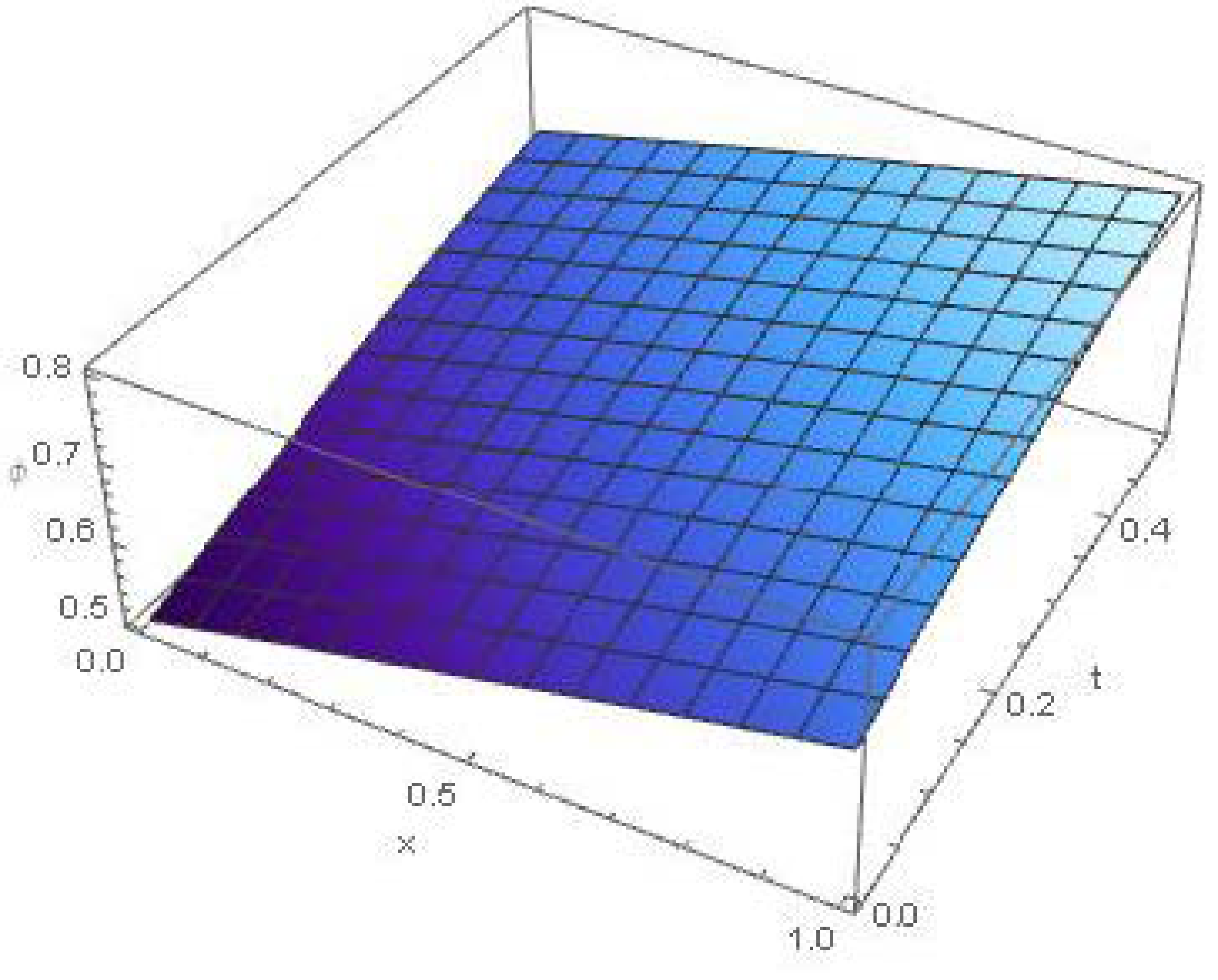
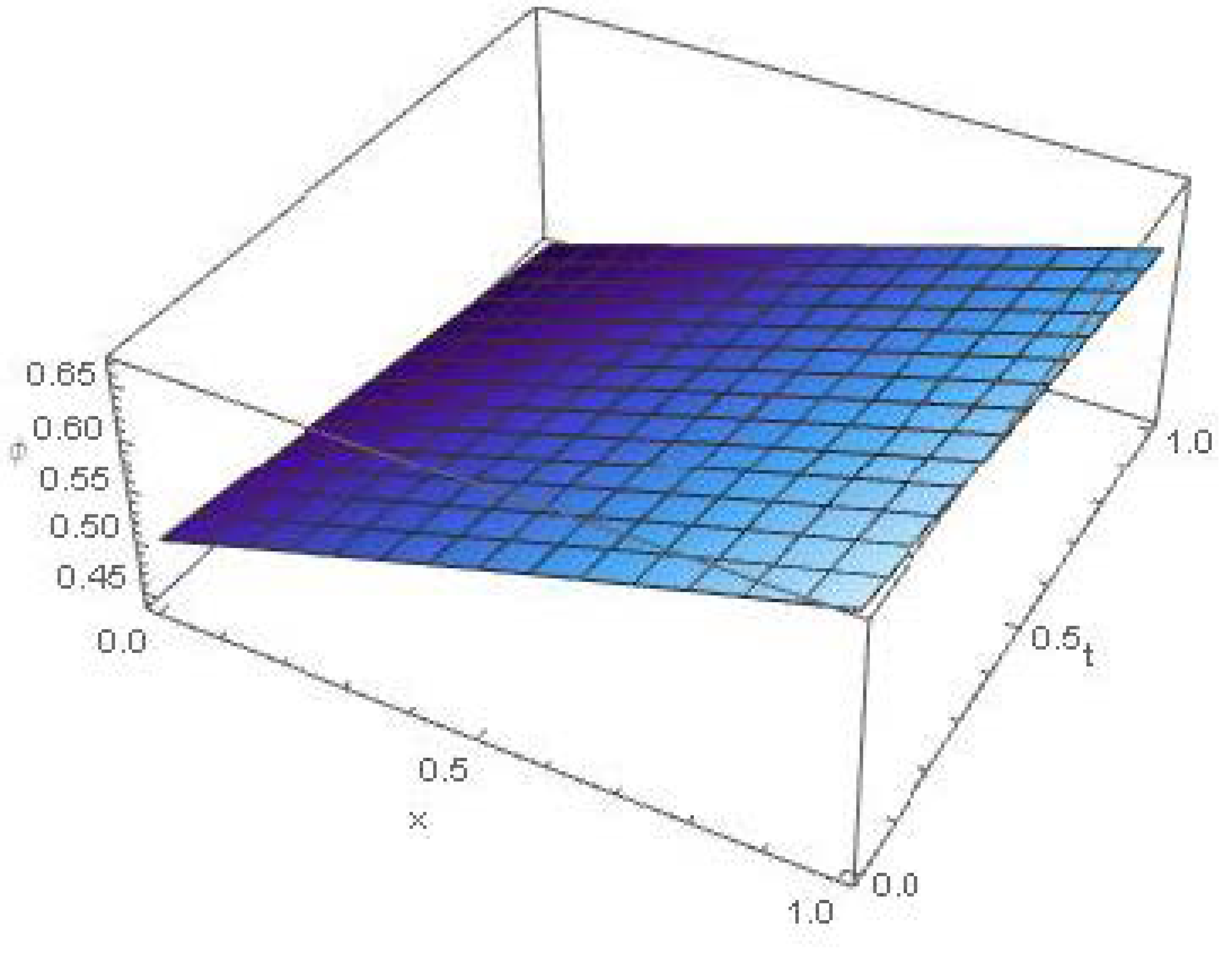
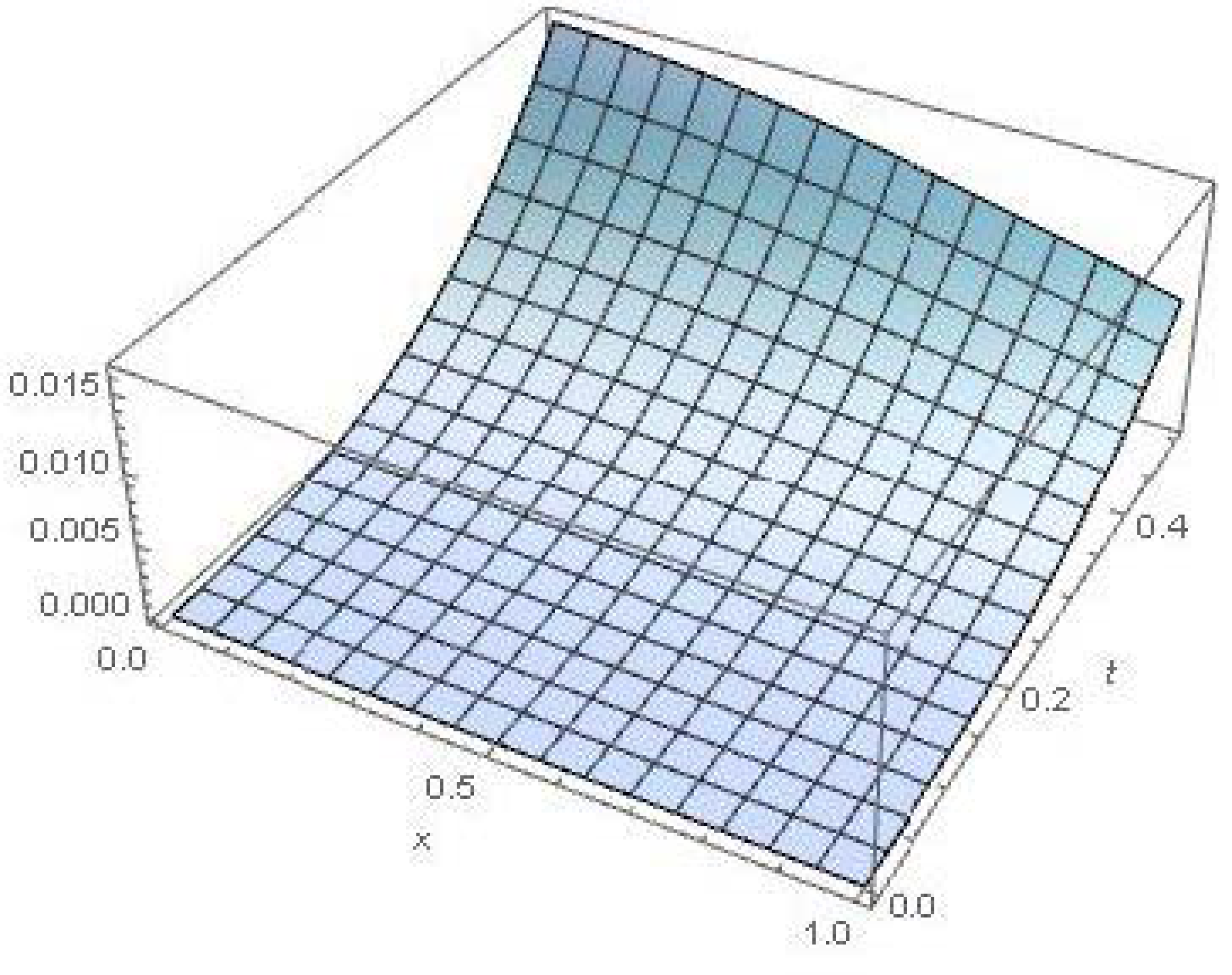
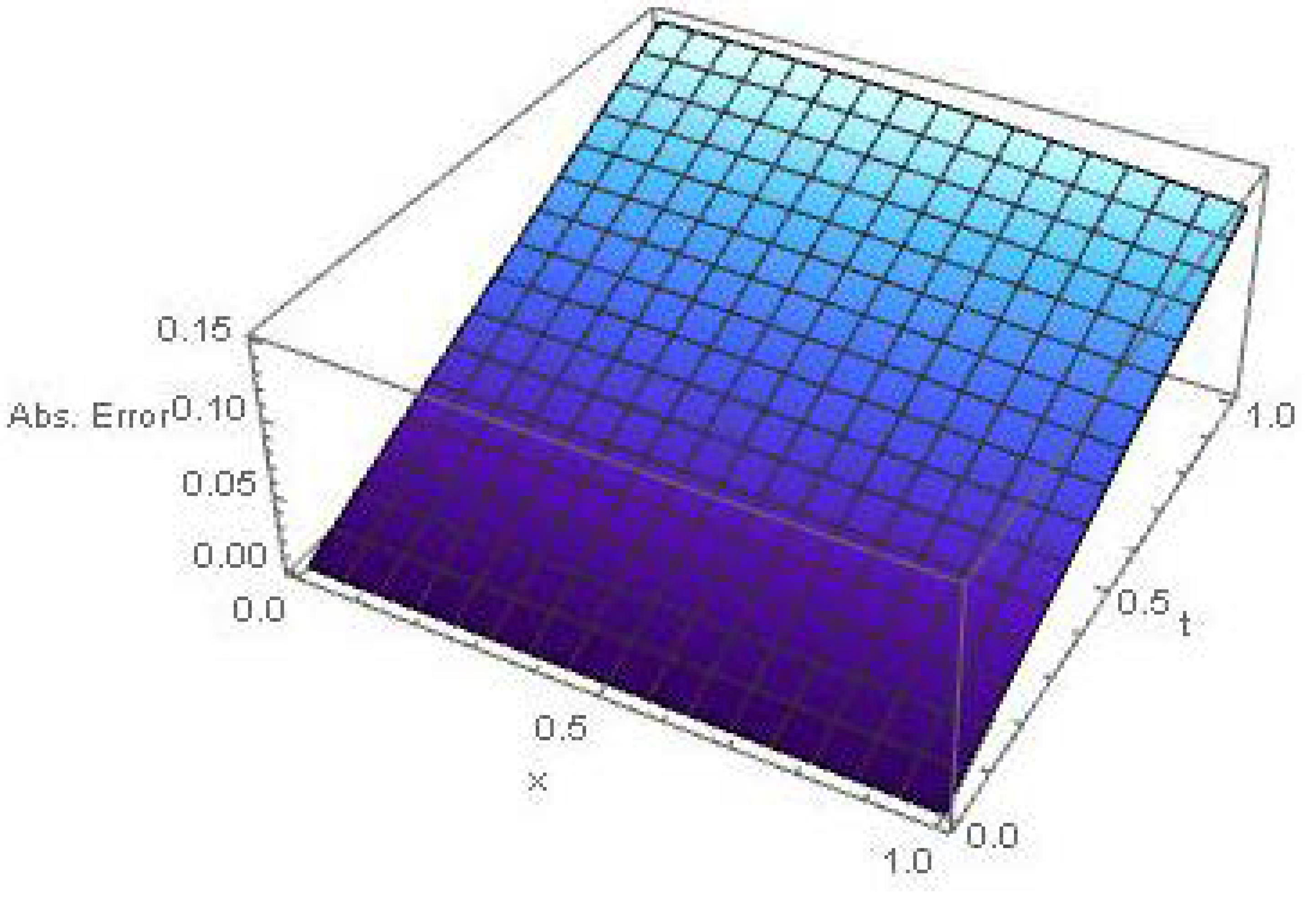
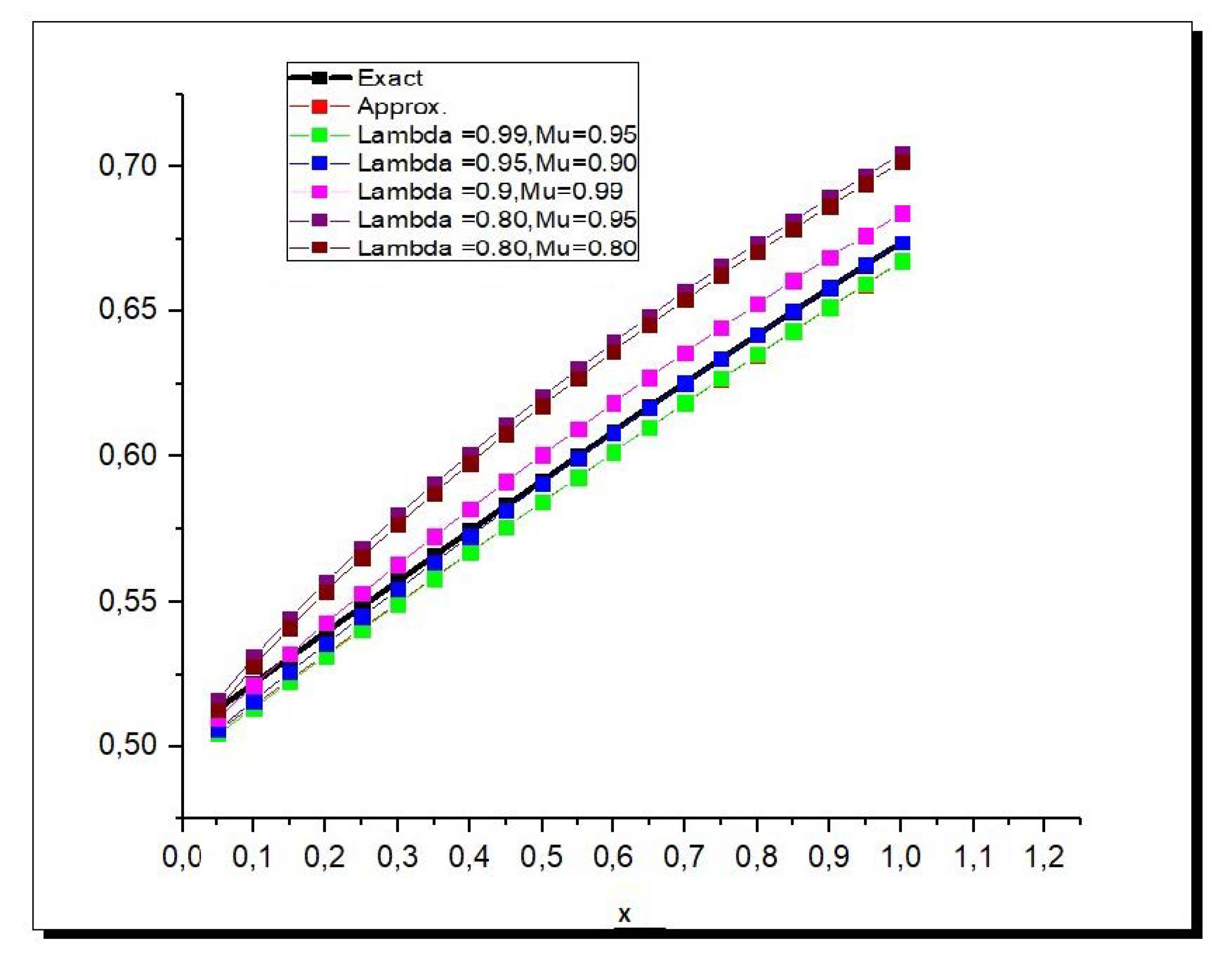
6. Results and Discussion

This segment discusses the proposed method’s precision and applicability by comparing the approximate and exact solutions using graphs and tables. Figure 1 and Figure 2, depict the behaviors of the exact solutions of Examples 3 and 4, when $\mu =\lambda =1$. We can observe that the solution $\varphi \left(\frac{x^{\lambda }}{\lambda },\frac{t^{\mu }}{\mu }\right)$ increases quickly when we increase x and t.

In Figure 3 and Figure 4 we show the behaviors of approximate solutions of Examples 3 and 4.

Figure 5 and Figure 6, the represent the absolute error between the exact and absolute solution when $\mu =\lambda =1$ and $x,t$ belong to [0,1]. These figures reveal that the approximate solutions obtained by CSDM are almost similar to the exact solutions. In both Figure 7 and Figure 8, we present various fractional-order solutions, of Examples 3 and 4, respectively, in two-dimensional space; we observe that the numerical solution becomes close to the exact solution when the fractional values $\mu ,\lambda \to 1.$

Table 1. Absolute Error for Example 3 when $\lambda =\mu =1$.

t	x	Approximate Solution	Exact Solution	Absolute Error
0.02	0.05	0.516332	0.516333	0.00000111929
	0.10	0.525155	0.525156	0.00000111497
	0.15	0.533963	0.533964	0.00000110789
	0.20	0.54275	0.542751	0.00000109809
	0.25	0.55151	0.551511	0.00000108563
0.07	0.05	0.534984	0.535031	0.0000475469
	0.10	0.543768	0.543815	0.0000473493
	0.15	0.552524	0.552571	0.0000470361
	0.20	0.561249	0.561295	0.0000466091
	0.25	0.569936	0.569982	0.0000460706
	0.30	0.57858	0.578625	0.0000454232

and

Table 2. Absolute Error for Example 4 when $\lambda =\mu =1$.

t	x	Approximate Solution	Exact Solution	Absolute Error
	0.05	0.505714	0.513255	0.00748392
	0.10	0.514549	0.522083	0.0075053
0.01	0.15	0.523374	0.530897	0.00752205
	0.20	0.532186	0.539691	0.00753415
	0.25	0.540977	0.548461	0.00754156
	0.05	0.505714	0.513255	0.00748392
	0.10	0.514549	0.522083	0.0075053
0.05	0.15	0.523374	0.530897	0.00752205
	0.20	0.532186	0.539691	0.00753415
	0.25	0.540977	0.548461	0.00754156

provide the comparison of exact and approximate solutions in term of absolute error at $\mu =\lambda =1$, at time $t=0.02,0.07$ in Example 3, and $t=0.01,0.05$ for Example 4, as x increases. In this case we can see that the solution $\varphi \left(\frac{x^{\lambda }}{\lambda },\frac{t^{\mu }}{\mu }\right)$ decreases regularly as the fractional values of $\lambda ,\mu$ increases.

7. Conclusions

This study has efficiently implemented the conformable Summdu transform and Adomian decomposition method to obtain an approximate solution of the conformable fractional Fitzhugh–Nagumo model. The CSDM gives us a solution in an infinite series with small error and high convergence. Furthermore, the convergence and the error analysis of the proposed method were stated and proven. Two examples were employed in order to illustrate the preciseness and effectiveness of the employed method. To provide better understanding of the characteristics of the solutions, the solution graphs were plotted in Figure 1, Figure 2, Figure 3, Figure 4, Figure 5, Figure 6, Figure 7 and Figure 8, by considering different values of parameters, x, and t within the interval $[0,1]$. Moreover, we have discussed the behavior of the solution $\varphi \left(\frac{x^{\lambda }}{\lambda },\frac{t^{\mu }}{\mu }\right)$ when $(\lambda =\nu =1)$ and approximate solutions when $\lambda$ and $\nu$ taking different fractional values. The obtained solutions were in full agreement as compared with exact solutions. Finally, the exact solutions and approximate solutions were plotted, and we can see the agreement among the solutions. The results lead us to say that the proposed method is reliable, accurate, and much understandable compared to other methods. Hence, it is concluded that this method can also be applied to solve other fractional non-linear differential equations involving conformable fractional derivatives.

References

1. Debnath, L. Recent applications of fractional calculus to science and engineering. Int. J. Math. Math. Sci. 2003, 54, 3413–3442. [Google Scholar] [CrossRef] [Green Version]
2. Shi, R.; Ren, J.; Wang, C. Analysis of a fractional order mathematical model for tuberculosis with optimal control. J. Nonlinear Funct Anal. 2020, 2020. [Google Scholar] [CrossRef]
3. Cernea, A. On the mild solutions of a class of second-order integro-differential inclusions. J. Nonlinear Var. Anal. 2019, 3, 247–256. [Google Scholar]
4. Kamenskii, M.; Voskovskaya, N.; Zvereva, M. On periodic oscillations of some points of a string with a nonlinear boundary condition. Appl. Set-Valued Anal. Optim. 2020, 2, 35–48. [Google Scholar]
5. Fitzhugh, R. Impulse and physiological states in models of nerve membrane. Biophys. J. 1961, 1, 445–466. [Google Scholar] [CrossRef] [Green Version]
6. Nagumo, J.S.; Arimoto, S.; Yoshizawa, S. An active pulse transmission line simulating nerve. Proc. IRE 1962, 50, 2061–2070. [Google Scholar] [CrossRef]
7. Shih, M.; Momoniat, E.; Mahomed, F.M. Approximate conditional symmetries and approximate solutions of the perturbed Fitzhugh–Nagumo equation. J. Math. Phys 2005, 46, 023503. [Google Scholar] [CrossRef]
8. Abbasbandy, S. Soliton solutions for the Fitzhugh–Nagumo equation with the homotopy analysis method. Appl. Math. Model. 2008, 32, 2706–2714. [Google Scholar] [CrossRef]
9. Li, H.; Guo, Y. New exact solutions to the Fitzhugh–Nagumo equation. Appl. Math. Comput. 2006, 180, 524–528. [Google Scholar] [CrossRef]
10. Hariharan, G.; Kannan, K. Haar wavelet method for solving FitzHugh-Nagumo equation. Int. J. Comput. Math. Sci. 2010, 2, 2. [Google Scholar]
11. Kawahara, T.; Tanaka, M. Interaction of travelling fronts: An exact solution of a nonlinear diffusion equation. Phys. Lett. A 1983, 97, 311–314. [Google Scholar] [CrossRef]
12. Nucci, M.C.; Clarkson, P.A. The nonclassical method is more general than the direct method for symmetry reductions: An example ofthe FitzhughNagumo equation. Phys. Lett. A 1992, 164, 49–56. [Google Scholar] [CrossRef]
13. Soliman, A.A. Numerical simulation of the Fitzhugh- Nagumo equations. Abstr. Appl. Anal. 2012, 2012, 762516. [Google Scholar] [CrossRef]
14. Hariharan, G.; Rajaraman, R. Two reliable wavelet methods to Fitzhugh-Nagumo (FN) and fractional FN equations. J. Math. Chem. 2013, 51, 2432–2454. [Google Scholar] [CrossRef]
15. Kumar, D.; Singh, J.; Baleanu, D. A new numerical algorithm for fractional Fitzhugh– Nagumo equation arising in transmission of nerve impulses. Nonlinear Dyn. 2018, 91, 307–317. [Google Scholar] [CrossRef]
16. Bu, W.; Tang, Y.; Wu, Y.; Yang, J. Crank–Nicolson ADI Galerkin finite element method for two-dimensional fractional FitzHugh–Nagumo monodomain model. Appl. Math. Comput. 2015, 257, 355–364. [Google Scholar] [CrossRef]
17. Pandir, Y.; Tandogan, Y. Exact Solutions of the Time-fractional Fitzhugh-Nagumo Equation. AIP Conf. Proc. 2013, 1558, 1919–1922. [Google Scholar] [CrossRef]
18. Olmos, D.; Shizgal, B.D. Pseudospectral method of solution of the Fitzhugh–Nagumo equation. Math. Comput. Simul. 2009, 79, 2258–2278. [Google Scholar] [CrossRef]
19. Ghosh, U.; Sarkar, M.; Shantanu, D. Solution of linear fractional non-homogeneous differential equations with Jumarie fractional derivative and evaluation of particular integral. Am. J. Math. Anal. 2015, 3, 54–64. [Google Scholar]
20. Wang, L.; Fu, J. Non-Noether symmetries of Hamiltonian systems with conformable fractional derivatives. Chin. Phys. B 2016, 25, 4501. [Google Scholar] [CrossRef]
21. Kareem, A. Conformable fractional derivatives and it is applications for solving fractional differential equations. IOSR J. Math. 2017, 13, 81–87. [Google Scholar] [CrossRef]
22. Adomian, G. A Review of the Decomposition Method in Applied Mathematics. J. Math. Anal. Appl. 1998, 135, 501–544. [Google Scholar] [CrossRef] [Green Version]
23. Al-Zhour, Z.; Alrawajeh, F.; Al-Mutairi, N. New Results on the Conformable Fractional Sumudu Transform: Theories and Applications. Int. J. Anal. Appl. 2019, 17, 1019–1033. [Google Scholar]
24. Abdeljawad, T. On conformable fractional calculus. J. Comput. Appl. Math. 2015, 279, 57–66. [Google Scholar] [CrossRef]
25. Atangana, A.; Baleanu, D.; Alsaedi, A. New properties of conformable derivative. Open Math. 2015, 13, 889. [Google Scholar] [CrossRef]
26. Khalil, R.; Al Horani, M.; Yousef, A.; Sababheh, M. A new definition of fractional derivative. J. Comput. Appl. Math. 2014, 264, 65–70. [Google Scholar] [CrossRef]
27. Atangana, A. Derivative with a New Parameter: Theory, Methods and Applications; Academic Press: Cambridge, MA, USA, 2015. [Google Scholar]
28. Afaqeih, S.; Bakıcıerler, G.; Mısırlı, E. Conformable Double Sumudu Transform with Applications. J. Appl. Comput. Mech. 2021, 1–9. [Google Scholar] [CrossRef]
29. Alfaqeih, S.; Misirli, E. Conformable Double Laplace Transform Method for Solving Conformable Fractional Partial Differential Equations. Comput. Methods Differ. Equ. 2021. [Google Scholar] [CrossRef]
30. Alfaqeih, S.; Misirli, E. On double Shehu transform and its properties with applications. Int. J. Anal. Appl. 2020, 18, 381–395. [Google Scholar]
31. Alfaqeih, S.; Kayijuka, I. Solving System of Conformable Fractional Differential Equations by Conformable Double Laplace Decomposition Method. J. Part. Differ. Equ. 2020, 33, 275–290. [Google Scholar]
32. El-Kalla, I. Convergence of the Adomian method applied to a class of nonlinear integral equations. Appl. Math. Lett. 2008, 21, 372–376. [Google Scholar] [CrossRef] [Green Version]
33. Eltayeb, H.; Abdalla, Y.T.; Bachar, I.; Khabir, M.H. Fractional Telegraph Equation and Its Solution by Natural Transform Decomposition Method. Symmetry 2019, 11, 334. [Google Scholar] [CrossRef] [Green Version]
Figure 1. Exact solution graph of ϕ x λ λ , t μ μ , of Example 3, when μ = λ = 1 .
Symmetry 13 00243 g001
Figure 2. Exact solution graph of ϕ x λ λ , t μ μ , of Example 4, when μ = λ = 1 .
Symmetry 13 00243 g002
Figure 3. Approximate solution graph of ϕ x λ λ , t μ μ , of Example 3, for 5th-order approximations, when μ = λ = 1 .
Symmetry 13 00243 g003
Figure 4. Approximate solution graph of ϕ x λ λ , t μ μ , of Example 4, for 5th-order approximations, when μ = λ = 1 .
Symmetry 13 00243 g004
Figure 5. Absolute error when μ = λ = 1 for Example 3.
Symmetry 13 00243 g005
Figure 6. Absolute error when μ = λ = 1 for Example 4.
Symmetry 13 00243 g006
Figure 7. Exact and approximate solutions of ϕ x λ λ , t μ μ , for Example 3, for diverse values of fractional orders μ , and λ when t = 2 100 .
Symmetry 13 00243 g007
Figure 8. Exact and approximate solutions of ϕ x λ λ , t μ μ , for Example 4, for diverse values of fractional orders μ , and λ when t = 5 100 .
Symmetry 13 00243 g008