Abstract
We discuss quantum time states formed with a finite number of energy eigenstates with the purpose of obtaining a time coordinate. These time states are eigenstates of the recently introduced discrete time operator. The coordinate and momentum representations of these time eigenstates resemble classical time curves and become classical at high energies. To illustrate this behavior, we consider the simple example of the particle-in-a-box model. We can follow the quantum-classical transition of the system. Among the many existing solutions for the particle in a box, we use a set which leads to time eigenstates for use as a coordinate system.
1. Introduction
The subject of time in quantum mechanics is an old subject of interest. The oldest way to deal with time in quantum mechanics is the quantization of the classical expression for the time of a classical free particle, , where X is the observation point [1]. In this approach, there are the problems of the ordering of operators and the divergence at the momentum . The time evolution of the eigenstate of the resulting operator, a plane wave in momentum space times a scaling factor, was the time state. Since the spectrum for the free particle is continuous, there is no conflict with the Pauli theorem which rejects the existence of a time operator when the spectrum of the Hamiltonian is discrete [2]. The properties of those time operator and states were further developed by several authors, some against the existence of a time operator and others finding them and their properties. Some of these authors are: Kijowski, Giannitrapani, Allcock, Baute, Egusquiza, Muga, Sala, Beauregard, Bokes, Busch, Delgado, Egusquiza, Damborenea, Galapon, Hall, Holevo, Isidro, Kobe, Razavy, Leavens, Ol’khovskii, and many others [3,4,5]. Other interesting developments were made by Arai, who stated the properties of time operator [6] among other properties of time operators for discrete energy spectrum [7].
For the discrete spectrum case, Weyl quantized the momentum operator on the circle, with an equidistant spectrum [8]. The eigenfunctions were the roots of the unity and the momentum operator needed of values at all points of the mesh. A development of this was done by Santanam also for an equidistant spectrum getting a momentum operator which also needs of values at all the points of a finite mesh. Afterwards, Galapon considered a square absolutely convergent sequence using the full infinite discrete spectrum resulting in an expression similar to that used by Weyl, but with different factors. It needs of the differences between all the points of the spectrum. On the other hand, there is the common belief that a time operator is related to the derivative with respect to the energy. Thus, we need a way of doing that when the spectrum of the Hamiltonian is discrete, and may be not equidistant. Additional properties of discrete momentum operators were developed by Santhanam [9].
We use a non-standard finite differences derivative [10,11,12,13,14,15,16,17,18,19,20,21] to define a quantum time operator as the discrete derivative with respect to the energy, and then find quantum densities which can be called a “quantum time axis” for quantum systems with discrete spectrum. The time state we use in this paper is similar to the non-normalizable eigenstate of a canonical momentum of a label operator, with an equidistant spectrum, used and developed by Cannata [22]. However, the time eigenstates we construct are formed with a finite number of energy eigenstates. The time axis can be obtained with few energy eigenstates. An advantage of using a finite number of energy eigenstates is that the resulting time state can be normalized, and then, it belongs to the Hilbert space.
We use here a non-standard discrete derivative with the characteristic that it has the complex exponential function as its eigenvector [10]; a property which can be used to define a time operator which complies with discrete versions of the properties that the continuous variable operator has [23]: symmetry, self-adjointness, deficiency indices, self-adjoint extensions.
Our point of view is that the time eigenstates are a coordinate axis for quantum systems, in the same way as the usual coordinate eigenstates are a coordinate axis in terms of which a representation of the abstract kets and operators can be written. We discuss the coordinate and momentum representations of these partial-time eigenstates and how they can be used to define coordinate and momentum time densities. These densities are concentrated around the classical trajectory. The partial time eigenstates change their behavior with the range of energies of the involved energy eigenstates. At low energies, the coordinate and momentum densities show the full quantum behavior. At higher energies, the time eigenstates follow better the classical trajectory.
In Section 2, we briefly review the discrete derivative that we use and some of its properties, adapted to be a discrete derivative with respect to a discrete energy spectrum of some quantum Hamiltonian.
The time operator based on a discrete derivative can also have the properties that the continuous variable operator has, but in a discrete form. In Section 3 it is shown that the discrete time operator can be symmetric, in a discrete way, which is a requirement for an operator to be an observable.
The definition and properties of time eigenstates, formed with the full set of energy eigenstates, is the subject of Section 4, whereas the time states formed with a finite set of energy eigenstates is discussed in Section 5.
To illustrate the use of these concepts, we apply our scheme to a simple model. We consider the partial-time eigenstates for the particle in a box in Section 6. The particle in a box is still a subject of interest [24,25,26,27]. We find that the coordinate and momentum representations of the time eigenstates are concentrated around the classical or curves. Among the many existing sets of solutions for the particle in a box, we use truncated plane waves. These functions are simultaneous eigenfunctions of the momentum and of the kinetic energy operators, and give rise to time eigenstates which can be used as a coordinate system.
At the end of the paper there are some concluding remarks.
2. A Discrete Derivative
We briefly review the discrete derivative that we will use in what follows [10]. The discussion is oriented towards performing discrete derivatives with respect to the energy spectrum of a given quantum Hamiltonian with pure point spectrum.
Consider a quantum system with Hamiltonian which has the pure point spectrum . The Hamiltonian is not time-dependent, and each energy level can be degenerate with degeneracy index . The set of energy eigenvectors is denoted by . An unspecified j and energy eigenket is denoted by just . The working space is the complex Hilbert space H defined as
for which is an orthonormal basis, with the usual inner product .
We will consider the subspace spanned by the eigenstates with eigenenergies from to , , . This finite number of energy eigenvalues is seen as a partition of the bounded interval , with spacing between points denoted by .
For each partition , the following discrete derivative operators, with respect to the energy spectrum, are defined
where backward and forward derivatives are defined as
and the denominators in these operators are defined as
The ± signs (for forward and backward time evolution) are the signs of the exponential functions . These functions are the exact eigenfunctions of the discrete derivatives
where
regardless of the values of t and of the ’s. The derivative has other eigenfunctions with real eigenvalues, but they describe decaying states or a source, and a discrete derivative with those functions as eigenfunctions requires of other denominators. Those states require of another paper devoted just to them.
Please note that the discrete derivative operators (2a) and (2b) can act on the entire Hilbert space spanned by . However, since they depend on the partition their effect will be different from zero only on that partition . They are also of finite dimensional range, hence, we can represent them by finite dimensional matrices, if needed.
As indicated in the limits of the above sums, we should be careful not to include differences between non-existing states. For the sake of notation, we will omit to write the upper limit of sums over , with the understanding that such sums are over the allowed degeneracies.
For the arbitrary ket , , the components of its derivatives are
They define how the derivatives are acting on ket components , or on functions evaluated at the mesh points, as a backward or forward derivative. In case there is no degeneracy, the index should be dropped from all these equalities.
We can recover the usual finite differences derivative from Equations (8a) and (8b), if needed, when and are approximated to zeroth order in t and first order in ’s, because
However, in this paper, we need any value of t and the ’s must be finite and fixed because they will be the differences between the energy eigenvalues of a Hamiltonian with pure point spectrum. Thus, we will not take the limit at all.
Since these discrete derivative operators can be represented by square matrices, from Equation (5) it follows that the variable is itself a parametric eigenvalue of the matrices, with corresponding eigenvector whose entries are the complex exponentials . The matrix form will give rise to other eigenvectors, but they are not useful for our purposes.
3. A Discrete Symmetric Operator
The adjoints of the discrete derivatives operators (3a) and (3b), times the imaginary unit i, are
where the symbol † indicates the adjoint of the operator. The summation of these equalities leads to the relationships
These equalities are rewritten as
where
and
are the backward and forward versions of a time-like operator. We argue that both backward and forward operators and are just different versions of the same thing and we will use them based on this idea.
Definition 1.
The discrete operators and are said to be a symmetric pair of operators if the relations
hold on the domain , where
Since the space on which these time operators act –the set , , —is the same, we can say that they are a self-adjoint pair of operators.
Wave functions such that const., for all , belong to the domain of the time operator. This is the property of the time eigenstates that we will introduce below, constituting a part of the domain of the time operator.
The quantities (13) can be seen either as the change of the energy density with respect to the energy, or they can be separated into boundary and “unharmonicity” terms inside the interval , as we explain next.
The rewriting of the quantities and provides for another interpretation of them because they can be split into boundary and a remaining term,
where
Usually, the coefficients in these sums become smaller and smaller as j increases. Thus, by choosing larger than ten, let us say, the values of and will be very small.
Then, a solution of the vanishing boundary condition, , evaluated between and , can be given as follows
or
On the other hand, the anharmonicity terms
evaluated between and , vanish when the energy values are equidistant, i.e., when the ’s are equal. Thus, the equidistant spectrum case is also part of the domain of the time operator, as long as the boundary conditions, , are fulfilled.
For other systems with non-equidistant energy spectrum, will be very small with a small number of oscillations in it and it will diverge when the denominator evaluates to zero, at the Bohr’s times and at its multiples. Recall the relationship , i.e., both have the same zeroes and hence both define the same singularities because they appear in the denominators of (20a) and (20b).
The domain of the time operator also contains vectors such that a part of the sum (20a) and (20b) cancels the remaining of it.
If we evaluate the unharmonicity term (13) with the same vector, we get
which is the derivative of the energy probability density, when the system is in the state , with respect to the energy. Therefore, a change of this sum indicates that the composition of the wave function, in terms of the energy eigenstates, has changed.
4. Time-Dependent States
The states we work with are formed with the energy eigenstates such that their Fourier coefficients are supported in .
Consider the usual time-dependent ket,
The magnitude of the coefficients decrease with increasing k for the state to be normalizable, . We can think of the coefficients of the time-dependent state (22) as being the projection of the state on the time-dependent vectors , a complete set of vectors in the Hilbert space.
Definition 2.
The time ket is defined as
where .
The time state is a generalized ket because it is not normalizable and then it does not belong to the Hilbert space, but it can be used as an axis in the same way as the eigenfunctions of the momentum operator are not normalizable but are used to give a representation to an abstract ket. In next section, we overcome this problem by using just a finite number of terms to form a partial-time ket.
Similar time states were used by several authors before [28,29]. These states evolve backwards in time.
Let us analyze the behavior of the inner product between time states. Consider the N-th partial sum
where is the projector on the first N energy eigenstates. When the spectrum is equidistant (the harmonic oscillator), , and with the same degeneracy g for all energy levels, we get
The value of this quantity reaches its maximum modulus when , thus
and this time, the Bohr time , is also its period. Thus, the function gets closer to a set of scaled Kronecker delta functions centered at , . At other points, the function oscillates with small values and it becomes zero at and at its multiples. Thus, the zeroes become closer and closer from each other as N increases. The function is similar to the Dirichlet kernel. For instance, for the quantum oscillator, its energies are given by , There is a global phase , and then, we consider the squared modulus of
Its period is .
Considering a finite arbitrary subset of energy eigenvalues such as , in general the function will not be a periodic function, but it will be a trigonometric polynomial. This type of functions is a generalization of the periodic functions called the almost periodic functions [30], a particular case of which are the trigonometric polynomials [31]. Accordingly, the quantity belong to the almost periodic functions. Recall that a trigonometric polynomial is a finite complex linear combination of elements of the set .
An almost periodic function complies such that, for each , there exist an such that, in each interval , there is at least one such that
The collection of such is called -almost periods of f. In general, it is difficult to find these almost periods of an almost periodic function.
Even more, the Bohr’s property (28) is taken beyond of complex valued functions, namely to functions , with an arbitrary complex or real Banach space [31]. In particular, we can take the Hilbert space we work with. f is called almost periodic if it basically satisfies the previous definition but by replacing the complex modulus by the corresponding norm in (28). An immediate example of such almost periodic functions is, in fact, the states we are considering (22), they are trigonometric polynomials with coefficients belonging to the corresponding Hilbert space such that (28) is left as
where we have assumed to be normalized, and where ℜ stands for the real part of its argument.
The space for the time states (considering the time variable) is the Besicovitch space. In the Appendix A, we show that the time states are indeed orthogonal in that space, and therefore they are a basis for the time-dependent kets.
The time derivative of the time ket is
which is just the (backward evolution) Schrödinger equation of motion. Please note that the zeroes due to the denominators are not present in Equation (30). Furthermore, this time ket satisfies the conjugate of the Schrödinger equation of motion
where is the j-th component of the ket . These equations are similar to (5) but written in ket form, thus, there are no singularities in they neither.
5. Partial-Time Eigenstates
The time ket (23) is not normalizable and then it does not belong to the Hilbert space, but any time-dependent ket is written in terms of it. However, a finite sum will lead to states which belong to the Hilbert space. If the coefficients in Equation (22) are different from zero for a subset of energies from to , let us say, then we can use only the corresponding part of the time ket. We will study these states for a simple example model below just to understand the behavior of such states.
Definition 3.
The partial-time state is
where , and , .
The partial-time states are normalized eigenstates of the time operator, with eigenvalue t, and can be used as part of a coordinate axis because they contain the energy eigenstates with the same weight. We now ask for the times for which the partial-time states can be orthonormal.
The inner product between partial-time eigenstates is
When the spectrum is equidistant, , and with the same degeneracy g for all levels, we get
The value of this function when , , is . Its period is also . At other points, the function oscillates with small values and it becomes zero at and at its multiples. Thus, the zeroes become closer and closer from each other as the difference increases.
We next illustrate what the partial-time states are by considering a simple system, just to fix ideas.
6. Application. The Particle in a Box
The energy eigenvalues for the particle in the infinite well potential
are , . The associated wave function space is known to be . We consider the normalized truncated plane waves
which form an orthonormal basis for . Here is the characteristic function of the interval . Let us recall that aside from the fact that these functions do not vanish at the boundaries , they form a set of eigenvectors common to the momentum and the kinetic energy operators (for this quantum system) in the common sense: they satisfy the corresponding eigenvalue equations and belong to the domains which provide the self-adjointness to such operators [23]. This fact allows us to associate two momentum eigenvalues, , to each energy eigenvalue, through the relationship . Consequently, the degree of degeneracy for each energy level is two.
The energy differences for this system are not equally spaced but . This gives rise to the well-defined characteristic times for the system. We can identify them as the times spent by the quantum particle when going from one of the walls to the other wall. The momentum changes sign when the particle hits the wall. This is a sudden change in the composition of the wave function and, at those instants of time, the time operator no longer is discrete symmetric.
We use the normalized partial-time eigenstate
formed with momentum and energy eigenstates.
To illustrate the behavior of , in Figure 1, we have plotted the quantity , which depends only on the difference , with 100 terms, from to , and for the infinite well potential. It is a function that approximates a delta function with noise. Please note that there are larger oscillations starting around the time that a classical particle with energy spends going from one wall to the other, or the Bohr time (these times are similar). We have observed this behavior for any number of states N, becoming narrower and narrower and taller and taller as N increases. Therefore, as N increases, this function approaches better a delta function with a small number of oscillations added to it; we call this property the discrete orthogonality of time states. However, these functions are orthogonal indeed in the Besicovitch space, as is shown in the Appendix A. The Besicovitch space is the space to consider when dealing with almost periodic functions, which is the case of the time states.
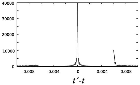
Figure 1.
A plot of , with 100 terms, from to , and for the infinite well. This function depends only on the difference . The arrow indicates an increase on the height of oscillations and correspond to the time that a classical particle with energy spends when going from one wall to the other, a change in the evolution of the system. This function is periodic. Dimensionless units.
The function is periodic, with the same period regardless of how many terms are considered, when the sum goes from one to . To see this, we substitute the energies into Equation (24), finding that the function
has the period as can be easily verified.
The time states are orthogonal, and the partial-time states are a part of them. But the partial-time states are also orthogonal sometimes (the zeroes of ). In Figure 2 we have plotted the values of and of , with fixed, for which is zero. In the figure, there are the cases and and several values of . At low energies and few terms in there are fewer values of for which the time states are orthogonal. The set of values gets denser when the energy is larger.
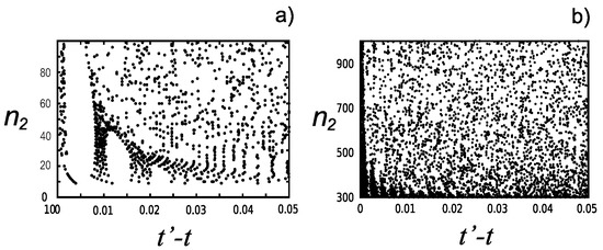
Figure 2.
Zeroes of for partial-time states formed with (a) states with and from to and (b) states with and from to , for the particle in a box. The vertical axis indicates up to which state is included in . The partial states can also be orthogonal for some particular times and values of and . Dimensionless units.
A quick calculation shows how classical dynamics is behind quantum motion. Let us take only the two states with energies and with positive momentum only, then, the squared modulus of the partial-time state, in the coordinate representation, is
a function which is a wave moving accordingly to a classical particle moving with momentum . In particular, if this momentum is . Then, a classical analogue of a quantum partial-time state can be a set of particles with these momentum values. Let us recall that the discrete time operator takes adjacent energy levels to compute the discrete derivative.
Now, the distance that a classical particle travels in a Bohr time with momentum is
which is the width of the well. Hence, the Bohr times correspond to the times that a particle with momentum spend when going from one wall to the other.
Actually, there are three options for defining partial-time eigenstates. We can use only negative, , or only positive, , momentum energy eigenstates, or we can use both states in Equation (37), depending on our interest.
To illustrate what the partial-time states look like, we have made several calculations with different energy eigenstates.
If we include negative and positive momentum states, with and , we have that the coordinate representation of the partial-time state is
Then, at we get
Hence, the coordinate representation of the time state is the time evolution of a scaled delta function centered at the origin. For a finite range of values of and we will be dealing with a function less narrow than a delta function.
The function is also periodic in time with period : . This is evident when we write as
At half the period, when , there is a change in the composition of the time state. By evaluating at , we find that
Thus, half the state is now located around and the other half is located at the right wall, at . At that instant of time, the part that was moving towards the left is replaced by a function that moves towards the right and vice versa.
When only positive momentum energy eigenstates are used, in Figure 3 there is a three-dimensional plot of the corresponding density . We have considered partial-time states formed with the states one and two, with the states one to six and one to the 12-th positive momentum energy eigenstates. These densities tend to be concentrated around only the positive momentum part of classical trajectories departing from the origin of coordinates and moving backwards in time with momentum . The density spreads quickly as it evolves in time, and there is some oscillations in them. These partial-time states are useful if one is interested on motion only to the right or only to the left. The mirror image around the origin of coordinates gives the negative momentum density.
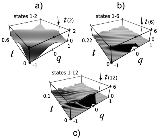
Figure 3.
Three-dimensional plots of the coordinate density for the infinite well. These states were formed with little low energy, positive momentum, energy eigenstates. Partial-time states formed with energy eigenstates (a) from one to two, (b) from one to six, and (c) from one to the 12-th energy eigenstate. Dimensionless units.
At this stage, we will content ourselves by giving a general characterization of the (almost) oscillatory behavior for the density . First, note that we can consider as a trigonometric polynomial, in t, and depending on the parameter q. For each fixed q, the coordinate representations are seen as coefficients spanned by the set . Thus, realizing that the product of two trigonometric polynomials is also a trigonometric polynomial, it follows that and will have the Bohr’s property (28) at each value q. It is another advantage of considering with a finite number of energy eigenstates; the Bohr’s property is a general feature of the density constructed with the energy eigenstates. Similarly, the momentum density is an almost periodic function.
By looking at the place in which the density is higher, we identify the arrival of the density at one of the walls; it happens, approximately, at half the Bohr times or at the time that a classical particle with the quantum momentum spends traveling from the origin to the wall. These times are indicated with an arrow in Figure 3 [32,33]. The density starts to move from the origin, , towards the left wall, . As we increase the number of states that form the time substate, the more defined the path of the particle is, with some oscillations added to it. This characteristic is similar to approximating a function by adding waves with different frequencies, as is done with the Fourier series of a function. In the figure, we can also see the positive momentum part of the evolution of partial-time state with negative momentum, a density which starts to move from the origin towards the right wall.
Now, a three-dimensional plot of the squared magnitude of the momentum representation of the partial-time states, , is shown in Figure 4. We recognize a bit of the classical behavior of particles in a box. The density is different from zero for negative momentum values, with a noticeable change in behavior at the time that the particle hits the wall (indicated with an arrow). This calculation shows that we used only positive momentum energy eigenstates to form the partial-time state.
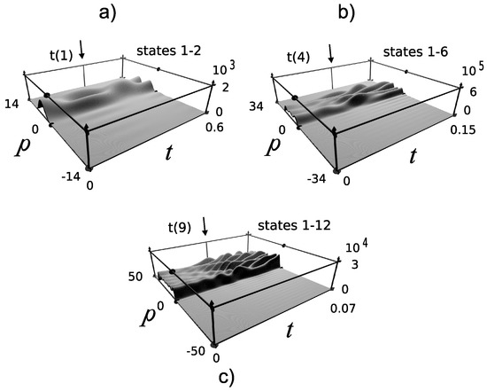
Figure 4.
Three-dimensional plots of the momentum density for the infinite well. These states were formed with few, positive momentum, low energy eigenstates. We are using (a) states one and two, (b) from states one to six, and (c) from one to the 12-th energy eigenstates. Dimensionless units.
In Figure 5 we make another set of calculations of in which we take ten or 50 energy eigenstates around some energy values, incorporating both negative and positive momentum energy eigenstates. The use of 50 states is enough to get a well-defined density around the classical path, better defined when the energy is large. There are large peaks due to the interference between positive and negative momentum parts of the density. This interference was not present when only positive momentum energy eigenstates were used, and it appears because the part of the density which is arriving on the wall interfere with the part that is leaving the wall.
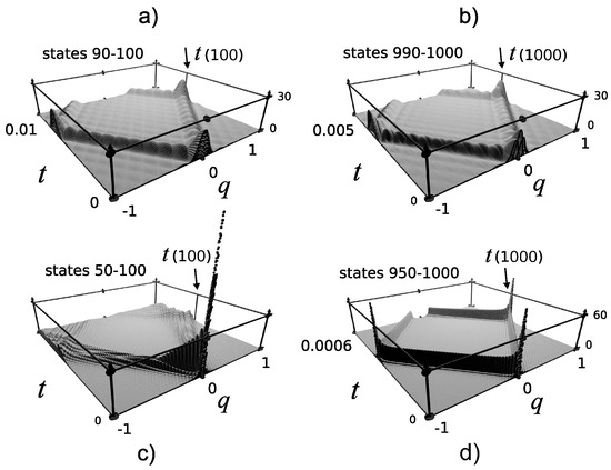
Figure 5.
Three-dimensional plots of the coordinate density for the infinite well, with only 10 or 50, negative and positive momentum, energy eigenstates. The density resembles the classical behavior at large energies. At low energies, oscillations dominate the evolution of the density. Time states formed with (a) states 90 to 100, with states (b) 990 to 1000, (c) 50–100, and (d) 950–1000. Dimensionless units.
For small values of energy there is a large number of oscillations going on which dominate the density, becoming less for larger energies. The corresponding momentum densities are shown in Figure 6. The density behaves more classically for large energies, concentrating around the classical momentum, , of a particle in a well.
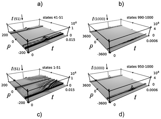
Figure 6.
Three-dimensional plots of the momentum density , in the momentum space, for the infinite well using ten or 50, negative and positive momentum, energy eigenstates. Even with the use of only ten states we get a density which resembles the classical behavior at large energies. At low energies, oscillations dominate the evolution of the density. Time states formed with (a) states 41 to 51, with states (b) 990 to 1000, (c) 1–51, and (d) 950–1000. Dimensionless units.
Even though averages give only a rough idea of the behavior of the system, there are plots of the average of the coordinate and of the coordinate width of the partial-time state in Figure 7. In the upper row of that figure we have used only two energy eigenstates to form the partial-time state. The average of the coordinate oscillates, similarly to the time evolution of the coordinate of a classical particle, and the coordinate width also oscillates but many times is small. In the lower row the calculation was made with 200 energy eigenstates causing that the shape of the state to hold for less time and get dispersed compared with the few-energy-states case. The partial-time state is well defined initially (the width is small most of the time), but it ends up dispersed. Recall that this system is periodic in time, so after the period, the initial state is recovered.
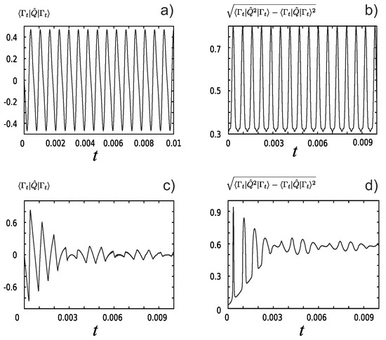
Figure 7.
Averages and widths for the partial-time state and for the particle in a box, with different amounts of energy eigenstates. Average of the coordinate with (a) states from 998 to 1000, (c) states from 800 to 1000, and coordinate width with (b) states from 998 to 100, and (d) from state 800 to 1000. Dimensionless units.
These densities can be interpreted as the partial-time states in the coordinate representation, or as the time dependence of the quantum coordinate; the quantum analogue of a density concentrated around a classical path , and similarly for the momentum densities.
Actually, our scheme can be seen as the quantum analogue of the classical method to define a time coordinate variable, a construction which allows definition of a time dynamical variable, assigning a time value to a point in phase-space, as is shown in Figure 8. In that calculation, we take the line , as the initial time curve and propagate it in time. The generated set of curves are the time curves, curves for which the time variable is a constant and contain all energy values of interest [34].
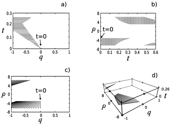
Figure 8.
A classical time surface for the particle in the box. the curve , is taken as the zero time curve and its time evolution generates the time surface. This procedure assigns a value of time to each point in phase-space. Classical partial-time states in (a) space, in (b) space, in (c) phase-space, and (d) in space. The support of the squared modulus of the quantum partial-time states resemble (a,b) in coordinate and momentum representations, respectively. Dimensionless units.
We can compare these results with the ones obtained by means of the quantization of the classical time of a free particle. The corresponding time state is concentrated at the initial point, but it spreads on the whole real axis as soon as the time increases. In our case, the densities follow the classical path.
7. Conclusions
We have shown that the use of a non-standard discrete derivative, and of time eigenstates, leads to the definition of a quantum time axis and to new insights on the relationship between quantum and classical motion, as was demonstrated for the particle in the infinite well potential.
We have also seen that time quantum densities transform into time classical densities when they contain a finite number of energy eigenstates and when the energy increases. Quantum oscillations dominate the dynamics at low energies causing that the classical dynamics be a bit difficult to recognize but the classical dynamics still dominates the quantum motion.
Time estates, with an infinite number of energy eigenstates, are not square summable. But a partial-time state is a part of the time state and it is normalizable, it contains a finite number of energy eigenstates and can be used when the system moves in that range of energies.
We have found quantum densities for single, or few, particles evolution. This is different from the quantum trajectories found with the help of equations such as the master equations of motion which describes an ensemble of particles, and also different from quantum jumps theory [35,36,37,38,39].
The time states we have introduced here are well suited to be a coordinate axis for quantum systems because time is a constant and they contain all the energy states of interest.
The goal is to define an energy-time coordinate system that will allow us to pass from a parametric description of quantum dynamics, in terms of coordinate or momentum representations, to a non-parametric representation in which time and energy are the independent variables.
With the choice of energy eigenfunctions made in this paper we obtained a time variable which can be used as part of a coordinate system, but other solutions used for the particle in a box provide with other useful quantities, the subject of a forthcoming paper.
There are many good works regarding time and Hamiltonian operators, such as the results of Arai [6,7]. However, they seem to be developed having in mind that the independent variable is continuous, as is evident in the definition of a symmetric operator. With this paper, we are introducing the concepts used in usual operator theory to the discrete realm. The continuous variable results should be taken to the discrete variable space, but these results will be a bit different.
Finally, it is not possible to take the continuous limit of the objects introduced in this paper because the energy values are fixed. But the continuous spectrum case can be found in Ref. [40].
Author Contributions
All authors have contributed equally. All authors have read and agreed to the published version of the manuscript.
Funding
This research received no external funding.
Institutional Review Board Statement
Not applicable.
Informed Consent Statement
Not applicable.
Data Availability Statement
Not applicable.
Conflicts of Interest
The authors declare no conflict of interest.
Appendix A
We now show another way to see that the partial-time kets form a basis, in the sense of Dirac. We need to show the closure and the orthonormality relations of these generalized kets. The space of this basis project is indeed a closed subspace of the Besicovitch space [29], but we will not go further in this topic because our approach focus on the partial-time eigenkets.
For the sake of simplicity, let us suppose that there is no energy degeneracy. Let and denote the partial-time eigenstate formed with the first N energy eigenstates and the time eigenstate with the full set of them, respectively. We recognize the projection of each state on the time state,
to be an almost periodic function in the sense of Besicovitch. Indeed, since and the energy spectrum is countable, is said to be a -function. By virtue of the Bohr’s fundamental theorem extended to the -functions, the norm of the state can be computed from as follows
It is called the mean value of the function . Similarly, the mean value of yields the representation of the inner product . On the other hand, we have
This equality is justified because the mean value
exists and is well defined for the almost periodic functions in the sense of Besicovitch. Even more, this quantity is different from zero at the energy levels such that .
From Equation (A2) we see that their closure relation takes the form
As regarding the orthonormalization of the time eigenkets, from Equation (A3) we can see that converges to a Dirac such as distribution respect to the Besicovitch measure, analogous to how the test functions converge in the sense of a distribution to the periodization of the Dirac function for periodic functions, respect to the Lebesgue measure.
References
- Aharonov, Y.; Bohm, D. Time in quantum theory and the uncertainty relation for time and energy. Phys. Rev. 1961, 122, 1649. [Google Scholar] [CrossRef]
- Pauli, W. Handbuch der Physik; Springer-Verlag: Berlin, Germany, 1926; Volume 23. [Google Scholar]
- Muga, J.G.; Mayato, R.S.; Egusquiza, I. (Eds.) Time in Quantum Mechanics, 2nd ed.; Lecture Notes in Physics 734; Springer: Berlin, Germany, 2008; Volume 1. [Google Scholar]
- Muga, J.G.; Mayato, R.S.; Egusquiza, I. (Eds.) Time in Quantum Mechanics; Lecture Notes in Physics Monograph 72; Springer: Berlin, Germany, 2008. [Google Scholar]
- Muga, J.G.; Ruschhaupt, A.; del Campo, A. (Eds.) Time in Quantum Mechanics; Lecture Notes in Physics 789; Springer: Berlin, Germany, 2009; Volume 2. [Google Scholar]
- Arai, A. Spectrum of time operators. Lett. Math. Phys. 2007, 80, 211–221. [Google Scholar] [CrossRef]
- Arai, A. Necessary and sufficient conditions fir a Hamiltonian with discrete eigenvalues to have time operators. Lett. Math. Phys. 2009, 87, 67–80. [Google Scholar] [CrossRef]
- Weyl, H. The Theory of Groups and Quantum Mechanics, 2nd ed.; Dover Publications, Inc.: New York, NY, USA, 1950. [Google Scholar]
- Santhanam, T.S.; Tekumalla, A.R. Quantum mechanics in finite dimensions. Found. Phys. 1976, 6, 583–587. [Google Scholar] [CrossRef]
- Martínez-Pérez, A.; Torres-Vega, G. Exact finite differences. The derivative on non uniformly spaced partitions. Symmetry 2017, 9, 217. [Google Scholar] [CrossRef]
- Mickens, R.E. Nonstandard Finite Difference Models of Differential Equations; World Scientific: Singapore, 1994. [Google Scholar]
- Mickens, R.E. Discretizations of nonlinear differential equations using explicit nonstandard methods. J. Comput. Appl. Math. 1999, 110, 181–185. [Google Scholar] [CrossRef]
- Mickens, R.E. Nonstandard Finite Difference Schemes for Differential Equations. J. Differ. Equ. Appl. 2010, 8, 823–847. [Google Scholar] [CrossRef]
- Mickens, R.E. (Ed.) Applications of Nonstandard Finite Difference Schemes; World Scientific: Singapore, 2000. [Google Scholar]
- Mickens, R.E. (Ed.) Advances in the Applications of Nonstandard Finite Difference Schemes; World Scientific: Singapore, 2005. [Google Scholar]
- Mickens, R.E. Calculation of denominator functions for nonstandard finite difference schemes for differential equations satisfying a positivity condition. Numer. Methods Partial Diff. Equ. 2006, 23, 672–691. [Google Scholar] [CrossRef]
- Tarasov, V.E. Exact discretization by Fourier transforms. Commun. Nonlinear Sci. Numer. Simul. 2016, 37, 31–61. [Google Scholar] [CrossRef]
- Tarasov, V.E. Exact Discrete Analogs of Derivatives of Integer Orders: Differences as Infinite Series. J. Math. 2015, 2015, 134842. [Google Scholar] [CrossRef]
- Tarasov, V.E. Exact discretization of Schrödinger equation. Phys. Lett. A 2016, 380, 68–75. [Google Scholar] [CrossRef]
- Potts, R.B. Differential and Difference Equations. Am. Math. Mon. 1982, 89, 402–407. [Google Scholar] [CrossRef]
- Potts, R.B. Ordinary and partial differences equations. Austral. Math. Soc. Ser. B 1986, 27, 488–501. [Google Scholar] [CrossRef]
- Cannata, F.; Ferrari, L. Canonical conjugate momentum of discrete label operators in quantum mechanics I: Formalis. Found. Phys. Lett. 1991, 4, 557–568. [Google Scholar] [CrossRef]
- Gitman, D.; Tyutin, I.; Voronov, B. Self-Adjoint Extensions in Quantum Mechanics. General Theory and Applications to Schrödinger and Dirac Equations with Singular Potentials; Birkhäuser: New York, NY, USA, 2012. [Google Scholar]
- Rojo, A.G.; Berman, P.R. The infinite square well potential in momentum space. Eur. J. Phys. 2020, 41, 055404. [Google Scholar] [CrossRef]
- Cummins, F.E. The particle in a box is not simple. Am. J. Phys. 1977, 45, 158–160. [Google Scholar] [CrossRef]
- Riggs, P.J. Momentum Probabilities for a Single Quantum Particle in Three-Dimensional Regular ‘Infinite’ Wells: One Way of Promoting Understanding of Probability Densities. Eur. J. Phys. Educ. 2017, 4, 18–29. [Google Scholar]
- Belloni, M.; Robinett, R.W. The infinite well and Dirac delta function potentials as pedagogical, mathematical and physical models in quantum mechanics. Phys. Rep. 2014, 540, 25–122. [Google Scholar] [CrossRef]
- Galapon, E.A. Comment on ‘almost-periodic time observables for bound quantum systems’. J. Phys. A Math. Theor. 2008, 42, 018001. [Google Scholar] [CrossRef]
- Hall, M.J.W. Almost-periodic time observables for bound quantum systems. J. Phys. A Math. Theor. 2008, 41, 255301. [Google Scholar] [CrossRef]
- Diagana, T. Almost Automorphic Type and Almost Periodic Type Functions in Abstract Spaces; Springer: Cham, Switzerland, 2013. [Google Scholar]
- Corduneanu, C. Almost Periodic Oscillations and Wave; Springer-Verlag: New York, NY, USA, 2009. [Google Scholar]
- Cohen-Tannoudji, C.; Diu, B.; Laloë, F. Quantum Mechanics; John Wiley & Sons: New York, NY, USA, 1977; Volumes I–II. [Google Scholar]
- Martínez-Pérez, A.; Torres-Vega, G. Discrete self-adjointness and quantum dynamics. J. Math. Phys. 2021, 62, 012013. [Google Scholar] [CrossRef]
- Torres-Vega, G. Correspondence, Time, Energy, Uncertainty, Tunneling, and Collapse of Probability Densities. In Theoretical Concepts of Quantum Mechanics; Intech: Rijeka, Croatia, 2012. [Google Scholar]
- Minev, Z.K.; Mundhada, S.O.; Shankar, S.; Reinhold, P.; Gutiérrez-Jáuregui, R.; Schoelkopf, R.J.; Mirrahimi, M.; Carmichael, H.J.; Devoret, M.H. To catch and reverse a quantum jump mid-flight. Nature 2019, 570, 200–204. [Google Scholar] [CrossRef] [PubMed]
- Carmichael, H. An Open Systems Approach to Quantum Optics; Springer: Berlin, Germany, 1993. [Google Scholar]
- Gardiner, C.W.; Parkins, A.S.; Zoller, P. Wave-function quantum stochastic differential equations and quantum-jump simulation methods. Phys. Rev. A 1992, 46, 4363–4381. [Google Scholar] [CrossRef] [PubMed]
- Dalibard, J.; Castin, Y.; Mølmer, K. Wave-function approach to dissipative processes in quantum optics. Phys. Rev. Lett. 1992, 68, 580–583. [Google Scholar] [CrossRef] [PubMed]
- Plenio, M.B.; Knight, P.L. The quantum-jump approach to dissipative dynamics in quantum optics. Rev. Mod. Phys. 1998, 70, 101–144. [Google Scholar] [CrossRef]
- Torres-Vega, G. Emergence of classical distributions from quantum distributions. The continuous energy spectra case. In Dynamical Systems—Analytical and Computational Technique; Intedch: Rijeka, Croacia, 2017; Chapter 6. [Google Scholar]


Publisher’s Note: MDPI stays neutral with regard to jurisdictional claims in published maps and institutional affiliations. |
© 2021 by the authors. Licensee MDPI, Basel, Switzerland. This article is an open access article distributed under the terms and conditions of the Creative Commons Attribution (CC BY) license (http://creativecommons.org/licenses/by/4.0/).