Abstract
In the paper, we futher consider a fractional-order system from a modified Chua’s circuit system with the smooth degree of 3 proposed by Fu et al. Bifurcation analysis, multistability and coexisting attractors in the the fractional-order modified Chua’s circuit are studied. In addition, microcontroller-based circuit was implemented in real digital engineering applications by using the fractional-order Chua’s circuit with the piecewise-smooth continuous system.
1. Introduction
In the first half of the last century, the analysis of oscillatory systems developed by nonlinear oscillation theory was emphasized slowly. Based on the numerical method, some classical attractors are found with unstable equilibria [1,2,3,4]. These attractors can be found from the neighborhood of equilibrium and be evolute of the local unstable manifold. Recently, Leonov et al. [5,6,7] proposed a ‘hidden attractor’ where there are no neighborhoods of equilibria in the basin of attraction. By investigating hidden oscillations, Leonov et al. discovered hidden Chua attractor [5], which can be used as the experimental vehicle for chaotic and nonlinear research. However, there exist some critical issues in Chua’s circuit for chaotic application, such as control issues, circuit implementation, and fractional-order analysis. As shown in the Lorenz system and the Henon map, smooth quadratic functions are considered. It is therefore very reasonable to ask what the application is for piecewise quadratic functions in some chaotic models.
Nowadays, digital designs of chaotic systems and applications provide convenience for engineering applications. Microcontrollers are preferred in chaotic system-based applications because of their high performance and relatively inexpensive microcontrollers. As we know, microcontrollers can be used in chaos applications such as chaos-based encryption [8,9,10], random number generators [10,11], chaos-based communication [12], chaotic synchronization [13]. Chaotic systems were used in some applied fields [14,15]. If microcontroller-based realization of fractional-order chaotic systems is provided, it can be used easily in these applications. Therefore, the microcontroller-based implementation of the fractional-order 3D Chua’s circuit system is also applied.
In this paper, improved circuit implementation of a 3D modified Chua’s system is given. Analyses are carried out for the fractional-order from the modified system to investigate the dynamical behaviors. Section 3 shows the form of fractional-order 3D Chua’s circuit. Section 4 gives the results about bifurcation analysis, route to chaos, multistability and coexisting attractors in the fractional-order model. Section 5 implements the microcontroller-based circuit in real digital engineering applications. The 3D Chua’s circuit with function is implemented by simulation environment in Section 6. In the final section, the results and conclusion are provided.
2. The Modified Chua’s Circuit System with the Smooth Degree of 3
By using the function in the circuit, Prof. Chen et al. considered the following modified Chua’s circuit system [16]:
Here and b represent the system (1)’s parameters. System (1) is piecewise smooth and first-order differentiable at the boundary on the switching interface. Moreover, the smooth degree of the system at the equilibrium (0, 0, 0) is three [17]. Therefore, compared with smooth Chua’s circuit, system (1) is needed to further be studied and some new results can occur due to the smoothness property [16,17,18]. If and , a chaotic attractor given in Figure 1 can be obtained [16].
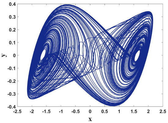
Figure 1.
When , chaos can be obtained in system (1) with initial values (−1.01,−0.01,−0.01).
3. Fractional-Order Model of Modified Chua’s Circuit
The Caputo method is one of the most common methods used in Solving the fractional-order systems numerically. However, the Grunwald–Letnikov (GL) method can be preferred for numerical solutions of the fractional-order systems because of the smoothness of the resultant approximations [19,20]. Thus, we choose the GL method in this section because of its iterative feature. The memory effect can be observed in the sum and binomial coefficients are defined recursively and have smooth properties. Using the continuous Riemann–Liouville method for the discretization of the fractional equations [21,22,23], the GL derivative can be used and requires a discrete convolution of binomial coefficient function and the function of interest. Here, the binomial coefficients are defined analytically [3]. Some related results can be found in refereces [24,25,26,27,28,29,30].
The definition of GL derivative is
and
where a and t represent the limits, represents generalized difference, h is the step size and q is the fractional-order. In order to limit the memory for binomial coefficients, short memory principle is used.
The binomial coefficients can be calculated as,
Below the 3D fractional-order Chua’s circuit general form is given.
The discretization method given in (7) is used to solve the system (6) numerically with GL method.
where is the binomial coefficients as given in (5). The N value is selected as L, that is the truncation window size or as k for all the used memory elements.
The definition of the autonomous fractional-order abs system (FOABS) is given below.
where and .
The N value is selected as L, that is the truncation window size or as k for all the used memory elements. When parameters or and commensurate fractional-order , the FOABS exhibits chaotic oscillations for the initial values of as shown in Figure 2.
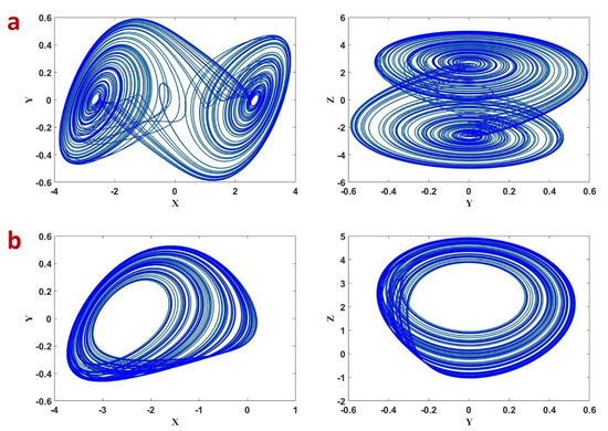
Figure 2.
Phase portraits of the fractional-order abs system (FOABS) (8) for (a) ; (b) .
4. Dynamical Properties of the FOABS System
4.1. Lyapunov Exponents
To find the Lyapunov Exponents (LEs) of the FOABS, the modified Wolf’s algorithm [31,32] is used. The LEs of the FOABS are found to be for the initial values , parameter values and fractional-order .
4.2. Route to Chaos
Bifurcation diagrams and dynamic behaviorof the FOABS are given in Figure 3 and Figure 4 with respect to the fractional-order q and parameter respectively. In Figure 3a the parameter while in Figure 3b the parameter . Figure 3a shows that the FOABS exhibits chaotic behavior for and Figure 3b shows that the system exhibits chaotic behavior for . It is obvious that the FOABS takes period doubling route to chaos. Figure 4 shows the bifurcation with parameter when the fractional-order , and the FOABS takes an inverse period doubling exit from chaos. For the Figure 3 and Figure 4, the other parameters are kept at .
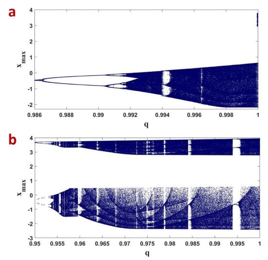
Figure 3.
The bifurcation of the FOABS (8) with respect to q for (a) ; (b) .
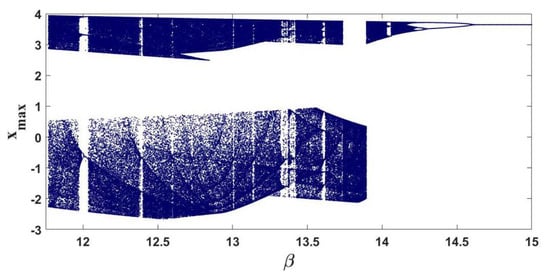
Figure 4.
Bifurcation of the FOABS system (8) with respect to for .
4.3. Multistability and Coexisting Attractors
The discontinuous bifurcations in Figure 3 and Figure 4 confirm that the FOABS system can show multistability and coexisting attractors. To investigate this the well-known forward and backward continuation are used [33]. In forward continuation, the parameter of interests is increased from minimum to maximum and initial values are initialized to the end values of state trajectories. Finally, the local maxima of the state variables are plotted. In backward continuation, the parameter of interests is decreased from maximum to minimum. The next steps are carried out as same as in forward continuation. Figure 5a shows the multistable plots of the FOABS with fractional-order q while the other parameters kept as . Blue plots show the forward continuation and red plots show the backward continuation. Similarly Figure 5b shows the bifurcation with respect to while other parameters kept as . and fractional-order . Red plots show the forward continuation and blue plots show the backward continuation. Figure 6 shows the coexisting attractors for different values of q and .
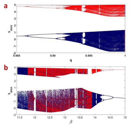
Figure 5.
(a) Bifurcation of the FOABS with respect to q (the blue plot is forward continuation and the red plot is backward continuation); (b) Bifurcation of the FOABS with respect to (the red plot is forward continuation and the blue plot is backward continuation).
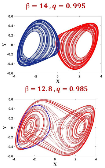
Figure 6.
The coexisting attractors shown by the FOABS system (8).
5. Microcontroller-Based Implementation of FOABS System
In this section, microcontroller-based circuit design of the FOABS system was implemented at ATmega328p microcontroller in Arduino UNO board to use in real digital engineering applications. Equation (9) is adapted to the microcontroller and microcontroller program was written in the Arduino v.1.8.9 compiler program. The flow chart of the microcontroller program is given in Figure 7. In the software, the initial values , fractional-order q value and parameters (a, b, , ) values of the FOABS system are first taken from the user via USB (Universal Serial Bus) communication with a computer. With these values, the FOAB system state variables are calculated and sent via USB port.
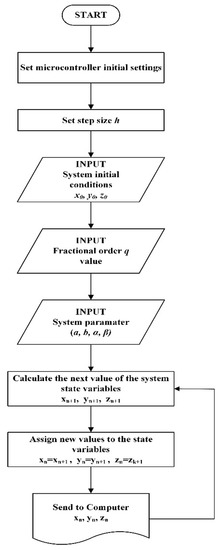
Figure 7.
The flow chart of the microcontroller program.
The designed system using the Arduino–Uno microcontroller platform is connected to the computer and testing was realized in Figure 8. The test parameters were taken as follows: step size and . An example screenshot of the communication between the microcontroller and the computer is given in Figure 9. The data coming from the microcontroller to the computer were drawn in Matlab (Figure 10). When Figure 2a and Figure 10 are examined together, it is seen that the results obtained with the microcontroller and the numerical simulation results confirm each other. Desired parameters can be easily changed in the designed microcontroller-based system. In this way, the FOABS system outputs can be obtained in a very flexible way with different parameter values.
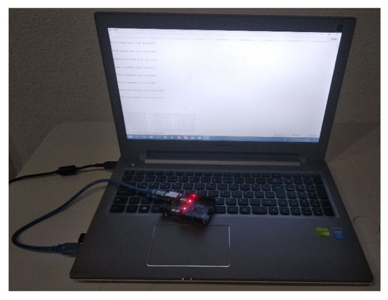
Figure 8.
Microcontroller-based system test platform.
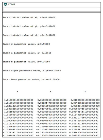
Figure 9.
An example screenshot of the communication between the microcontroller and the computer.
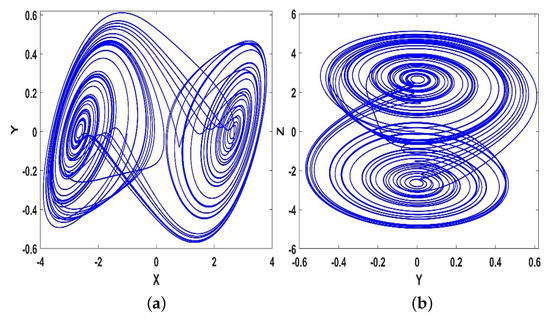
Figure 10.
2D phase portraits of the FOABS system obtained from the microcontroller, (a) ; (b) .
6. Electronic Circuit Realization of Modified Chua’s Circuit (1)
Recent years have seen rapid improvements in chaos science and also in studies on understanding chaos and chaotic systems, detecting features and differences, observing experimental data. Among such studies are chaotic circuit studies on modeling the chaotic systems [34,35,36]. In this section, the modeling of a chaotic system with absolute function is implemented in ORCAD-PSpice simulation environment.
The chaotic system’s electronic circuit with absolute function is realized in ORCAD-PSpice. The parameter values are set as and in electronic circuit implementation. Compared with the result in [16], Figure 11 has different components like inductor. In our design, there are two Op-amps for function, but function in [4] has four Op-amps for the circuit implementation. Select C1 = C2 = C3 = 1nF, R1 = 43 k, R2 = 259 k, R3 = 69 k, R4 = R5 = R9 = R10 = R12 = R13 = R14 = R15 = R16 = R17 = R18 = 100 k, R6 = R7 = R8 = 400 k, R11 = 28.5 k, R10 = 333 k. The ORCAD-PSpice simulation outputs, are seen in Figure 12 and Figure 13 with initial values (−1.01, −0.01, −0.01).
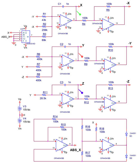
Figure 11.
The circuit schematic of the electronic design for system (1).
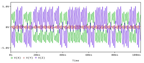
Figure 12.
Time series of the system (1) state variables.
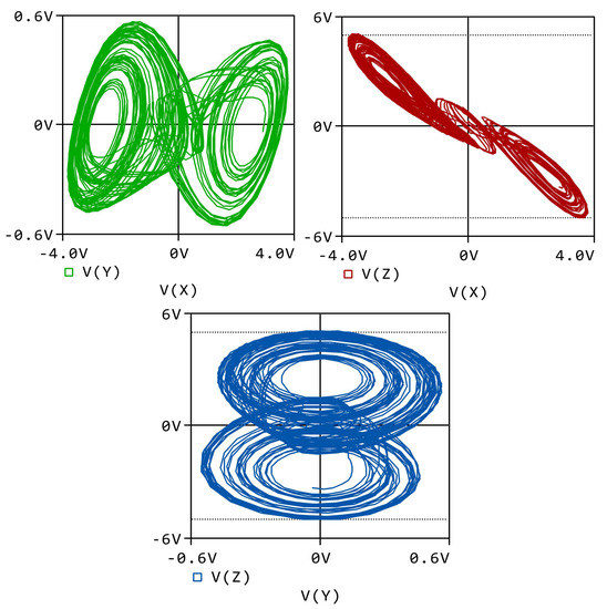
Figure 13.
The all phase portraits of electronic circuit design in ORCAD-PSpice for parameters and in system (1).
7. Conclusions
This paper considers the improved circuit implementation of the 3D Chua’s system with this function . In addition, analysis and microcontroller-based implementation of dynamical properties of the fractional-order form of this modified system is presented by bifurcation diagram, phase portrait, Lyapunov exponents, multistability and coexisting attractors. Using the designed microcontroller-based circuit of the FOABS system and electronic circuit implementation, this system can be used in various chaos-based real engineering applications such as encryption, random number generator and communication. More studies on possible applications of this research are planned in future works.
Author Contributions
Conceptualization, J.W. and A.A.; methodology, L.X.; software, K.R.; formal analysis, S.C. and B.A.; writing—original draft preparation, J.W. All authors have read and agreed to the published version of the manuscript.
Funding
This work is partially funded by Center for Nonlinear Systems, Chennai Institute of Technology, India vide funding number CIT/CNS/2020/RD/058.
Institutional Review Board Statement
Not applicable.
Informed Consent Statement
Informed consent was obtained from all subjects involved in the study.
Data Availability Statement
The study did not report any data.
Conflicts of Interest
The authors declare no conflict of interest.
References
- Lorenz, E.N. Deterministic nonperiodic flow. J. Atmos. Sci. 1963, 20, 130–141. [Google Scholar] [CrossRef]
- Rossler, O.E. An equation for continuous chaos. Phys. Rev. A 1976, 57, 397–398. [Google Scholar] [CrossRef]
- Chua, L.O.; Lin, G.N. Canonical realization of Chua’s circuit family. IEEE Trans. Circuits Syst. 1990, 37, 885–902. [Google Scholar] [CrossRef]
- Chen, G.; Ueta, T. Yet another chaotic attractor. Int. J. Bifur. Chaos 1999, 9, 1465–1466. [Google Scholar] [CrossRef]
- Leonov, G.A.; Kuznetsov, N.V. Hidden attractors in dynamical systems: From hidden oscillations in Hilbert-Kolmogorov, Aizerman, and Kalman problems to hidden chaotic attractor in Chua circuits. Int. J. Bifur. Chaos 2013, 23, 1330002. [Google Scholar] [CrossRef]
- Leonov, G.A.; Kuznetsov, N.V.; Vagaitsev, V.I. Ocalization of hidden Chua’s attractors. Phys. Lett. A 2011, 375, 2230–2233. [Google Scholar] [CrossRef]
- Leonov, G.A.; Kuznetsov, N.V.; Vagaitsev, V.I. Hidden attractor in smooth Chua systems. Phys. D Nonlinear Phenom. 2012, 241, 1482–1486. [Google Scholar] [CrossRef]
- Murillo-Escobar, M.A.; Cruz-Hernandez, C.; Abundiz-Perez, F.; Lopez-Gutierrez, R.M. Implementation of an improved chaotic encryption algorithm for real-time embedded systems by using a 32-bit microcontroller. Microprocess. Microsyst. 2016, 45, 297–309. [Google Scholar] [CrossRef]
- Janakiraman, S.; Thenmozhi, K.; Rayappan, J.B.B.; Amirtharajan, R. Lightweight chaotic image encryption algorithm forMicroprocess Microsystem, real-time embedded system: Implementation and analysis on 32-bit microcontroller. Microprocess. Microsyst. 2018, 56, 1–12. [Google Scholar] [CrossRef]
- Murillo-Escobar, M.A.; Cruz-Hernandez, C.; Abundiz-Perez, F.; Lopez-Gutierrez, R.M. A robust embedded biometric authentication system based on fingerprint and chaotic encryption. Expert Syst. Appl. 2015, 42, 8198–8211. [Google Scholar] [CrossRef]
- Kacar, S. Analog circuit and microcontroller based RNG application of a new easy realizable 4D chaotic system. Optik 2016, 127, 9551–9561. [Google Scholar] [CrossRef]
- Acho, L. discrete-time chaotic oscillator based on the logistic map: A secure communication scheme and a simple experiment using Arduino. J. Franklin Inst. 2015, 352, 3113–3121. [Google Scholar] [CrossRef]
- Ojo, K.S.; Adelakun, A.O.; Oluyinka, A.A. Synchronisation of cyclic coupled Josephson junctions and its microcontroller-based implementation. Pramana 2019, 92, 77. [Google Scholar] [CrossRef]
- Matouk, A.E.; Agiza, H.N. Bifurcations, chaos and synchronization in ADVP circuit with Parallel resistor. J. Math. Anal. Appl. 2008, 341, 259–269. [Google Scholar] [CrossRef]
- Agiza, H.N.; Matouk, A.E. Adaptive synchronization of Chua’s circuits with fully unknown parameters. Chaos Solitons Fractals 2006, 28, 219–227. [Google Scholar] [CrossRef]
- Tang, K.S.; Man, K.F.; Zhong, G.Q.; Chen, G.R. Modified Chua’s circuit with x|x|. Control Theory Appl. 2003, 20, 223–227. [Google Scholar]
- Tang, F.; Wang, L. An adaptive active control for the modified Chua’s circuit. Phys. Lett. A 2005, 346, 342–346. [Google Scholar] [CrossRef]
- Fu, S.; Meng, X.; Lu, Q. Stability and boundary equilibrium bifurcations of modified Chua’s circuit with smooth degree of 3*. Appl. Math. Mech. (Engl. Ed.) 2015, 36, 1639–1650. [Google Scholar] [CrossRef]
- Tolba, M.F.; AbdelAty, A.M.; Soliman, N.S.; Said, L.A.; Madian, A.H.; Azar, A.T.; Radwan, A.G. FPGA implementation of two fractional order chaotic systems. AEU-Int. J. Electron. Commun. 2017, 78, 162–172. [Google Scholar] [CrossRef]
- Petras, I. Fractional-Order Nonlinear Systems; Springer: Berlin/Heidelberg, Germany, 2011. [Google Scholar]
- MacDonald, C.L.; Bhattacharya, N.; Sprouse, B.P.; Silva, G.A. Efficient computation of the Grünwald-Letnikov fractional diffusion derivative using adaptive time step memory. J. Comput. Phys. 2015, 297, 221–236. [Google Scholar] [CrossRef]
- Yuste, S.B.; Acedo, L. On an explicit finite difference method for fractional diffusion equations. SIAM J. Numer. Anal. 2005, 42, 1862. [Google Scholar] [CrossRef]
- Podlubny, I. Fractional Differential Equations: An Introduction to Fractional Derivatives, Fractional Differential Equations, to Methods of Their Solution and Some of Their Applications; Academic Press: London, UK, 1998. [Google Scholar]
- El-Sayed, A.M.A.; Nour, H.M.; Elsaid, A.; Matouk, A.E.; Elsonbaty, A. Dynamical behaviors, circuit realization, chaos control and synchronization of a new fractional order hyperchaotic system. Appl. Math. Model. 2016, 40, 3516–3534. [Google Scholar] [CrossRef]
- El-Sayed, A.M.A.; Elsonbaty, A.; Elsadany, A.A.; Matouk, A.E. Dynamical analysis and circuit simulation of a new fractional-order hyperchaotic system and its discretization. Int. J. Bifurc. Chaos 2016, 26, 1650222. [Google Scholar] [CrossRef]
- Matouk, A.E. A novel fractional-order system: Chaos, hyperchaos and applications to linear control. J. Ournal. Appl. Comput. Mech. 2020. [Google Scholar] [CrossRef]
- Matouk, A.E.; Khan, I. Complex dynamics and control of a novel physical model using nonlocal fractional differential operator with singular kernel. J. Adv. Res. 2020, 24, 463–474. [Google Scholar] [CrossRef] [PubMed]
- Al-khedhairi, A.; Matouk, A.E.; Khan, I. Chaotic dynamics and chaos control for the fractional-order geomagnetic field model. Chaos Solitons Fractals 2019, 128, 390–401. [Google Scholar] [CrossRef]
- Rajagopal, K.; Karthikeyan, A.; Duraisamy, P.; Weldegiorgis, R.; Tadesse, G. Bifurcation, chaos and its control in a fractional order power system model with uncertainties. Asian J. Control. 2019, 21, 184–193. [Google Scholar] [CrossRef]
- Rajagopal, K.; Pham, V.T.; Alsaadi, F.E.; Alsaadi, F.E.; Karthikeyan, A.; Duraisamy, P. Multistability and coexisting attractors in a fractional order Coronary artery system. Eur. Phys. J. Spec. Top. 2018, 227, 837–850. [Google Scholar] [CrossRef]
- Wolf, A.; Swift, J.B.; Swinney, H.L.; Vastano, J.A. Determining Lyapunov exponents from a time series. Phys. D Nonlinear Phenom. 1985, 16, 285–317. [Google Scholar] [CrossRef]
- Danca, M.F. Lyapunov exponents of a class of piecewise continuous systems of fractional order. Nonlinear Dyn. 2015, 81, 227–237. [Google Scholar] [CrossRef]
- Hale, J.K. Forward and backward continuation for neutral functional differential equations. J. Differ. Equ. 1970, 9, 168–181. [Google Scholar] [CrossRef]
- Wei, Z.; Moroz, I.; Sprott, J.C.; Akgul, A.; Zhang, W. Hidden hyperchaos and electronic circuit application in a 5D self-exciting homopolar disc dynamo. Chaos Interdiscip. J. Nonlinear Sci. 2017, 27, 033101. [Google Scholar] [CrossRef] [PubMed]
- Volos, C.; Akgul, A.; Pham, V.-T.; Stouboulos, I.; Kyprianidis, I. A simple chaotic circuit with a hyperbolic sine function and its use in a sound encryption scheme. Nonlinear Dyn. 2017, 89, 1047–1061. [Google Scholar] [CrossRef]
- Pham, V.-T.; Akgul, A.; Volos, C.; Jafari, S.; Kapitaniak, T. Dynamics and circuit realization of a no-quilibrium chaotic system with a boostable variable. AEU-Int. J. Electron. Commun. 2017, 78, 134. [Google Scholar] [CrossRef]


Publisher’s Note: MDPI stays neutral with regard to jurisdictional claims in published maps and institutional affiliations. |
© 2021 by the authors. Licensee MDPI, Basel, Switzerland. This article is an open access article distributed under the terms and conditions of the Creative Commons Attribution (CC BY) license (http://creativecommons.org/licenses/by/4.0/).