Nonlinear Dynamics of Wave Packets in Tunnel-Coupled Harmonic-Oscillator Traps

Abstract

We consider a two-component linearly coupled system with the intrinsic cubic nonlinearity and the harmonic-oscillator (HO) confining potential. The system models binary settings in BEC and optics. In the symmetric system, with the HO trap acting in both components, we consider Josephson oscillations (JO) initiated by an input in the form of the HO’s ground state (GS) or dipole mode (DM), placed in one component. With the increase of the strength of the self-focusing nonlinearity, spontaneous symmetry breaking (SSB) between the components takes place in the dynamical JO state. Under still stronger nonlinearity, the regular JO initiated by the GS input carries over into a chaotic dynamical state. For the DM input, the chaotization happens at smaller powers than for the GS, which is followed by SSB at a slightly stronger nonlinearity. In the system with the defocusing nonlinearity, SSB does not take place, and dynamical chaos occurs in a small area of the parameter space. In the asymmetric half-trapped system, with the HO potential applied to a single component, we first focus on the spectrum of confined binary modes in the linearized system. The spectrum is found analytically in the limits of weak and strong inter-component coupling, and numerically in the general case. Under the action of the coupling, the existence region of the confined modes shrinks for GSs and expands for DMs. In the full nonlinear system, the existence region for confined modes is identified in the numerical form. They are constructed too by means of the Thomas–Fermi approximation, in the case of the defocusing nonlinearity. Lastly, particular (non-generic) exact analytical solutions for confined modes, including vortices, in one- and two-dimensional asymmetric linearized systems are found. They represent bound states in the continuum.

1. Introduction

The combination of a harmonic-oscillator (HO) trapping potential and cubic nonlinearity is a ubiquitous setting which occurs in diverse microscopic, mesoscopic, and macroscopic physical settings. A well-known realization is offered by Bose-Einstein condensates (BECs) with collisional nonlinearity [1,2,3], loaded in a magnetic or optical trap—see, e.g., Refs. [4,5,6,7,8,9,10,11,12,13,14]. A similar combination of the effective confinement, approximated by the parabolic profile of the local refractive index, and the Kerr term is relevant as a model of optical waveguides [15,16,17,18]. Models of the same type appear in other physical systems too, such as networks of Josephson oscillators [19].

The character of states created by the interplay of the intrinsic nonlinearity and externally applied trapping potential strongly depends on the sign of the nonlinearity. In the case of the self-attraction (or self-phase-modulation, SPM, in terms of optics [20]), localized modes, similar to solitons, arise spontaneously. On the other hand, self-repulsion tends to create flattened configurations, which, in turn, may support dark solitons in various static and dynamical states [6,7,8,9,10,11,12,13,14]. A specific situation occurs in a system combining repulsion and a weak parabolic potential with an additional spatially periodic one (it represents an optical lattice in BEC [21], or a photonic crystal in optics and plasmonics [22,23,24]): the interplay of the periodic potential with the self-repulsion gives rise to bright gap solitons [21,25], whose effective mass is negative. For this reason, gap solitons are expelled by the HO potential, but are trapped by the inverted one that would expel modes with positive masses [26].

Another noteworthy feature of the dynamics of one-dimensional (1D) nonlinear fields trapped in confining potentials is the degree of its nonintegrability. The generic model for such settings is provided by the nonlinear Schrödinger equation (NLSE, alias the Gross–Pitaevskii equation, in terms of BEC [1,2,3]) with the cubic term, whose integrability in the 1D space [27] is broken by the presence of the HO potential. Nevertheless, systematic numerical simulations, performed for the repulsive sign of the cubic nonlinearity, have demonstrated that the long-time evolution governed by NLSE with the HO potential term does not lead to establishment of spatiotemporal chaos (“turbulence”), which would be expected in the case of generic nonintegrability [28,29]. Instead, the setup demonstrates quasi-periodic evolution, represented by a quasi-discrete power spectrum, in terms of a multi-mode truncation (Galerkin approximation) [14]. This observation is specific for the harmonic (quadratic) confining potential, while anharmonic ones quickly lead to the onset of clearly observed chaos [30,31]. Thermalization of the model with the HO potential was recently explored, in the framework of a stochastically driven dissipative Gross–Pitaevskii equation, in Ref. [32].

The interplay of the cubic nonlinearity and trapping potentials also occurs in two-component systems, which represent, in particular, binary BEC [12,33,34,35]. Here, we aim to consider the system with linear coupling between the components. In optics, if two modes carrying orthogonal polarizations of light propagate in the same waveguide, linear mixing between them is induced by a twist of the guiding structure, see, e.g., Ref. [36]. In BEC, different atomic states which correspond to the interacting components can be linearly coupled by a resonant electromagnetic wave [37,38,39,40]. Another realization of linearly mixed systems is offered by dual-core waveguides, coupled by tunneling of the field across a barrier separating the cores. The dual-core schemes are equally relevant to optics and BEC [41]. In particular, experiments with temporal solitons in dual-core optical fibers were reported in recent work [42].

The coupling between the components enhances the complexity of the system and makes it possible to find new static and dynamical states in it. In particular, the symmetric system combining the attractive cubic terms of the SPM type and (optionally) HO potential acting in each component, with linear coupling between them, gives rise to spontaneous symmetry breaking (SSB) of two-component states [35,42]. In the case of repulsive SPM acting in each component and nonlinear repulsion between them (cross-phase modulation, XPM), it was found [33] that the linear mixing shifts the miscibility-immiscibility transition [43] in the trapped condensate. Furthermore, effects of nonintegrability may be stronger in the linearly coupled system, because the linear coupling makes the system of one-dimensional NLSEs nonintegrable, even in the absence of the HO potential [44], although the integrability is kept by the system with the linear coupling added to the SPM and XPM terms with equal strengths (the Manakov’s nonlinearity) [45].

The objective of the present work is two-fold. First, in Section 2 we aim to analyze the onset of chaos, as well as SSB, in the symmetric linearly coupled system, with both attractive and repulsive signs of the SPM terms, starting from an input in the form of the ground state (GS), or the first excited state (the dipole mode (DM), represented by a spatially odd wave function) of the HO, which is initially launched in one core (component), while the other one is empty. This type of the input is, in particular, experimentally relevant in optics [42]. As a nonchaotic dynamical regime in this case, one may expect Josephson oscillations (JO) of the optical field [42,44,46,47,48,49], or of the BEC wave function [50,51,52,53,54,55,56], between the cores. As a measure of the transition to dynamical chaos in the system, we use a relative spread of the power spectrum of oscillations produced by simulations of the coupled NLSEs. Naturally, the chaotization sets in above a certain threshold value of the nonlinearity strength, and the chaos is much weaker in the case of the repulsive nonlinearity. In the dynamical state initiated by the GS, the SSB takes place prior to the onset of the dynamical chaos, while the DM input undergoes the chaotization occurs first, followed by the SSB at a slightly stronger nonlinearity.

The second objective, which is presented below in Section 3, is to construct stationary GS and DM in the asymmetric (half-trapped) linearly coupled system, with the HO potential applied to one component only. The latter system can be realized in the experiment, applying, for instance, the trapping potential only to one core of the double waveguide for matter waves in BEC (e.g., by focusing laser beams, which induce the trapping, on the single core). In optics, a similar setup may be built as a coupler with two widely different cores, narrow and broad ones, with the narrow core emulating the component carrying a tightly confining potential, cf. Ref. [57]. A remarkable peculiarity of such a system is that the linear coupling mixes completely different types of the asymptotic behavior at $\left|x\right|\to \infty$: the trapped component is always confined, in the form of a Gaussian, by the HO potential, while the untrapped one is free to escape. In addition, the asymmetry between the coupled cores makes it necessary to take into regard a difference in the chemical potentials or propagation constants (in terms of the BEC and optics, respectively) between them, which is represented by parameter $\omega$ in Equation (10), see below. Some results for the half-trapped system are obtained in an analytical form, in the weak- and strong-coupling limits, as well as by means of the Thomas–Fermi approximation (TFA), and full results are produced numerically. In addition, particular solutions for localized states of the linear half-trapped system (including vortex states in its 2D version) are found in an exact form. The exact solutions belong to the class of bound states in the continuum [58,59,60], alias embedded [61] ones, which are spatially confined modes existing, as exceptional states, with the carrier frequency falling in the continuous spectrum. The paper is concluded by Section 4.

2. The Symmetric System

2.1. The Coupled Equations

As outlined above, we consider systems modeled by a pair of coupled NLSEs for complex amplitudes $u\left(x,z\right)$ and $v\left(x,z\right)$ of two interacting waves. In the normalized form, the equations are written in terms of the spatial-domain propagation in an optical waveguide with propagation distance z and transverse coordinate x:

$$\begin{array}{ccc}\hfill i\frac{\partial u}{\partial z}+\frac{1}{2}\frac{{\partial }^{2}u}{\partial x^2}+\lambda v-\frac{{\mathsf{\Omega }}^2}{2}{x}^{2}u+\sigma \left({\left|u\right|}^2+g{\left|v\right|}^2\right)u& =& 0,\hfill \\ & & \hfill \\ \hfill i\frac{\partial v}{\partial z}+\frac{1}{2}\frac{{\partial }^{2}v}{\partial x^2}+\lambda u-\frac{{\mathsf{\Omega }}^2}{2}{x}^{2}v+\sigma \left({\left|v\right|}^2+g{\left|u\right|}^2\right)v& =& 0.\hfill \end{array}$$

(1)

Here, coefficients $\sigma >0$ or $\sigma <0$ represents the strength of the focusing or defocusing SPM in each core, while $\lambda$ and $\sigma g$ represent the linear mixing and XPM interaction, respectively. By means of rescaling, the strength of the HO trapping potential is set to be $\mathsf{\Omega }=1$ (unless it is zero in one core). In other words, x is measured in units of the respective HO length. This implies that the unit of the transverse coordinate in the optical waveguides takes typical values in the range of 10–30 $\mathsf{\mu }$m, hence the respective unit of the propagation distance (the Rayleigh/diffraction distance corresponding to the OH length) is estimated to be between 1 mm and 1 cm, for the carrier wavelength $\sim 1$ μm. In the matter-wave realization of the system, typical units of x and time (replacing z in Equation (1) are $\sim 10$ μm and 10 ms, respectively.

The system conserves two dynamical invariants., viz., the total norm (or power, in terms of optics),

$$P={\int }_{-\infty }^{+\infty }\left[{\left|u\left(x\right)\right|}^2+{\left|v\left(x\right)\right|}^2\right]dx,$$

(2)

and the Hamiltonian (in which $\mathsf{\Omega }=1$ is set),

$$\begin{array}{c}H={\int }_{-\infty }^{+\infty }\left[\frac{1}{2}\left({\left|\frac{{\partial }^{2}u}{\partial x^2}\right|}^2+{\left|\frac{{\partial }^{2}v}{\partial x^2}\right|}^2\right)-\frac{\sigma }{2}\left({\left|u\right|}^4+{\left|v\right|}^4\right)\right.\\ \left.-{\sigma g\left|u\right|}^2{\left|v\right|}^2+\frac{1}{2}{x}^2\left({\left|u\right|}^2+{\left|v\right|}^2\right)-\lambda \left(u{v}^{\ast }+u^{\ast }v\right)\right]dx,\end{array}$$

(3)

where * stands for the complex conjugate. The remaining scaling invariance of Equation (1) makes it possible to either set $\left|\sigma \right|=1$, or keep nonlinearity coefficient $\sigma$ as a free parameter, but fix $P\equiv 1$. All simulations performed in this work comply with the conservation of P and H, up to the accuracy of the numerical codes.

It is relevant to mention that the present two-component system resembles nonlinear models with a double-well potential, in the case when the wave functions in two wells are linearly coupled by tunneling across the potential barrier, see, e.g., Refs. [62,63]. Nevertheless, the exact form of the system and its solutions are different.

In the limit of a small amplitude $A_0$ of the input, linearized Equation (1) with $\mathsf{\Omega }=1$ admit exact solutions for inter-core JO of the ground and dipole states (exact solutions for higher-order states can be readily found too):

$$\begin{array}{ccc}\hfill u_{\mathrm{JO}}^{\left(\mathrm{GS}\right)}\left(x,t\right)& =& A_{0}exp\left(-\frac{1}{2}{x}^2-\frac{1}{2}iz\right)cos\left(\lambda z\right),\hfill \\ & & \hfill \\ \hfill v_{\mathrm{JO}}^{\left(\mathrm{GS}\right)}\left(x,t\right)& =& i{A}_{0}exp\left(-\frac{1}{2}{x}^2-\frac{1}{2}iz\right)sin\left(\lambda z\right),\hfill \end{array}$$

(4)

$$\begin{array}{ccc}\hfill u_{\mathrm{JO}}^{\left(\mathrm{DM}\right)}\left(x,t\right)& =& A_{0}xexp\left(-\frac{1}{2}{x}^2-\frac{3}{2}iz\right)cos\left(\lambda z\right),\hfill \\ & & \hfill \\ \hfill v_{\mathrm{JO}}^{\left(\mathrm{DM}\right)}\left(x,t\right)& =& i{A}_{0}xexp\left(-\frac{1}{2}{x}^2-\frac{3}{2}iz\right)sin\left(\lambda z\right).\hfill \end{array}$$

(5)

Expressions given by Equations (4) and (5) at $z=0$ are used below as inputs in simulations of the full nonlinear Equation (1). The simulations presented in this section were performed in domain $\left|x\right|<10$. This size, tantamount to 20 HO lengths, is sufficient to display all details of the solutions. Standard numerical methods were used, viz., the split-step fast-Fourier-transform scheme for simulations of the evolution governed by Equations (1) and (10), and the relaxation algorithm for finding solutions to stationary equations, such as Equations (12) and (13), see below.

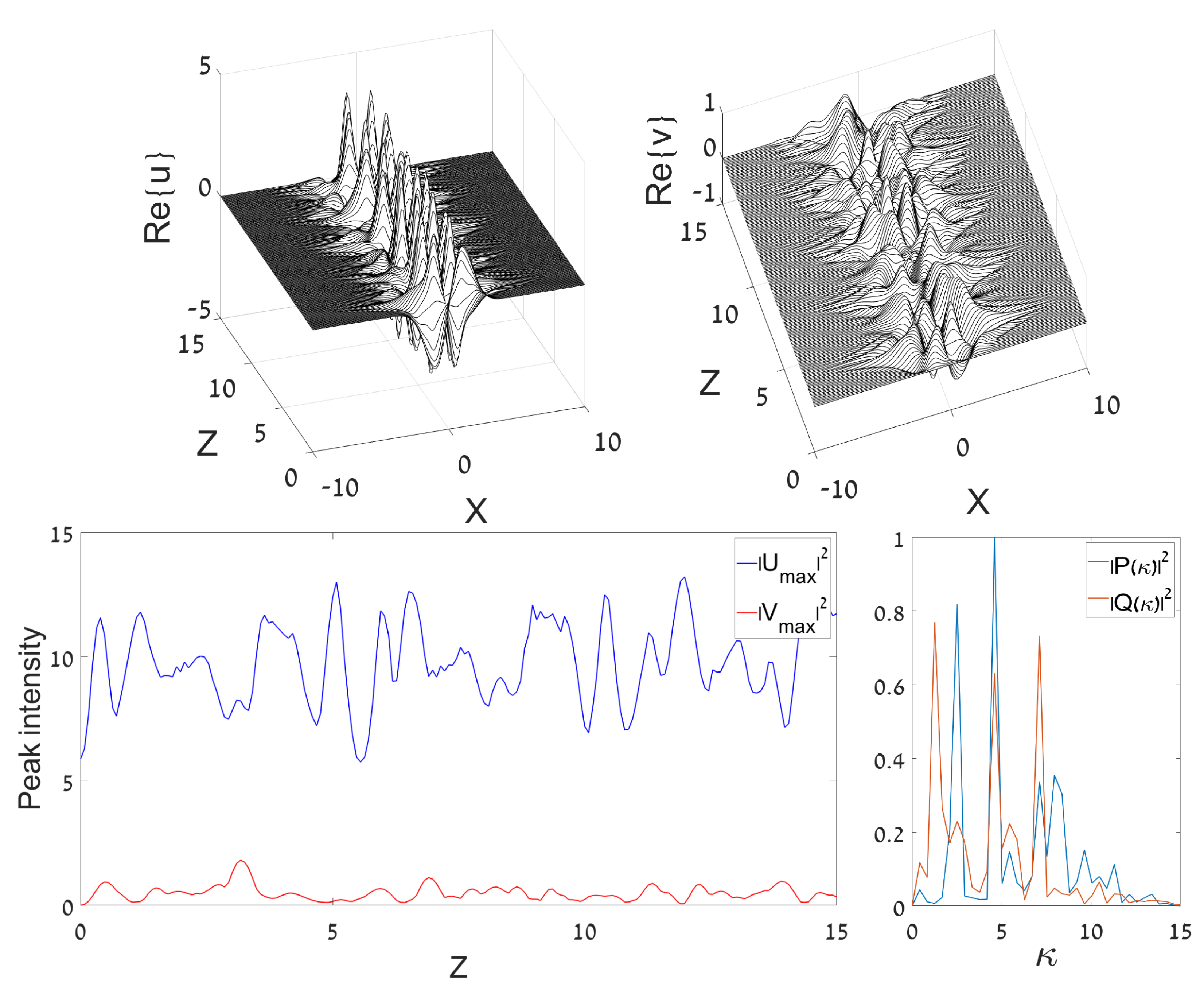
2.2. The Transition from Regular to Chaotic Dynamics

Increase of amplitude $A_0$ of the input leads to nonlinear deformation of the oscillations, and eventually to the onset of dynamical chaos. A typical example of an essentially nonlinear but still regular JO dynamical regime, produced by numerical simulations of Equation (1) with $g=0$ (no XPM interaction), in interval $0<z<Z$, with the DM input, taken as per Equation (5) at $z=0$, is presented in Figure 1. In particular, the left bottom panel of the figure displays oscillations of peak intensities of the fields,

$$\left\{U_{max}^2\left(z\right),V_{max}^2\left(z\right)\right\}\equiv \underset{x}{max}\left\{{\left|u(x,z)\right|}^2,{\left|v(x,z)\right|}^2\right\},$$

(6)

and, as a characteristic of the dynamics, in the right bottom panel we plot power spectra, ${\left|P\left(\kappa \right)\right|}^2,{\left|Q\left(\kappa \right)\right|}^2$, produced by the Fourier transform of the peak intensities:

$$\left\{P\left(\kappa \right),Q\left(\kappa \right)\right\}={\int }_0^Z\left\{U_{max}^2\left(z\right),V_{max}^2\left(z\right)\right\}exp\left(-i\kappa z\right)dz,$$

(7)

where $\kappa$ is a real propagation constant. Very slow decay of the peak intensities, observed in the former panel, is a manifestation of the system’s nonintegrability (in this connection, we again stress that the total norm is conserved during the simulations).

The regularity of the dynamical regime displayed in Figure 1 is clearly demonstrated by its spectral structure, which exhibits a single narrow peak at ${\kappa }_{\mathrm{peak}}\approx 2$. The peak’s width, $\Delta \kappa \simeq 0.1$, which corresponds to the relative width, $\Delta \kappa /{\kappa }_{\mathrm{peak}}\approx 0.05$, is comparable to the spread of the Fourier transform, corresponding to $Z=100$ in Figure 1. It can be estimated as $\delta \kappa =2\pi /Z\approx 0.06$. Note the overall symmetry between the two components in Figure 1 (in particular, their spectra are identical in the bottom panel).

The simulations with the same input, but larger values of $A_0$, give rise to chaotic (“turbulent”) dynamical states with a broad dynamical spectrum, see a typical example in Figure 2. Note that both the regular and chaotic dynamical pictures displayed in Figure 1 and Figure 2 extend over the distance estimated to be ∼10 Rayleigh (diffraction) lengths corresponding to the width of the DM input. This estimate is sufficient to make conclusions about the character of the dynamics.

Systematic simulations with the GS input, provided by Equation (4) at $z=0$, produce similar results (not shown here in detail). In particular, as well as in the case of the DM input, amplitudes $A_0=1$ and 4 initiate, severally, quasi-regular and chaotic evolution.

The results for the transition from regular JO to chaotic dynamics, initiated by the GS and DM inputs, taken as per Equations (4) and (5) at $z=0$, are summarized in charts plotted in the plane of $\left(\lambda ,A_0^2\right)$ in Figure 3. They display heatmaps of values of the parameter which quantifies the sharpness of the central peak in the spectrum of the dynamical state:

$$\mathrm{Sharpness}\equiv \frac{{\int }_{\mathrm{FWHM}}{\left|P\left(\kappa \right)\right|}^{2}d\kappa }{{\int }_0^{\infty }{\left|P\left(\kappa \right)\right|}^{2}d\kappa },$$

(8)

where the integration in the numerator is performed over the section of the central spectral peak selected according to the standard definition of the full width at half-maximum: ${\left|P\left({\kappa }_{\mathrm{FWHM}}\right)\right|}^2=(1/2){\left(P\left(\kappa \right)\right)}_{max}$. Values of $\mathrm{Sharpness}$ close to 1 imply the domination of a single sharp peak, such as one in Figure 1, which corresponds to a regular dynamical regime, while decrease of this parameter indicates a transition to a broad spectrum, which is a telltale of the onset of chaotic dynamics—see, e.g., Figure 2.

Figure 3 clearly demonstrates decay of the central peak’s sharpness, i.e., transition to dynamical chaos, with the increase of the input’s intensity, $A_0^2$, in the case of the attractive SPM, $\sigma =+1$. Such a trend is not straightforward in the opposite case of the self-repulsion, $\sigma =-1$. In particular, the chaotization is not observed at all in the latter case at small values of $\lambda$. This conclusion agrees with findings reported in work [14] for the single-component NLSE (which corresponds to $\lambda =0$), with the HO potential and $\sigma =-1$. Computations of the spectrum, reported in that work, demonstrate that no transition to dynamical chaos takes place at all values of parameters. The fact that an area of weak chaotization is, nevertheless, observed in the right panels of Figure 3 is explained by the above-mentioned circumstance, that the addition of the linear coupling to a pair of NLSEs destroys their integrability (in free space). On the other hand, the increase of the sharpness with the increase of $\lambda$, observed at relatively small values of $A_0^2$ (which is observed in an especially salient form in the left bottom panel of Figure 3) also has a simple explanation: the increase of $\lambda$ makes the linear terms in the system dominating over nonlinear ones, thus tending to maintain a quasi-linear behavior.

Lastly, the comparison of the left and right panels in Figure 3 suggests that the chaotization sets in faster in dynamical regimes initiated by the DM input, in comparison to their counterparts originating from the GS, for the same values of the input’s intensity, $A_0^2$. The difference between the GS and DM dynamical regimes is salient for relatively small values of $\lambda$. It may be explained by the fact that attractive SPM naturally tends to form a stable bright soliton from the GS input, which then maintains regular motion in the HO potential [64]. On the other hand, spatially odd bright solitons do not exist in free space, which impedes transformation of the DM input into a regular dynamical state.

As said above, the heatmaps are displayed in Figure 3 for $g=0$, i.e., in the absence of the XPM coupling between the components, which is the case for dual-core couplers. On the other hand, in the case of the Manakov’s nonlinearity, i.e., $g=1$, the above-mentioned integrability of such a system of NLSEs with the linear coupling [45] (but without the trapping potential) suggests that the full system will be closer to integrability and farther from the onset of chaos. Indeed, numerical results collected from simulations of Equation (1) with $\sigma =g=+1$ (not shown here in detail) demonstrate a much smaller chaotic area in the $\left(\lambda ,A_0^2\right)$ plane. In particular, the GS input generates “turbulent” behavior only at $A_0^2\gtrsim 200$, being limited to $\lambda \lesssim 0.15$, cf. the top left panel in Figure 3.

2.3. Spontaneous Symmetry Breaking (SSB) between the Coupled Components

A noteworthy feature of the dynamical state presented in Figure 2 is breaking of the symmetry between fields u and v (while the patterns initiated by the GS and DM inputs keep their parities, i.e., spatial symmetry (evenness) and antisymmetry (oddness), respectively). This is a manifestation of the general effect, which is well known, in diverse forms, in linearly coupled dual-core systems with intrinsic attractive SPM [41]. In particular, SSB of stationary states in systems with the HO trapping potential acting in both cores was addressed in Refs. [35,56], while Figure 2 demonstrates the symmetry breaking in the dynamical JO state.

The SSB effect may be quantified, as usual [44], by asymmetry of the dynamical states, which we define as

$$\mathsf{\Theta }\equiv \frac{{\int }_0^{\infty }{\left|P\left(\kappa \right)\right|}^{2}d\kappa -{\int }_0^{\infty }{\left|Q\left(\kappa \right)\right|}^{2}d\kappa }{{\int }_0^{\infty }{\left|P\left(\kappa \right)\right|}^{2}d\kappa +{\int }_0^{\infty }{\left|Q\left(\kappa \right)\right|}^{2}d\kappa }.$$

(9)

The SSB occurs as a transition from $\mathsf{\Theta }=0$ to $\mathsf{\Theta }\ne 0$ with the increase of $A_0^2$ at some critical point, which is a generic property of stationary states in dual-core systems with intrinsic attractive nonlinearity [41,44], while here we consider it in the dynamical setting. On the other hand, in the case of the repulsive nonlinearity, $\sigma =-1$ in Equation (1), SSB of stationary states takes place in this system only at $g>1$ [56], while we here focus on the most relevant case of $g=0$. Accordingly, the present system with $\sigma =-1$ does not feature SSB.

For $\sigma =+1$, the SSB boundaries in the parameter planes of the GS and DM solutions are shown by bold black lines in the top and bottom left panels of Figure 3, respectively. The SSB bifurcation of the dynamical states under consideration is of the supercritical, alias forward, type [65], in terms of dependence $\mathsf{\Theta }\left(A_0^2\right),$ as shown in Figure 4 for the dynamical states initiated by the GS and DM inputs. It is observed that, naturally, the critical value of $A_0^2$ increases with $\lambda$, as the symmetry is maintained by the linear coupling, hence stronger coupling needs stronger nonlinearity to break the symmetry. Note also that the transition from $\mathsf{\Theta }=0$ to $\mathsf{\Theta }\approx 1$ (a strongly asymmetric state) is steeper at larger $\lambda$.

It is worth noting that, as clearly shown by the SSB boundary (the black line) in the top left panel of Figure 3, the SSB of the GS mode happens prior to the transition to the dynamical chaos. This conclusion agrees with known results showing that SSB of stationary modes does not, normally, lead to chaotization of the system’s dynamics [41,44]. On the other hand, the bottom left panel in Figure 3 demonstrates a different situation for the DM states, which exhibit the chaotization prior to the SSB, although the separation between these transitions is small. This conclusion agrees with the fact that, as clearly seen in Figure 4, the SSB in DM states occurs at values of the input’s amplitude essentially higher than those which determine the SSB threshold of the GS solutions.

3. The Half-Trapped System

The asymmetric system of linearly coupled NLSEs, with the HO potential included in one equation only, is written as

$$\begin{array}{ccc}\hfill i{u}_z+\frac{1}{2}{u}_{xx}+\lambda v-\frac{1}{2}{x}^{2}u+\sigma \left({\left|u\right|}^2+g{\left|v\right|}^2\right)u& =& -\omega u,\hfill \\ & & \hfill \\ \hfill i{v}_z+\frac{1}{2}{v}_{xx}+\lambda u+\sigma \left({\left|v\right|}^2+g{\left|u\right|}^2\right)v& =& 0,\hfill \end{array}$$

(10)

cf. Equation (1). Here, as said above, $\mathsf{\Omega }=1$ is set in the first equation, and the propagation-constant mismatch, $\omega$ (in terms of BEC, it represents a difference in the chemical potentials between the two wave functions) is a common feature of asymmetric systems. Stationary solutions to Equation (10) are looked for as

$$\left\{u,v\right\}=\left\{U\left(x\right),V\left(x\right)\right\}exp\left(-i\mu z\right),$$

(11)

with real propagation constant $-\mu$ (in BEC, with z replaced by t, $\mu$ is the chemical potential), and real functions $U\left(x\right)$ and $V\left(x\right)$ satisfying equations

$$\begin{array}{c}\left(\mu +\omega \right)U+\frac{1}{2}\frac{d^{2}U}{d{x}^2}+\lambda V-\frac{1}{2}{x}^{2}U+\sigma \left(U^2+g{V}^2\right)U=0,\end{array}$$

(12)

$$\begin{array}{c}\mu V+\frac{1}{2}\frac{d^{2}V}{d{x}^2}+\lambda U+\sigma \left(V^2+g{U}^2\right)V=0.\end{array}$$

(13)

Most results are produced below disregarding the XPM coupling between the components ($g=0$). Nevertheless, the XPM terms are included when collecting numerical results for the threshold of the existence of bound states.

3.1. The Linearized System: Analytical and Numerical Results

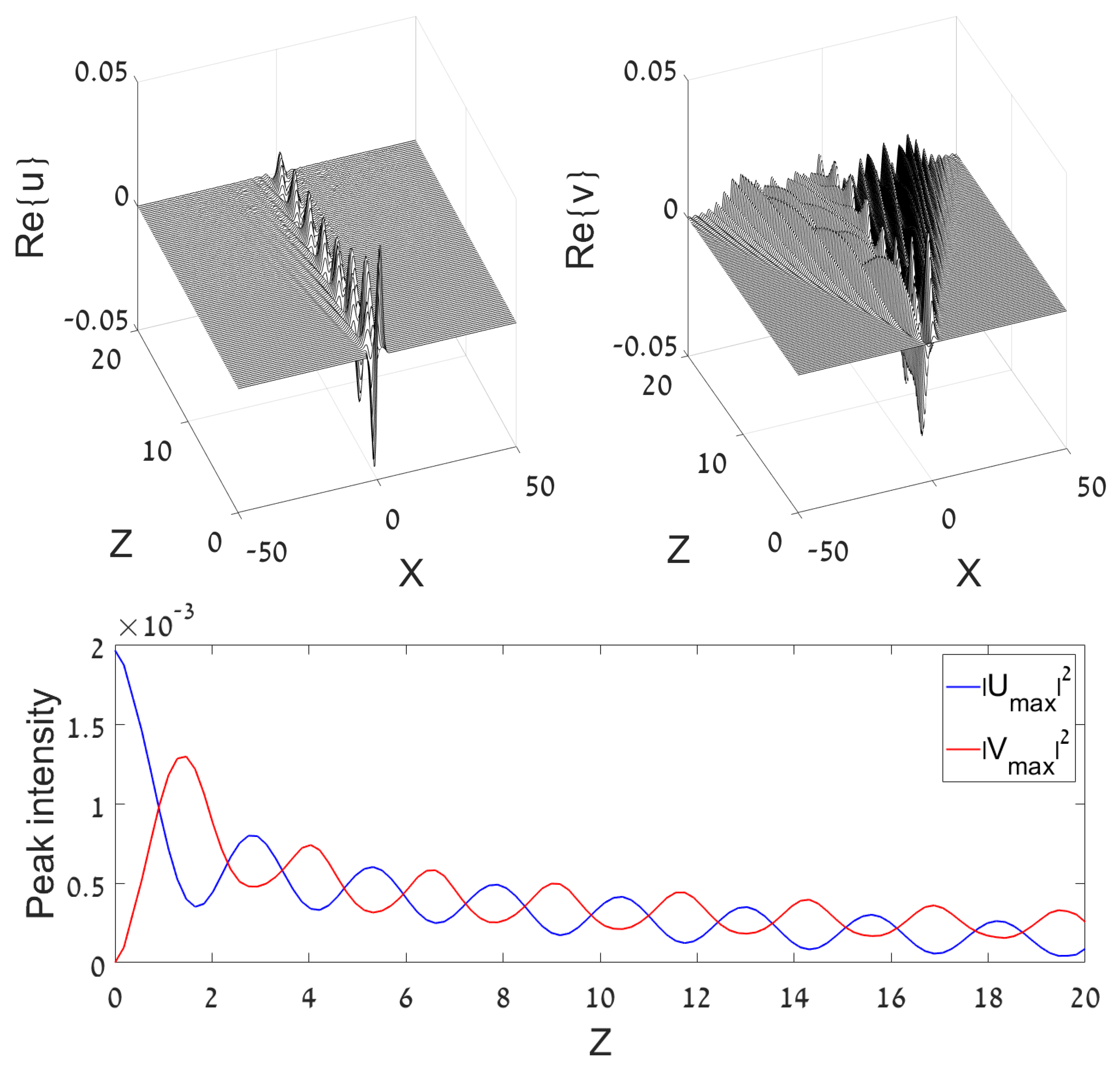
3.1.1. Emission of Radiation in the Untrapped Component

In the linear limit, $\sigma =0$, two decoupled equations in system (10) with $\lambda =0$ produce completely different results: all excitations of component u stay confined in the HO trap, while the v component with any $\mu >-\omega$ freely expands. In particular, in the limit of $\lambda =0$, obvious bound-state GS and DM solutions to the linearized version of Equations (12) and (13), with zero v component, are

$$\begin{array}{ccc}\hfill U_{\mathrm{GS}}^{\left(0\right)}\left(x\right)& =& \frac{1}{{\pi }^{1/4}}exp\left(-\frac{x^2}{2}\right),V_{\mathrm{GS}}^{\left(0\right)}=0,\hfill \end{array}$$

(14)

$$\begin{array}{ccc}\hfill U_{\mathrm{DM}}^{\left(0\right)}\left(x\right)& =& \frac{\sqrt{2}}{{\pi }^{1/4}}xexp\left(-\frac{x^2}{2}\right),V_{\mathrm{DM}}^{\left(0\right)}=0,\hfill \end{array}$$

(15)

where the pre-exponential constants are determined by the normalization condition,

$${\int }_{-\infty }^{+\infty }\left[U^2\left(x\right)+V^2\left(x\right)\right]dx=1,$$

(16)

which we adopt in this section. The eigenvalues corresponding to eigenmodes (14) and (15) are

$${\mu }_{\mathrm{GS}}^{\left(0\right)}=1/2-\omega ;{\mu }_{\mathrm{DM}}^{\left(0\right)}=3/2-\omega .$$

(17)

Proceeding to dynamical states, in the lowest approximation with respect to small $\lambda$ the evolution of the v field is driven by the respective linearized equation in system (10),

$$i{v}_z+\frac{1}{2}{v}_{xx}=-\lambda U_{\mathrm{GS},\mathrm{DM}}^{\left(0\right)}\left(x\right)exp\left(-i{\mu }_{\mathrm{GS},\mathrm{DM}}^{\left(0\right)}z\right).$$

(18)

Obviously, Equation (18) gives rise to emission of propagating waves (“radiation”), in the form of $v\sim \lambda exp\left(ikx-i{\mu }_{\mathrm{GS},\mathrm{DM}}^{\left(0\right)}z\right)$, at resonant wavenumbers $k=\pm \sqrt{2{\mu }_{\mathrm{GS},\mathrm{DM}}^{\left(0\right)}}$, provided that ${\mu }_{\mathrm{GS},\mathrm{DM}}^{\left(0\right)}$ is positive, i.e.,

$$v_{\mathrm{rad}}\sim \lambda exp\left(\pm i\sqrt{2{\mu }_{\mathrm{GS},\mathrm{DM}}^{\left(0\right)}}\left(x-V_{\mathrm{ph}}z\right)\right),$$

(19)

where the phase velocity is

$$V_{\mathrm{ph}}=\frac{k}{2}\equiv \pm \frac{1}{2}\sqrt{2{\mu }_{\mathrm{GS},\mathrm{DM}}^{\left(0\right)}}$$

(20)

(in terms of the spatial-domain propagation in the optical waveguide, it is actually the beam’s slope). The expansion of the area in the $\left(x,z\right)$ plane occupied by the radiation field is bounded by the group velocity, $\left|V_{\mathrm{gr}}\right|=\left|k\right|\equiv 2V_{\mathrm{ph}}$.

An illustration of this dynamics is presented in Figure 5. Straight red lines designate the wave-propagation directions, which exactly agree with the phase velocity predicted by Equation (20), and the expansion of the area occupied by the radiation complies with the prediction based on the group velocity.

The emission of radiation into the v core gives rise to a gradual decay of the amplitude in the u core, due to the conservation of the total norm, see Equation (16). An example of the decay is displayed in Figure 6, for a small initial amplitude of the GS input, $A_0=0.1$ (which corresponds to the quasi-linear dynamical regime), and a relatively large coupling constant, $\lambda =1$, which makes the transfer of the norm (power) from u to v faster.

On the other hand, the same input with large $A_0$ makes the u-v coupling a weak effect, in comparison with the dominant nonlinearity, hence the input mode in the u core seems quite stable, as shown in Figure 7.

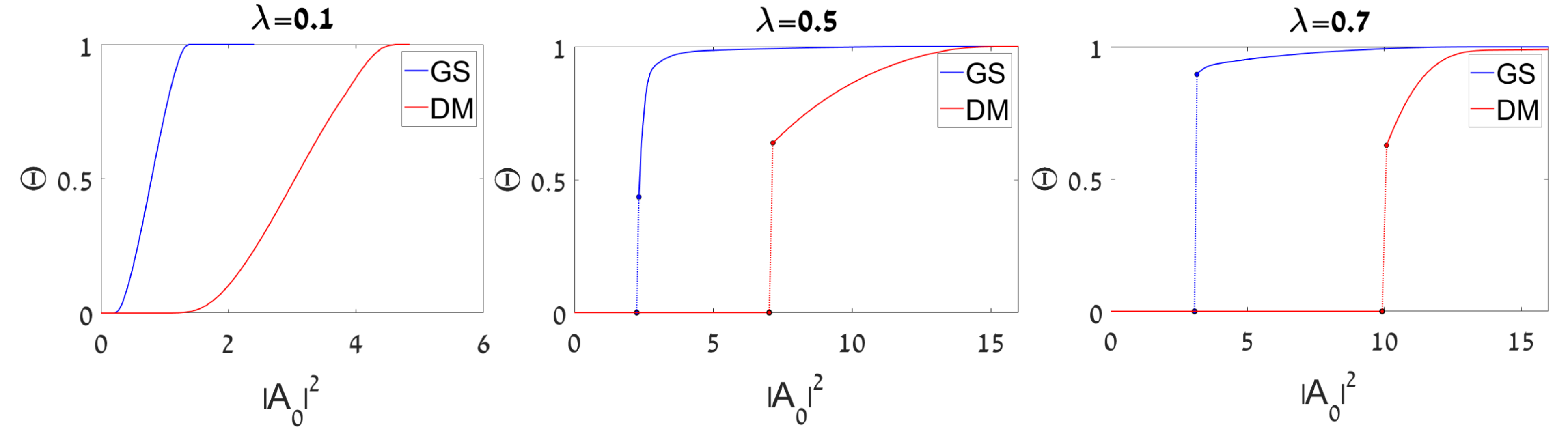
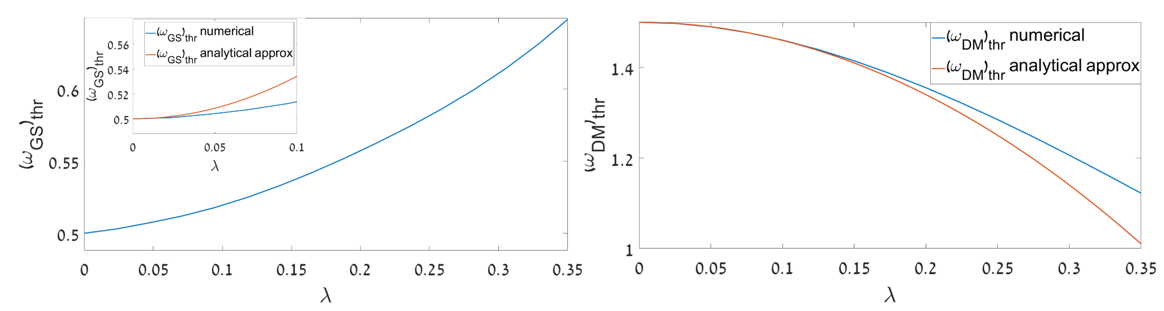
3.1.2. The Shift of the GS and DM Existence Thresholds at Small Values of Coupling Constant $\lambda$

At ${\mu }_{\mathrm{GS},\mathrm{DM}}^{\left(0\right)}<0$ the radiation is not generated by Equation (19), hence two-component bound states may exist in this case. Our next objective is to find, for the coupled system with $\lambda >0$, threshold values ${\left({\omega }_{\mathrm{GS},\mathrm{DM}}\right)}_{\mathrm{thr}}$ of the mismatch parameter $\omega$ in Equations (12) and (13), such that the bound states of the GS and DM types exist at

$$\omega >{\left({\omega }_{\mathrm{GS},\mathrm{DM}}\right)}_{\mathrm{thr}},$$

(21)

respectively. Obviously, ${\left({\omega }_{\mathrm{GS}}\right)}_{\mathrm{thr}}=1/2$ and ${\left({\omega }_{\mathrm{DM}}\right)}_{\mathrm{thr}}=3/2$ in the limit of $\lambda =0$, see Equation (17).

First, we aim to find lowest-order corrections to the GS and DM eigenvalues (17) for small $\lambda$. Then, a shift of the respective thresholds can be identified by setting ${\mu }_{\mathrm{GS},\mathrm{DM}}=0$. In the limit of $\lambda =0$, the GS and DM wave functions are taken as per Equations (14) and (15), respectively. With small $\lambda$, the first-order solution for $V\left(x\right)$, viz., $V\left(x\right)\equiv \lambda V_{\mathrm{GS},\mathrm{DM}}^{\left(1\right)}\left(x\right)$, must be found from the inhomogeneous equation, which follows from Equation (13), in which $\mu =0$ is set:

$$\frac{d^2}{d{x}^2}{V}_{\mathrm{GS},\mathrm{DM}}^{\left(1\right)}=-2U_{\mathrm{GS},\mathrm{DM}}^{\left(0\right)}\left(x\right).$$

(22)

Straightforward integration of Equation (22), with expressions (14) and (15) substituted on the right-hand side, yields

$$V_{\mathrm{GS}}^{\left(1\right)}\left(x\right)=-\sqrt{2}{\pi }^{1/4}\left[\frac{x}{\sqrt{2}}\mathrm{erf}\left(\frac{x}{\sqrt{2}}\right)+\sqrt{\frac{2}{\pi }}exp\left(-\frac{x^2}{2}\right)\right],$$

(23)

$$V_{\mathrm{DM}}^{\left(1\right)}\left(x\right)=2{\pi }^{1/4}\mathrm{erf}\left(\frac{x}{\sqrt{2}}\right),$$

(24)

where $\mathrm{erf}\left(x\right)$ is the standard error function, which is an odd function of x.

Next, the small perturbation in Equation (12), represented by term $\lambda V$, produces a small shift $\delta \mu$ of the eigenvalue, as a feedback from component V. According to the standard rule of quantum mechanics, which deals with the linear Schrödinger equation [66], in the first approximation of the perturbation theory, when $V\left(x\right)$ is replaced by expression (23) or (24), the result is

$$\delta {\mu }_{\mathrm{GS},\mathrm{DM}}=-{\lambda }^2{\int }_{-\infty }^{+\infty }{V}_{\mathrm{GS},\mathrm{DM}}^{\left(1\right)}\left(x\right)U_{\mathrm{GS},\mathrm{DM}}^{\left(0\right)}\left(x\right)dx\equiv -I_{\mathrm{GS},\mathrm{DM}}{\lambda }^2,$$

(25)

with coefficients

$$I_{\mathrm{GS}}=-3.414,I_{\mathrm{DM}}=4,$$

(26)

where the former and latter ones are computed, respectively, in a numerical form and analytically (note opposite signs of these coefficients). Then, the accordingly shifted threshold values sought for are

$${\left({\omega }_{\mathrm{GS}}\right)}_{\mathrm{thr}}=1/2-I_{\mathrm{GS}}{\lambda }^2,{\left({\omega }_{\mathrm{DM}}\right)}_{\mathrm{thr}}=3/2-I_{\mathrm{DM}}{\lambda }^2.$$

(27)

The analytical predictions are compared to numerical results, obtained from a solution of the linearized variant of Equations (12) and (13), in Figure 8. Note that the linear u-v coupling facilitates the formation of the DM bound state, by lowering ${\left({\omega }_{\mathrm{DM}}\right)}_{\mathrm{thr}}$, but impedes to form the GS, by making the respective threshold, ${\left({\omega }_{\mathrm{DM}}\right)}_{\mathrm{thr}}$, higher. It is seen that for the DM the analytical approximation is essentially more accurate than for the GS.

An example of a bound-state solution of linearized Equations (12) and (13) of the DM type, numerically found at $\lambda =0.225$ and $\omega =1.4$, i.e., below the threshold value ${\left({\omega }_{\mathrm{DM}}\right)}_{\mathrm{thr}}=1.5$, corresponding to the limit of $\lambda \to 0$, is displayed in Figure 9. The existence of the DM at this point agrees with the right panel of Figure 8.

3.1.3. The Analysis for Large Values of $\lambda$

In the opposite limit of large coupling constant $\lambda$, an analytical approximation for the discrete eigenvalues can be developed too. In this case, $\left|\mu \right|$ may also be large, ∼$\lambda$. In the zero-order approximation, one may neglect the derivative term in Equation (13), to obtain $V\approx -\left(\lambda /\mu \right)U$. Then, substituting this relation back into the originally neglected derivative term, one obtains a necessary correction to this relation:

$$V\approx -\frac{\lambda }{\mu }U+\frac{\lambda }{2{\mu }^2}\frac{d^{2}U}{d{x}^2}.$$

(28)

The subsequent substitution of this expression in the linearized Equation (12) leads to an equation for U which is tantamount to the usual stationary linear Schrödinger equation with the HO potential:

$$\left(\mu -\frac{{\lambda }^2}{\mu }+\omega \right)U+\frac{1}{2}\left(1+\frac{{\lambda }^2}{{\mu }^2}\right)\frac{d^{2}U}{d{x}^2}-\frac{1}{2}{x}^{2}U=0.$$

(29)

Then, the standard solution for the quantum-mechanical HO yields an equation which determines the spectrum of the eigenvalues:

$$\mu -\frac{{\lambda }^2}{\mu }+\omega =\left(\frac{1}{2}+n\right)\sqrt{1+\frac{{\lambda }^2}{{\mu }^2}},$$

(30)

where $n=0,1,2,\cdots$ is the quantum number. Taking into regard that $\lambda$ is now a large parameter, Equation (30) produces a final result for the spectrum,

$$\mu \approx -\lambda -\frac{\omega }{2}+\frac{1}{\sqrt{2}}\left(\frac{1}{2}+n\right).$$

(31)

The spectrum remains equidistant in the current approximation, while further corrections ∼$1/\lambda$ give rise to terms ∼${\left(1/2+n\right)}^2$, which break this property. As concerns the existence threshold for the bound states, Equation (31) predicts ${\omega }_{\mathrm{thr}}\approx -2\lambda$. The coefficient in this relation is not accurate, as the derivation is not valid for small $\left|\mu \right|$, but the implication is that, for large $\lambda$, ${\omega }_{\mathrm{thr}}$ drops to negative values with a large modulus, ∼$-\lambda$.

The prediction of the GS and DM eigenvalues, given by Equation (31) with $n=0$ and $n=1$, respectively, is compared to numerically found counterparts in Figure 10, which shows proximity between the analytical and numerical results. The plots do not terminate in the displayed domain, i.e., they do not reach the existence boundary.

3.1.4. Exact Solutions for One- and Two-Dimensional Bound States in the Continuum (BIC) in the Linear System

A remarkable property of the coupled half-trapped system, represented by the linearized version of Equations (10), (12) and (13), is that it admits particular spatially confined solutions in an exact analytical form. These are exceptional solutions, which, for an arbitrary value of the linear-coupling constant, $\lambda$, exist at a single, specially selected, value of the mismatch parameter, $\omega$, and with a single value of the eigenvalue, $\mu$. First, it is possible to find an exact mode which is a fundamental one (GS) in the V component, and a second-order mode in U:

$$\begin{array}{c}U\left(x\right)=U_0\left[\left({\lambda }^2-\frac{1}{2}\right)+x^2\right]exp\left(-\frac{x^2}{2}\right),\\ V\left(x\right)=-2\lambda U_{0}exp\left(-\frac{x^2}{2}\right),\\ U_0^2={\pi }^{-1/2}{\left({\lambda }^4+4{\lambda }^2+1/2\right)}^{-1},\\ \omega =\frac{9}{4}-\frac{{\lambda }^2}{2},\mu =\frac{1}{2}\left({\lambda }^2+\frac{1}{2}\right),\end{array}$$

(32)

with amplitude $U_0$ defined by condition $P=1$, see Equation (16). We stress that, as seen in Equation (32), this exact solution may only have $\mu >0$, i.e., it is BIC (a bound state in the continuous spectrum [58,59,60]), alias an embedded mode [61]. It is worthy to note that this BIC mode and additional ones, presented below, are found in the coupled system, with one component trapped in the HO potential.

In addition to the above spatially even solution, an odd one of the BIC type is available too. It is composed of a DM in the V component and a third-order mode in U. In the normalized form, i.e., with $P=1$ (as per Equation (16)), the solution is

$$\begin{array}{c}U\left(x\right)=U_{0}x\left[\left({\lambda }^2-\frac{3}{2}\right)+x^2\right]exp\left(-\frac{x^2}{2}\right),\\ V\left(x\right)=-2\lambda U_{0}xexp\left(-\frac{x^2}{2}\right),\\ U_0^2=2{\pi }^{-1/2}{\left({\lambda }^4+4{\lambda }^2+3/2\right)}^{-1},\\ \omega =\frac{11}{4}-\frac{{\lambda }^2}{2},\mu =\frac{1}{2}\left({\lambda }^2+\frac{3}{2}\right),\end{array}$$

(33)

which also exists at a single value of $\omega$, and with a single eigenvalue, $\mu >0$. Note that both exact solutions, given by Equations (32) and (33), may exists at positive and negative values of $\omega$, as well as at $\omega =0$ (in Equations (32) and (33), $\omega =0$ at ${\lambda }^2=9/2$ and ${\lambda }^2=11/2$, respectively).

These exact solutions for BIC states in the two-component systems are somewhat similar to those found in Ref. [67], which addressed a system of spin-orbit-coupled linear Gross–Pitaevskii equations for a binary BEC. In that work, exact solutions were produced for a specially designed form of the trapping potential.

The exact solutions of the linearized system may be tried as inputs in simulations of the full nonlinear system based on Equation (10), with $\omega$ selected as per the solutions. The simulations, performed with moderate values of the initial amplitude, produce a robust state with steady internal oscillations, as shown in Figure 11 for the attractive ($\sigma =1$) and repulsive ($\sigma =-1$) SPM nonlinearity. In addition, the simulations demonstrate weak emission of radiation in the untrapped (v) component. In the case of the self-attraction (the left panel in Figure 7), the radiation is almost invisible. The self-repulsion in the v component, naturally, enhances the emission, which becomes visible in the right panel of the figure. Still larger amplitudes of the input lead to irregular oscillations and conspicuous emission of radiation (not shown here in detail).

It may happen that the linearized system of Equations (12) and (13) produces isolated BIC/embedded modes in a numerical form at other values of parameters. The present work does not aim to carry our comprehensive search for such solutions. On the other hand, it is relevant to mention that a straightforward two-dimensional (2D) extension of the present system readily produces exceptional exact solutions for BIC/embedded modes of both fundamental (GS, alias zero-vorticity) and vortex types.

The 2D extension of the linearized form of Equation (10) is

$$\begin{array}{ccc}\hfill i{u}_z+\frac{1}{2}\left(u_{xx}+u_{yy}\right)+\lambda v-\frac{1}{2}\left(x^2+y^2\right)u& =& -\omega u,\hfill \\ & & \hfill \\ \hfill i{v}_z+\frac{1}{2}\left(v_{xx}+v_{yy}\right)+\lambda u& =& 0.\hfill \end{array}$$

(34)

Although the realization of this model in optics in not straightforward, it may be implemented for matter waves in a dual-core “pancake-shaped” holder of BEC [35,68]. In polar coordinates $\left(r,\theta \right)$, particular exact solutions of linear Equation (34), with all integer values of the vorticity, $S=0,1,2,\cdots$, are found as

$$\begin{array}{c}u=U_0{r}^S\left[\left({\lambda }^2-1-S\right)+r^2\right]exp\left(-i\mu z+iS\theta -\frac{r^2}{2}\right),\\ v=-2\lambda U_0{r}^{S}exp\left(-i\mu z+iS\theta -\frac{r^2}{2}\right),\\ \omega =\frac{1}{2}\left(5+S-{\lambda }^2\right),\mu =\frac{1}{2}\left({\lambda }^2+1+S\right),\end{array}$$

(35)

with arbitrary amplitude $U_0$ (the 2D solution of the GS type corresponds to $S=0$ in Equation (35)). As well as in 1D solutions (32) and (33), $\mu$ takes only positive values in the 2D solution, hence it also represents states of the BIC/embedded type.

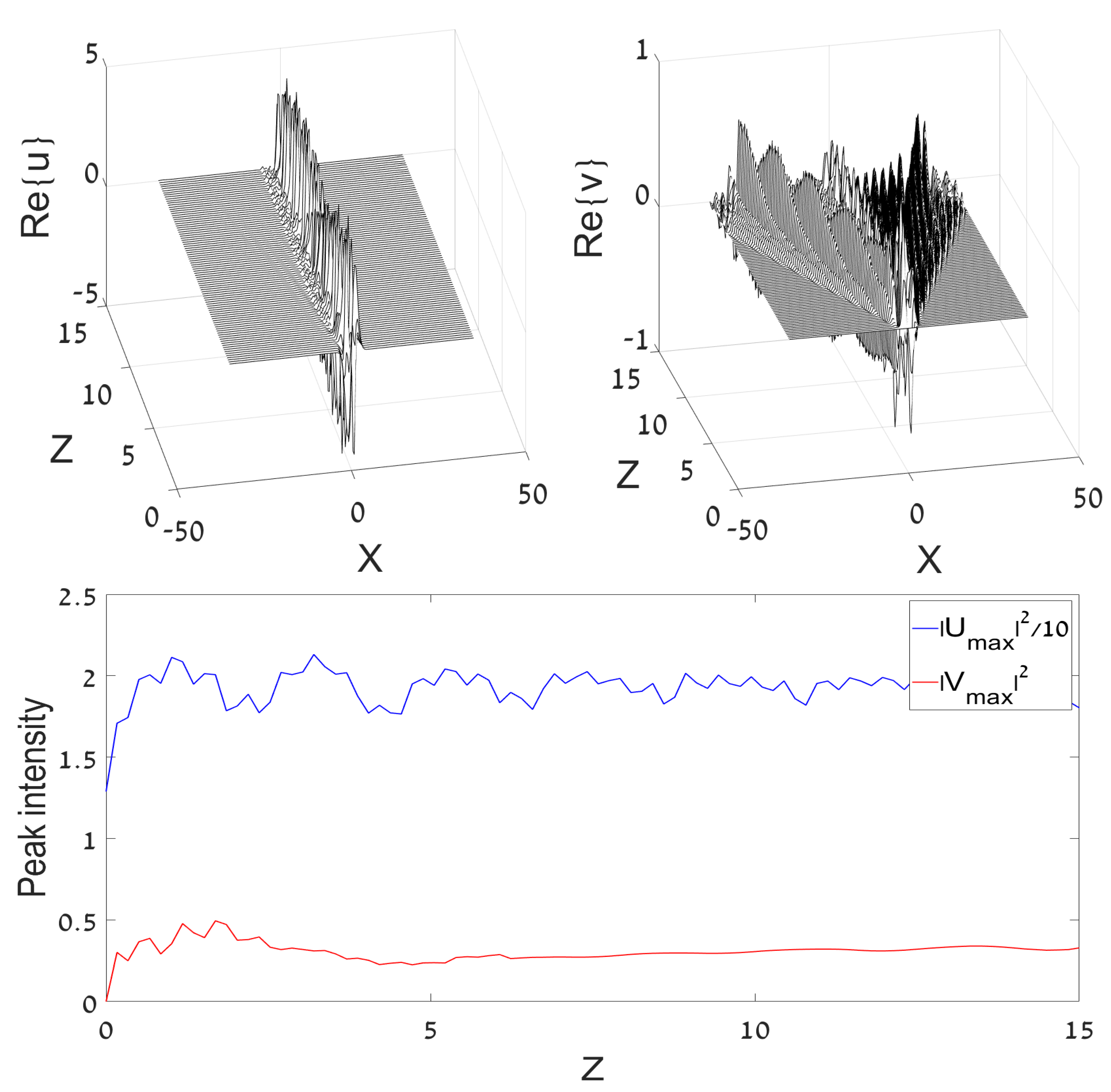
3.2. The Nonlinear Half-Trapped System

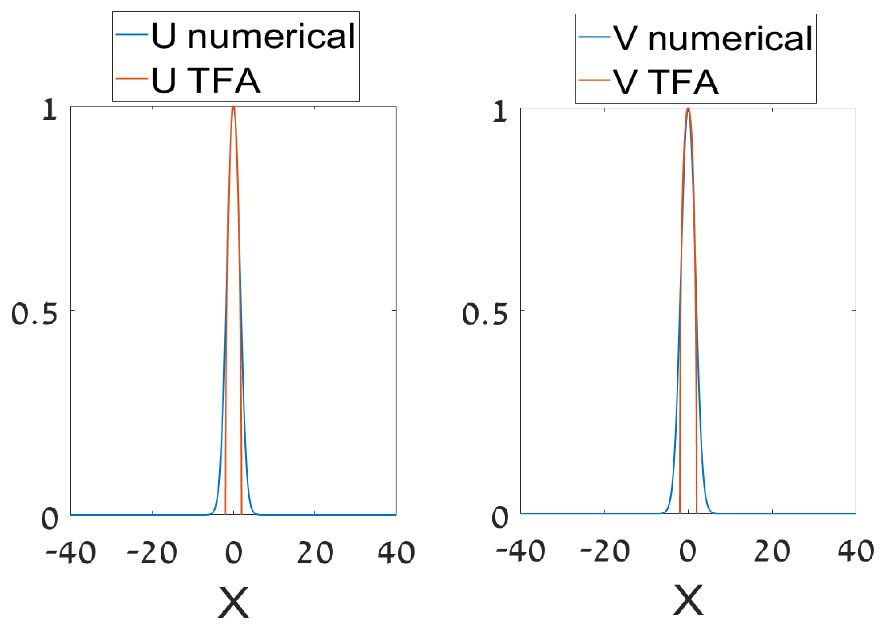
3.2.1. The Thomas–Fermi Approximation (TFA)

In the presence of the self-defocusing nonlinearity, $\sigma =-1$ in Equations (12) and (13), it is relevant to apply TFA to finding the GS of the half-trapped system, omitting the second derivatives in both equations [2], and keeping condition $\mu <0$, which is necessary for the existence of a generic (non-BIC) localized state in the V component. Then, Equation (13) with $g=0$ (the XPM coupling is omitted here) is solved as

$$U=\left(V/\lambda \right)\left(V^2-\mu \right),$$

(36)

and Equation (12) amounts to an algebraic equation for the squared amplitude $W\equiv -V^2/$$\mu >0$, viz.,

$$mW{\left(W+1\right)}^3+{\xi }^{2}W={\xi }_0^2-{\xi }^2,$$

(37)

where

$$\begin{array}{ccc}\hfill m& \equiv & -\frac{2\mu }{{\lambda }^2}>0,\xi \equiv -\frac{x}{\mu },\hfill \end{array}$$

(38)

$$\begin{array}{ccc}\hfill {\xi }_0^2& \equiv & -\frac{2}{{\mu }^3}\left[{\lambda }^2-\mu \left(\omega +\mu \right)\right],\hfill \end{array}$$

(39)

and the applicability condition for TFA is easily shown to be $m\ll 1$. The TFA solution exists under condition ${\xi }_0^2>0$ (see Equation (39)), i.e., in a finite interval (bandgap) of values of the propagation constant,

$$0<-\mu <\sqrt{{\lambda }^2+{\omega }^2/4}+\omega /2\equiv -{\mu }_0.$$

(40)

Outside of the bandgap, i.e., at $\mu <$${\mu }_0<0$, the TFA solution does not exist. In the bandgap, Equation (37) produces a usual GS profile, with a single value of W corresponding to each ${\xi }^2$ from region ${\xi }^2<{\xi }_0^2$ (see Figure 12, which displays a typical example of the TFA-predicted GS and its comparison with the numerically found counterpart). The solution vanishes at the border points, $\xi =\pm {\xi }_0$, and is equal to zero at ${\xi }^2>{\xi }_0^2$, so that the derivative of the TFA solution, $dW/d\xi$, is discontinuous at the border points, which is a usual peculiarity of the TFA [2,69].

Note that in the limit of large $\lambda$, the bandgap’s width, as given by Equation (40), is $-{\mu }_0\approx \lambda +\omega /2$, which is close to the largest value of $-\mu$ predicted by Equation (31) for the GS ($n=0$) in the linearized half-trapped system. Finally, the TFA solution may be cast in a simple explicit form close to the edge of the bandgap, i.e., at

$$\begin{array}{ccc}\hfill 0& <& \delta \mu \equiv \mu -{\mu }_0\ll -{\mu }_0,\hfill \end{array}$$

(41)

$$\begin{array}{ccc}\hfill {\xi }_0^2& \approx & -\left(4/{\mu }_0^3\right)\sqrt{{\lambda }^2+{\omega }^2/4}\delta \mu \hfill \end{array}$$

(42)

In this case, Equations (37) and (36) simplify to

$$U^2\approx \left\{\begin{array}{c}\left({\mu }_0^2/2\right)\left({\xi }_0^2-{\xi }^2\right),\mathrm{at}{\xi }^2<{\xi }_0^2,\\ 0\mathrm{at}{\xi }^2>{\xi }_0^2,\end{array}\right.$$

(43)

$$V^2\approx \left\{\begin{array}{c}\left({\lambda }^2/2\right)\left({\xi }_0^2-{\xi }^2\right),\mathrm{at}{\xi }^2<{\xi }_0^2,\\ 0\mathrm{at}{\xi }^2>{\xi }_0^2.\end{array}\right.$$

(44)

Expressions (42)–(44) make it possible to calculate the total power of the GS (see Equation (2)),

$$P\approx \frac{16}{3}\left({\lambda }^2+{\mu }_0^2\right){\left({\lambda }^2+\frac{{\omega }^2}{4}\right)}^{3/4}{\left(-{\mu }_0\right)}^{-7/2}{\left(\delta \mu \right)}^{3/2}.$$

(45)

Note that relation (45) satisfies the anti-Vakhitov–Kolokolov criterion, $dP/d\left(\delta \mu \right)>0$, which is a necessary condition for stability of localized states supported by self-repulsive nonlinearity [70], as is the case in the present setting (the Vakhitov–Kolokolov criterion proper, $dP/d\left(\delta \mu \right)<0$, is a well-known necessary condition for stability of states in models with self-attraction [71,72,73]).

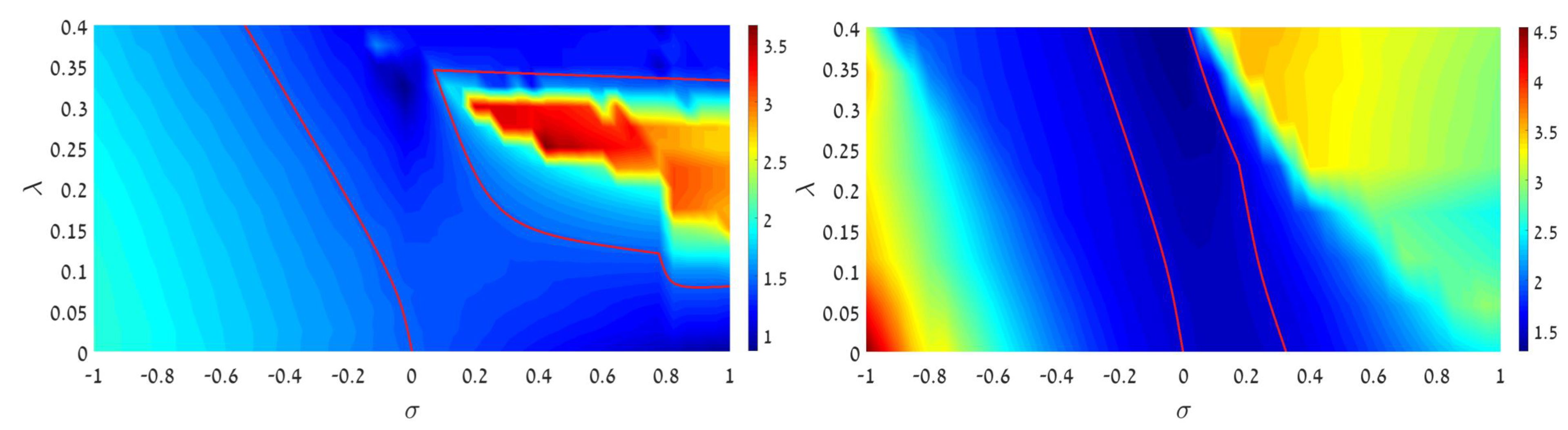
3.2.2. Existence Boundaries for Nonlinear States

The shrinkage of the existence region for GS solutions, and its expansion for DM ones, in the linear version of the coupled half-trapped system, shown in Figure 8, suggests identifying existence boundaries of the same states in the full nonlinear system. Numerical data, necessary for the delineation of the existence region of the GSs and DMs in the nonlinear system, were collected by solving Equations (12) and (13) for spatially even and odd modes with the fixed total power, $P=1$ (as per Equation (16)), while the linear-coupling coefficient, $\lambda$, and the nonlinearity coefficient, $\sigma$, were varied, the latter one taking both positive and negative values (for the self-attraction/repulsion). The results are summarized by the heatmap in Figure 13 (for the GS) and Figure 14 (for the DM), which show threshold values of the mismatch parameter, defined as per Equation (21).

Nontrivial parametric areas for the GS and DM solutions are identified as domains with, respectively, ${\left({\omega }_{\mathrm{GS}}\right)}_{\mathrm{thr}}<1/2$ and ${\left({\omega }_{\mathrm{DM}}\right)}_{\mathrm{thr}}<3/2$. The former one is surrounded by red lines in Figure 13, and its counterpart for the DMs is located between red lines in Figure 14. In these areas, the coupled half-trapped system maintains stable localized GSs at $\omega <1/2$, and DMs at $\omega <3/2$, while in the absence of the coupling they may only exist at $\omega >1/2$ and $\omega >3/2$, respectively.

Note that the vertical cross-section of the heatmap in Figure 13, drawn through $\sigma =0$ (along which the system remains linear), that starts from $\lambda =0$, belongs to the area with ${\left({\omega }_{\mathrm{GS}}\right)}_{\mathrm{thr}}>1/2$, in agreement with the result for the linear system, which shows that the coupling impedes the existence of the GS, see the left panel of Figure 8 and Equation (27). Furthermore, Figure 13 demonstrates that the SPM nonlinearity of either sign facilitates the creation of GS in parameter regions surrounded by red lines. Naturally, the self-attraction ($\sigma >0$) helps to create such states starting from arbitrarily small values of $\lambda$, while the self-repulsion ($\sigma <0$) can do it in the region separated by a gap from $\lambda =0$. Nevertheless, at $\lambda >0.24$ the detrimental effect of the linear coupling cannot be outweighed by the SPM nonlinearity.

In Figure 14, the vertical cross-section corresponding to the linear system ($\sigma =0$) entirely belongs to the nontrivial area, with ${\left({\omega }_{\mathrm{DM}}\right)}_{\mathrm{thr}}<3/2$, also in agreement with Equation (27) and the right panel of Figure 8. Figure 14 demonstrates that the nonlinearity, generally, impedes the maintenance of the localized DMs. This conclusion is supported, in particular, by the comparison of panels (a) and (b) in the figure, which shows that the addition of the attractive XPM nonlinearity with the SPM conspicuously reduces the remaining nontrivial area.

4. Conclusions

The objective of this work is to analyze new effects in the symmetric and asymmetric systems of linearly coupled fields, which are subject to the action of the HO (harmonic-oscillator) trapping potential and cubic self-attraction or repulsion. The system can be implemented in nonlinear optics and BEC. In the symmetric system, with identical HO potentials applied to both components, we focus on the consideration of JO (Josephson oscillations) in the system, by launching, in one component, an input in the form of the GS (ground state) or DM (dipole mode) of the HO potential. On the basis of systematically collected numerical data, we have identified two transitions in the system’s dynamics, which occur with the increase of the input’s power in the case of the self-attraction. The first is SSB (spontaneous symmetry breaking) between the linearly coupled components in the dynamical JO state. At a higher power, the nonlinearity causes a transition from regular JO, initiated by the GS input, to chaotic dynamics. This transition is identified through consideration of spectral characteristics of the dynamical regime. The input in the form of the DM undergoes the chaotization at essentially smaller powers than the dynamical regime initiated by the GS input, which is followed by the SSB at slightly higher powers. In the case of self-repulsion, SSB does not occur, while the chaotization takes place in a weak form, in a small part of the parameter space.

In the half-trapped system, with the HO potential acting on a single component, a nontrivial issue is identification of the system’s linear spectrum, i.e., a parameter region in which the linearized system maintains trapped binary (two-component) modes. This problem is solved here analytically in the limit cases of weak and strong linear coupling, and in the numerical form in the general case. In particular, the linear coupling between the components leads to the shrinkage of the spectral band in which the GS exists, and expansion of the existence band for the DM. The existence region for trapped states in the full nonlinear system is identified numerically, and such states are constructed analytically by means of the TFA (Thomas–Fermi approximation). In addition, exceptional solutions of the linearized system of the BIC (bound-state-in-continuum), alias embedded, type were found in the exact analytical form, in both the 1D and 2D settings, the 2D solution being found with an arbitrary value of the vorticity.

The work may be extended by considering inputs in the form of higher-order HO eigenstates. Another relevant direction for the extension of the analysis is a systematic study of the 2D system.

References

1. Pethick, C.J.; Smith, H. Bose-Einstein Condensation in Dilute Gases; Cambridge University Press: Cambridge, UK, 2002. [Google Scholar]
2. Pitaevskii, L.P.; Stringari, S. Bose-Einstein Condensation; Oxford University Press: Oxford, UK, 2003. [Google Scholar]
3. Kevrekidis, P.G.; Frantzeskakis, D.J.; Carretero-Gonz ález, R. Emergent Nonlinear Phenomena in Bose-Einstein Condensates: Theory and Experiment; Springer: Heidelberg, Germany, 2008. [Google Scholar]
4. Schneider, B.I.; Feder, D.L. Numerical approach to the ground and excited states of a Bose-Einstein condensed gas confined in a completely anisotropic trap. Phys. Rev. A 1999, 59, 2232–2242. [Google Scholar] [CrossRef] [Green Version]
5. Adhikari, S.K. Numerical solution of the two-dimensional Gross-Pitaevskii equation for trapped interacting atoms. Phys. Lett. A 2000, 265, 91–96. [Google Scholar] [CrossRef] [Green Version]
6. Busch, T.; Anglin, J.R. Motion of dark solitons in trapped Bose-Einstein condensates. Phys. Rev. Lett. 2000, 84, 2298–2301. [Google Scholar] [CrossRef] [Green Version]
7. Kivshar, Y.S.; Alexander, T.J.; Turitsyn, S.K. Nonlinear modes of a macroscopic quantum oscillator. Phys. Lett. 2001, 278, 225–230. [Google Scholar] [CrossRef] [Green Version]
8. Alexander, T.J.; Bergé, L. Ground states and vortices of matter-wave condensates and optical guided waves. Phys. Rev. E 2002, 65, 026611. [Google Scholar] [CrossRef] [Green Version]
9. Huang, G.; Szeftel, J.; Zhu, S. Dynamics of dark solitons in quasi-one-dimensional Bose-Einstein condensates. Phys. Rev. A 2002, 65, 053605. [Google Scholar] [CrossRef]
10. Parker, N.G.; Proukakis, N.P.; Leadbeater, M.; Adams, C.S. Soliton-sound interactions in quasi-one-dimensional Bose-Einstein condensates. Phys. Rev. Lett. 2003, 90, 220401. [Google Scholar] [CrossRef]
11. Pelinovsky, D.E.; Frantzeskakis, D.J.; Kevrekidis, P.G. Oscillations of dark solitons in trapped Bose-Einstein condensates. Phys. Rev. E 2005, 72, 016615. [Google Scholar] [CrossRef] [Green Version]
12. Brazhnyi, V.A.; Konotop, V.V. Stable and unstable vector dark solitons of coupled nonlinear Schrödinger equations: Application to two-component Bose-Einstein condensates. Phys. Rev. E 2005, 72, 026616. [Google Scholar] [CrossRef] [Green Version]
13. Parker, N.G.; Proukakis, N.G.; Adams, C.S. Dark soliton decay due to trap anharmonicity in atomic Bose-Einstein condensates. Phys. Rev. A 2010, 81, 033606. [Google Scholar] [CrossRef] [Green Version]
14. Bland, T.; Parker, N.G.; Proukakis, N.P.; Malomed, B.A. Probing quasi-integrability of the Gross-Pitaevskii equation in a harmonic-oscillator potential. J. Phys. B Atomic Mol. Opt. Phys. 2018, 51, 205303. [Google Scholar] [CrossRef] [Green Version]
15. Raghavan, S.; Agrawal, G.P. Spatiotemporal solitons in inhomogeneous nonlinear media. Opt. Commun. 2000, 180, 377–382. [Google Scholar] [CrossRef]
16. Zezyulin, D.A.; Alfimov, G.L.; Konotop, V.V. Nonlinear modes in a complex parabolic potential. Phys. Rev. A 2010, 81, 013606. [Google Scholar] [CrossRef]
17. Charalampidis, E.G.; Kevrekidis, P.G.; Frantzeskakis, D.J.; Malomed, B.A. Dark-bright solitons in coupled NLS equations with unequal dispersion coefficients. Phys. Rev. E 2015, 91, 012924. [Google Scholar] [CrossRef] [Green Version]
18. Mayteevarunyoo, T.; Malomed, B.A.; Skryabin, D.V. One- and two-dimensional modes in the complex Ginzburg-Landau equation with a trapping potential. Opt. Exp. 2018, 26, 8849–8865. [Google Scholar] [CrossRef] [Green Version]
19. Leib, M.; Deppe, F.; Marx, A.; Gross, R.; Hartmann, M.J. Networks of nonlinear superconducting transmission line resonators. New J. Phys. 2012, 14, 075024. [Google Scholar] [CrossRef] [Green Version]
20. Kivshar, Y.S.; Agrawal, G.P. Optical Solitons: From Fibers to Photonic Crystals; Academic Press: San Diego, CA, USA, 2003. [Google Scholar]
21. Morsch, O.; Oberthaler, M. Dynamics of Bose-Einstein condensates in optical lattices. Rev. Modern Phys. 2006, 78, 179–215. [Google Scholar] [CrossRef]
22. Joannopoulos, J.D.; Johnson, S.G.; Winn, J.N.; Meade, R.D. Photonic Crystals: Molding the Flow of Light; Princeton University Press: Princeton, NJ, USA, 2008. [Google Scholar]
23. Skorobogatiy, M.; Yang, J. Fundamentals of Photonic Crystal Guiding; Cambridge University Press: Cambridge, UK, 2008. [Google Scholar]
24. Cerda-Mendez, E.A.; Sarkar, D.; Krizhanovskii, D.N.; Gavrilov, S.S.; Biermann, K.; Skolnick, M.S.; Santos, P.V. Exciton-polariton gap solitons in two-dimensional lattices. Phys. Rev. Lett. 2013, 111, 146401. [Google Scholar] [CrossRef]
25. Brazhnyi, V.A.; Konotop, V.V. Theory of nonlinear matter waves in optical lattices. Modern Phys. Lett. B 2004, 18, 627–651. [Google Scholar] [CrossRef] [Green Version]
26. Sakaguchi, H.; Malomed, B.A. Dynamics of positive- and negative-mass solitons in optical lattices and inverted traps. J. Phys. B 2004, 37, 1443–1459. [Google Scholar] [CrossRef] [Green Version]
27. Zakharov, V.E.; Manakov, S.V.; Novikov, S.P.; Pitaevskii, L.P. Theory of Solitons: Inverse Scattering Method; English translation: Consultants Bureau, New York, 1984; Nauka: Moscow, Russia, 1980. [Google Scholar]
28. Zakharov, V.; Dias, F.; Pushkarev, A. One-dimensional wave turbulence. Phys. Rep. 2004, 398, 1–65. [Google Scholar] [CrossRef]
29. Mazets, I.E.; Schmiedmayer, J. Thermalization in a quasi-one-dimensional ultracold bosonic gas. New J. Phys. 2010, 12, 055023. [Google Scholar] [CrossRef]
30. Cockburn, S.P.; Negretti, A.; Proukakis, N.P.; Henkel, C. Comparison between microscopic methods for finite-temperature Bose gases. Phys. Rev. A 2011, 83, 043619. [Google Scholar] [CrossRef] [Green Version]
31. Grisins, P.; Mazets, I.E. Thermalization in a one-dimensional integrable system. Phys. Rev. A 2011, 84, 053635. [Google Scholar] [CrossRef] [Green Version]
32. Thomas, K.F.; Davis, M.J.; Kheruntsyan, K.V. Thermalization of a quantum Newton’s cradle in a one-dimensional quasicondensate. Phys. Rev. A 2021, 103, 023315. [Google Scholar] [CrossRef]
33. Merhasin, M.I.; Malomed, B.A.; Driben, R. Transition to miscibility in a binary Bose-Einstein condensate induced by linear coupling. J. Phys. B 2005, 38, 877–892. [Google Scholar] [CrossRef]
34. Nistazakis, H.E.; Frantzeskakis, D.J.; Kevrekidis, P.G.; Malomed, B.A.; Carretero-Gonzalez, R. Bright-dark soliton complexes in spinor Bose-Einstein condensates. Phys. Rev. A 2008, 77, 033612. [Google Scholar] [CrossRef] [Green Version]
35. Chen, Z.; Li, Y.; Malomed, B.A.; Salasnich, L. Spontaneous symmetry breaking of fundamental states, vortices, and dipoles in two and one-dimensional linearly coupled traps with cubic self-attraction. Phys. Rev. A 2016, 96, 033621. [Google Scholar] [CrossRef] [Green Version]
36. Decker, M.; Ruther, M.; Kriegler, C.E.; Zhou, J.; Soukoulis, C.M.; Linden, S.; Wegener, M. Strong optical activity from twisted-cross photonic metamaterials. Opt. Lett. 2009, 34, 2501–2503. [Google Scholar] [CrossRef] [PubMed]
37. Ballagh, R.J.; Burnett, K.; Scott, T.F. Theory of an output coupler for Bose-Einstein condensed atoms. Phys. Rev. Lett. 1997, 78, 1607–1611. [Google Scholar] [CrossRef]
38. Öhberg, P.; Stenholm, S. Internal Josephson effect in trapped double condensates. Phys. Rev. A 1999, 59, 3890–3895. [Google Scholar] [CrossRef]
39. Son, D.T.; Stephanov, M.A. Domain walls of relative phase in two-component Bose-Einstein condensates. Phys. Rev. A 2002, 65, 063621. [Google Scholar] [CrossRef] [Green Version]
40. Jenkins, S.D.; Kennedy, T.A.B. Dynamic stability of dressed condensate mixtures. Phys. Rev. A 2003, 68, 053607. [Google Scholar] [CrossRef]
41. Malomed, B.A. (Ed.) Spontaneous Symmetry Breaking, Self-Trapping, and Josephson Oscillations; Springer: Berlin/Heidelberg, Germany, 2013. [Google Scholar]
42. Hung, N.V.; Tai, L.X.T.; Bugar, I.; Longobucco, M.; Buzcy ński, R.; Malomed, B.A.; Trippenbach, M. Reversible ultrafast soliton switching in dual-core highly nonlinear optical fibers. Opt. Lett. 2020, 45, 5221–5224. [Google Scholar]
43. Mineev, V.P. The theory of the solution of two near-ideal Bose gases. Zh. Eksp. Teor. Fiz. 1974, 67, 263–272, [English translation: Sov. Phys. JETP 1974, 40, 132–136]. [Google Scholar]
44. Malomed, B.A. Solitons and nonlinear dynamics in dual-core optical fibers. In Handbook of Optical Fibers; Peng, G.-D., Ed.; Springer: Berlin/Heidelberg, Germany, 2018; pp. 421–474. [Google Scholar]
45. Tratnik, M.V.; Sipe, J.E. Bound solitary waves in a birefringent optical fiber. Phys. Rev. A 1988, 38, 2011–2017. [Google Scholar] [CrossRef]
46. Paré, C.; Orjańczyk, M.F. Approximate model of soliton dynamics in all-optical couplers. Phys. Rev. A 1990, 41, 6287. [Google Scholar] [CrossRef]
47. Maimistov, A.I. Propagation of a light pulse in nonlinear tunnel-coupled optical waveguides. Kvant. Elektron. 1991, 18, 758, [English translation: Sov. J. Quantum Electron. 1991, 21, 687].. [Google Scholar] [CrossRef]
48. Uzunov, I.M.; Muschall, R.; Goelles, M.; Kivshar, Y.S.; Malomed, B.A.; Lederer, F. Pulse switching in nonlinear fiber directional couplers. Phys. Rev. E 1995, 51, 2527–2536. [Google Scholar] [CrossRef]
49. Abbarchi, M.; Amo, A.; Sala, V.G.; Solnyshkov, D.D.; Flayac, H.; Ferrier, L.; Sagnes, I.; Galopin, E.; Lemaître, A.; Malpuech, G.; et al. Macroscopic quantum self-trapping and Josephson oscillations of exciton polaritons. Nat. Phys. 2013, 9, 275. [Google Scholar] [CrossRef]
50. Milburn, G.J.; Corney, J.; Wright, E.M.; Walls, D.F. Quantum dynamics of an atomic Bose-Einstein condensate in a double-well potential. Phys. Rev. A 1997, 55, 4318. [Google Scholar] [CrossRef] [Green Version]
51. Smerzi, A.; Fantoni, S.; Giovanazzi, S.; Shenoy, S.R. Quantum coherent atomic tunneling between two trapped Bose-Einstein condensates. Phys. Rev. Lett. 1997, 79, 4950. [Google Scholar] [CrossRef] [Green Version]
52. Albiez, M.; Gati, R.; Fölling, J.; Hunsmann, S.; Cristiani, M.; Oberthaler, M.K. Direct observation of tunneling and nonlinear self-trapping in a single bosonic Josephson junction. Phys. Rev. Lett. 2005, 95, 010402. [Google Scholar] [CrossRef] [PubMed] [Green Version]
53. Shin, Y.; Jo, G.-B.; Saba, M.; Pasquini, T.A.; Ketterle, W.; Pritchard, D.E. Optical weak link between two spatially separated Bose-Einstein condensates. Phys. Rev. Lett. 2005, 95, 170402. [Google Scholar] [CrossRef] [PubMed] [Green Version]
54. Levy, S.; Lahoud, E.; Shomroni, I.; Steinhauer, J. The a.c. and d.c. Josephson effects in a Bose–Einstein condensate. Nature 2007, 449, 579–583. [Google Scholar] [CrossRef]
55. Chen, Z.; Li, Y.; Malomed, B.A. Josephson oscillations of chirality and identity in two-dimensional solitons in spin-orbit-coupled condensates. Phys. Rev. Res. 2020, 2, 033214. [Google Scholar] [CrossRef]
56. Sakaguchi, H.; Malomed, B.A. Symmetry breaking in a two-component system with repulsive interactions and linear coupling. Comm. Nonlin. Sci. Num. Sim. 2020, 92, 105496. [Google Scholar] [CrossRef]
57. Panoiu, N.-C.; Malomed, B.A.; Osgood, R.M., Jr. Semidiscrete solitons in arrayed waveguide structures with Kerr nonlinearity. Phys. Rev. A 2008, 78, 013801. [Google Scholar] [CrossRef] [Green Version]
58. Stillinger, F.H.; Herrick, D.R. Bound states in continuum. Phys. Rev. A 1975, 11, 446–454. [Google Scholar] [CrossRef]
59. Kodigala, A.; Lepetit, T.; Gu, Q.; Bahari, B.; Fainman, Y.; Kante, B. Lasing action from photonic bound states in continuum. Nature 2017, 54, 196–199. [Google Scholar] [CrossRef]
60. Midya, B.; Konotop, V.V. Coherent-perfect-absorber and laser for bound states in a continuum. Opt. Lett. 2018, 43, 607–610. [Google Scholar] [CrossRef]
61. Champneys, A.R.; Malomed, B.A.; Yang, J.; Kaup, D.J. “Embedded solitons”: Solitary waves in resonance with the linear spectrum. Physica D 2001, 152–153, 340–354. [Google Scholar] [CrossRef] [Green Version]
62. Ananikian, D.; Bergeman, T. Gross-Pitaevskii equation for Bose particles in a double-well potential: Two-mode models and beyond. Phys. Rev. A 2006, 73, 013604. [Google Scholar] [CrossRef] [Green Version]
63. Kartashov, Y.V.; Konotop, V.V.; Vysloukh, V.A. Dynamical suppression of tunneling and spin switching of a spin-orbit-coupled atom in a double-well trap. Phys. Rev. A 2018, 97, 063609. [Google Scholar] [CrossRef] [Green Version]
64. Kivshar, Y.S.; Malomed, B.A. Dynamics of solitons in nearly integrable systems. Rev. Mod. Phys. 1989, 61, 763–915. [Google Scholar] [CrossRef]
65. Iooss, G.; Joseph, D.D. Elementary Stability Bifurcation Theory; Springer: New York, NY, USA, 1980. [Google Scholar]
66. Landau, L.D.; Lifshitz, E.M. Quantum Mechanics; Nauka Publishers: Moscow, Russia, 1974. [Google Scholar]
67. Kartashov, Y.V.; Konotop, V.V.; Torner, L. Bound states in the continuum in spin-orbit-coupled atomic systems. Phys. Rev. A 2017, 96, 033619. [Google Scholar] [CrossRef] [Green Version]
68. dos Santos, M.C.P.; Malomed, B.A.; Cardoso, W.B. Double-layer Bose-Einstein condensates: A quantum phase transition in the transverse direction, and reduction to two dimensions. Phys. Rev. E 2020, 102, 042209. [Google Scholar] [CrossRef] [PubMed]
69. Fetter, A.L.; Feder, D.L. Beyond the Thomas-Fermi approximation for a trapped condensed Bose-Einstein gas. Phys. Rev. A 1998, 58, 3185–3194. [Google Scholar] [CrossRef] [Green Version]
70. Sakaguchi, H.; Malomed, B.A. Solitons in combined linear and nonlinear lattice potentials. Phys. Rev. A 2010, 81, 013624. [Google Scholar] [CrossRef] [Green Version]
71. Vakhitov, N.G.; Kolokolov, A.A. Stationary solutions of the wave equation in a medium with nonlinearity saturation. Radiophys. Quant. Electron. 1973, 16, 783–789. [Google Scholar] [CrossRef]
72. Bergé, L. Wave collapse in physics: Principles and applications to light and plasma waves. Phys. Rep. 1998, 303, 259–370. [Google Scholar] [CrossRef]
73. Fibich, G. The Nonlinear Schrödinger Equation: Singular Solutions and Optical Collapse; Springer: Heidelberg, Germany, 2015. [Google Scholar]
Figure 1. A typical example of a regular Josephson dynamical regime, initiated by the DM (dipole mode) input launched in the u component (as given by Equation (5) with z = 0 and A 0 = 1 ). The solution is produced by simulations of Equation (1) with λ = σ = Ω = 1 , g = 0 . Plots in the top row display the evolution of components u x , z and v x , z . Left bottom: The evolution of the peak intensities of both components, U max 2 ( z ) max x u ( x , z ) 2 and V max 2 ( z ) max x v ( x , z ) 2 . Right bottom: The power spectrum of oscillations of the two components, defined as per Equation (7). The spectra are virtually identical for both components.
Symmetry 13 00372 g001
Figure 2. The same as in Figure 1, but for a typical example of a chaotic dynamical regime, initiated by the DM input (5) with a larger amplitude, A 0 = 4 . Note different scales on vertical axes in two plots in the left panel.
Symmetry 13 00372 g002
Figure 3. Heatmaps of values of sharpness (8) of the central spectral peak quantifying proximity of the system’s dynamics to the regular regime. The maps are plotted in the plane of the linear-coupling strength, λ , and intensity of the input, A 0 2 , which is launched in one component. (Top left): The GS input, given by Equation (4) at z = 0 , in the case of the self-attraction ( σ = + 1 ). (Top right): The same, but in the case of self-repulsion ( σ = 1 ). (Bottom left): The same as in the top left panel, but produced by the DM input, given by Equation (5) at z = 0 . (Bottom right): The same as in the bottom left panel, but in the case of self-repulsion ( σ = 1 ). In all cases, g = 0 is set in Equation (1) (no XPM interaction between the components). Black curves cutting the left panels in their lower areas designate the onset of SSB (spontaneous symmetry breaking), signalized by appearance of θ 0 , see Equation (9).
Symmetry 13 00372 g003
Figure 4. Plots of the SSB (spontaneous symmetry breaking) in the dynamical states initiated by the GS (ground state) and DM (dipole mode) inputs: the asymmetry parameter, defined as per Equation (9), is plotted versus the intensity of the input, A 0 2 , for three different fixed values of the linear-coupling constant, λ , as indicated in the figure.
Symmetry 13 00372 g004
Figure 5. Simulations of the evolution of the linearized half-trapped system (10), displayed in the untrapped component by plotting Re v x , z . (Left): Emission of radiation generated by the GS (ground state) populating the trapped component, u x , z (see Equation (14)), with ω = 0.25 in Equation (10). (Right): The same, but for the radiation generated by the DM (dipole mode) in the trapped component (see Equation (15)), with ω = 0 . In both cases, the linear-coupling constant is λ = 0.05 .
Symmetry 13 00372 g005
Figure 6. (Left): The evolution of fields u and v in the half-trapped system, as produced by simulations of Equation (10) with ω = 0 and coupling constant λ = 1 , initiated by the DM input in the u core, taken as per Equation (14) with A 0 = 0.1 . Here and in Figure 7, spurious left-right asymmetry of the radiation field in the v component is an illusion produced by plotting. (Right): The evolution of the peak intensities of both components, max x u ( x , t ) 2 and max x v x , t 2 .
Symmetry 13 00372 g006
Figure 7. The same as in Figure 6, but for a large amplitude of the DM input in the u component, A 0 = 8 .
Symmetry 13 00372 g007
Figure 8. The analytically predicted and numerically found threshold values of the mismatch parameter, ω , above which the GS and DM solutions (the left and right panels, respectively) are produced, for the half-trapped system, by the linearized version of Equations (12) and (13), vs. coupling constant λ . The analytical results are produced by Equation (27). For the GS, they are shown (in the inset) only for relatively small values of λ , as in this case the analytical approximation is inaccurate at larger λ .
Symmetry 13 00372 g008
Figure 9. A bound state of the DM (dipole mode) type in the half-trapped system, found as a numerical solution of Equations (12) and (13) with ω = 1.4 , λ = 0.225 , and σ = 0 (the linearized version). The eigenvalue corresponding to this solution is μ 0.036 .
Symmetry 13 00372 g009
Figure 10. (The top row): left and right panels display the analytically predicted eigenvalues given by Equation (31) with n = 0 and n = 1 , for the ground state (GS) and dipole mode (DM), respectively, of the half-trapped system, and their counterparts produced by the numerical solution of linearized coupled Equations (12) and (13), as functions of the linear-coupling constant, λ , and mismatch parameter, ω . (The bottom row): cross sections of the respective top panels along the diagonal connecting points λ , ω = 0.10 and 10 , 0 . The results shown in these plots are relevant for relatively large values of λ .
Symmetry 13 00372 g010
Figure 11. The evolution initiated by the exceptional (BIC) exact solution (32) of the system of linearized Equations (12) and (13), as produced by simulations of the full nonlinear half-trapped system (10), with the attractive SPM, σ = 1 in the top row, and repulsive σ = 1 in the bottom one. Other parameters are g = 0 , λ = 7 / 2 and ω = 1 / 2 , which are related as per Equation (32).
Symmetry 13 00372 g011
Figure 12. A typical example of the GS solution predicted by TFA (Thomas–Fermi approximation) for the half-trapped system, as per Equations (36)–(39), for σ = 1 , g = 0 , λ = 8 , μ = 4 , and its comparison to the numerically found counterpart. The respective value of parameter m (see Equation (38)), which should be small for the applicability of TFA, is m = 0.125 .
Symmetry 13 00372 g012
Figure 13. The heatmap of threshold values of the mismatch parameter, ω GS thr , in the half-trapped system, based on Equations (12) and (13). For given values of the nonlinearity and linear-coupling coefficients, σ and λ , the stable GS (ground state), subject to the normalization condition P = 1 (see Equation (16)), exist above the threshold, i.e., at ω ω GS thr . Positive and negative values of σ correspond to the attractive and repulsive sign of the self-interaction, respectively. The nontrivial region is one confined by red lines, in which the result is ω GS thr < 1 / 2 , i.e., the nonlinearity and linear coupling help to maintain self-trapped GSs in the parameter area where the decoupled system, with λ = 0 , cannot create such states.
Symmetry 13 00372 g013
Figure 14. The same as in Figure 13, but for DMs (dipole modes), obtained as numerical solutions to Equations (12) and (13) with g = 0 and g = 1 (the left and right panels, respectively). In this case, the nontrivial region, located between the red boundaries, is one with ω DM thr < 3 / 2 .
Symmetry 13 00372 g014
Publisher’s Note: MDPI stays neutral with regard to jurisdictional claims in published maps and institutional affiliations.