Quantum Calculations on Ion Channels: Why Are They More Useful Than Classical Calculations, and for Which Processes Are They Essential?

Abstract

There are reasons to consider quantum calculations to be necessary for ion channels, for two types of reasons. The calculations must account for charge transfer, and the possible switching of hydrogen bonds, which are very difficult with classical force fields. Without understanding charge transfer and hydrogen bonding in detail, the channel cannot be understood. Thus, although classical approximations to the correct force fields are possible, they are unable to reproduce at least some details of the behavior of a system that has atomic scale. However, there is a second class of effects that is essentially quantum mechanical. There are two types of such phenomena: exchange and correlation energies, which have no classical analogues, and tunneling. Tunneling, an intrinsically quantum phenomenon, may well play a critical role in initiating a proton cascade critical to gating. As there is no classical analogue of tunneling, this cannot be approximated classically. Finally, there are energy terms, exchange and correlation energy, whose values can be approximated classically, but these approximations must be subsumed within classical terms, and as a result, will not have the correct dependence on interatomic distances. Charge transfer, and tunneling, require quantum calculations for ion channels. Some results of quantum calculations are shown.

1. Introduction

Ion channels are proteins that allow the passage of ions, especially Na⁺, K⁺, and Ca⁺⁺ across membranes. In this discussion, we will give most examples from a particular potassium channel. However, we will be primarily concerned with the question of the best means of obtaining information from calculations, which we will apply much more generally. In essence, there are two approaches to calculations on proteins, and channels in particular. The calculations can be done using classical or quantum physics, and we will argue that quantum physics is necessary. For one thing, there are certain quantum phenomena that are essentially impossible to simulate using classical physics. Of these, tunneling is almost certainly relevant to ion channels; entanglement seems very much less likely to be of importance in this context. Furthermore, certain energy terms have no classical analogues. While most of the energy has classical analogues (kinetic energy and Coulomb terms in the potential energy, for example), exchange and correlation energies are strictly quantum phenomena. Not all interactions scale with the same distance dependence; short-range interactions (i.e., at roughly bonding distances, where quantum effects dominate), and the dependence on interatomic distance does not scale in a simple manner, while Coulomb interactions scale as 1/r, and hence are much longer range. At interatomic distances greater than about 4 Å, Coulomb interactions dominate, and a classical approximation can be accurate; bonding interactions occur at somewhat shorter distances; those interactions that are inherently quantum are much more difficult to model classically, and switches in bonding, especially hydrogen bonding, are particularly difficult. For ion channels, therefore, where the interactions concern chemical bonding and hydrogen bonding, it is necessary to use quantum calculations to be sure that all interactions are correctly modeled, with the correct distance dependence. The attempt to produce classical force fields that are sufficiently accurate to simulate channels, for example (other protein systems have similar requirements) has led to a great deal of effort [1,2,3]; this has succeeded only to a limited extent. This said, molecular dynamics (MD) calculations are much more commonly used (there is also a less commonly used classical physics alternative, Monte Carlo simulations, which do not do time dependence, but give a Boltzmann distribution of states). Simulations have been reviewed repeatedly (e.g., for ion channel interactions and other protein cases [4,5,6,7,8]).

There is also the possibility of doing QM/MM calculations (QM = quantum mechanics, MM = molecular mechanics, which is classical); this allows the key section of the protein to be done properly as a QM calculation, while the background is approximated much better than a vacuum; a pure QM calculation of a section of protein has a vacuum outside, albeit at a greater distance than the boundary between the QM and MM sections of the QM/MM calculations [9,10,11]. This is not the only multiscale method; the development of multiscale methods is ongoing, from many laboratories. The major advantage is that much more of the protein can be included, albeit at the MM level, while the main section of the calculation is done accurately at the QM level; the entire calculation is much faster than doing a large section of protein entirely at the QM level. The principal disadvantage is that one must create a boundary between the QM and the MM sections. Sometimes this can be done without causing major disruption. However, covalent bonds must usually be broken to create the boundary. The advantage of the QM/MM method is that it allows a smaller QM region than a pure QM calculation, so that the calculation does not require as much computer resources. This said, the smaller QM section makes the boundary closer to the key section. If the boundary introduces an extra dipole, or otherwise affects the local field at the main QM section, it can be worse than a vacuum with a somewhat more distant boundary. However, QM/MM is often considered as a useful compromise between the requirements for computer resources and the requirements for QM accuracy in calculation.

In addition to splitting the calculation into QM and MM sections, other multiscale simulations are possible, in which different levels of computation can be applied to different parts of the system. For example, an outer part can be coarse-grained, in which groups of atoms are combined into a single item that can be treated with the same computer resources as a single atom. There are other possibilities, and a number of these have been explored [12,13,14,15].

This is a very limited summary of the reported calculations on ion channels—only a tiny fraction of the literature can be cited here. However, this sample suggests what alternate possibilities have been applied to ion channels and gives a suggestion of what alternatives exist for calculations on ion channels. We chose the full quantum mechanical approach, and we will outline our reasons below. However, as exascale computing becomes available, less approximation will be necessary, so that quantum calculations will become more practical. Although exascale computing is not yet generally available, it makes quantum calculations become of greater significance as the method of choice.

1.1. Our Calculations

It is worth considering the present state of affairs in our own calculations. We are using one node with 36 2.1 Gigaflop processors to get the optimized structure of systems with approximately 1000 atoms (maximum 1200 atoms). Typically, optimization at the (HF) level with an adequate basis set (we usually use 6–31G* or 6–31G**) takes about two months, allowing for some intervals and restarts. Generally, this gives a good enough structure for single point calculations at a higher level (typically density functional theory (DFT), using the exchange-correlational functional B3LYP, with the basis set 6–311G**). This gives the properties, especially the energy, at 0 K. The estimated accuracy is almost certainly within about 2 k_BT for differences, which are what is needed for examining any mechanism in a channel. This is close enough to make comparisons meaningful, but not quite the best that could be done with a more accurate method. More to the point, the larger error is only taking about 1000 atoms. HF calculations scale as N⁴, where N is the number of atoms (actually the number of basis functions, but that scales linearly with number of atoms). Thus, the time required to do 2000 atoms, compared to 1000, is 16 times longer, outside the range of what is practical. Therefore, roughly 1000 atoms, is, at present, an approximate upper limit of the size of the system that can be optimized, without devoting more computer resources than can normally be allocated to one user.

Our calculations have other limitations. For one, the calculation is at 0 K. When comparing energy, this is not terrible, as the comparison is between two systems of the same size and approximately the same conformation. Therefore, the vibrations should be similar enough that the difference in energy at around 300 K would not normally be significantly different from the difference in ground state energy alone, which is what we calculate. There is another danger, that the system settles into a local minimum far from the global minimum. In one sense, we depend on this happening: we start the system with a proton or ion in a particular location, and do not expect that proton or ion to travel a considerable distance to find a different minimum. Instead, the optimization may, for example, move a proton to the other side of a hydrogen bond, and rotate a side chain as a consequence; if the calculation continued to find a global minimum every calculation would give the same result, after much too long a time to be practical. However, there exists a chance of convergence to a nearby very shallow, hence unimportant, minimum. Thus far, we have found no evidence of this, as the algorithm appears to move the system out of any minimum it comes close to, until it settles into convergence in a minimum too deep to leave. Nevertheless, it would be useful to confirm this, and we cannot at this point do so.

Gaussian09 [16], which is the computational suite we used the most, allows for the calculation of thermodynamic functions at finite temperature, in the harmonic approximation. However, the determination of the normal coordinates demands too much memory, using present resources, for systems above about 300 atoms. There is an additional question in doing such a calculation: normal coordinate analysis is a reasonable approximation for systems that are not too large. However, for a 1000 atom system, there should be many modes with anharmonic behavior. It would seem more likely that the appropriate approximation would be something more like a solid, with long wavelength modes in addition to more local, and more nearly harmonic modes of higher frequency. By analogy with solids, the latter would be more like Einstein modes. At this point, we do not have the means to examine this question, nor to determine whether it is significant or not. One thing that gives us confidence is that the modes should be very similar for two systems with the same structure, albeit with a proton shift or a water rotation. As a consequence, we continue to compare energy. We have reason for confidence in the results. This is supported by the fact that completely independent calculations differ by a small amount in reasonable directions; that is, each energy calculation starts from essentially the same position, with a proton shift or other small change; each optimization is independent. If the results were extremely sensitive to small perturbations, this would appear as large random changes in energy, something we do not see.

1.2. The Expected Effects of Computer Advances

With the coming of exascale computing, assuming that the computer facility must be shared as at present, and assuming that memory will be expanded proportionately, we should expect more than an order of magnitude increase in computing speed and capability. This also assumes that the software is upgraded to take advantage of the new power of the hardware. The use of graphics processors makes a direct comparison to present systems difficult. However, a speed up of perhaps 30-fold seems a reasonable estimate for an exascale system with GNU processors. This would allow 1000 atom jobs to be completed in about a day or two, as the time lost to restarts would be largely eliminated. We could then test enough cases, with enough overlap of the neighboring sections of the protein, that we could determine essentially every case we needed to. Second, we could do jobs of about 2500 atoms in a month, allowing for the N⁴ scaling of HF calculations; this would allow us to check that the 1000 atom jobs were correct with respect to boundaries. The boundaries would be sufficiently distant from the central region being computed that they should have little effect on the central region. If the results for the key regions were not significantly altered by moving the boundary of the computed region outward, then it would be possible to be sure the boundary was not affecting the result. If this were not confirmed, it would be possible to go back to month-long jobs, but with the boundaries distant enough that they should no longer have a major effect. We have reason to trust our present results, however, so we expect that this would not be necessary. We also note that taking the differences of related systems with the same number of atoms means that the energy differences, at least, are likely to cancel most of the boundary effects; they will be more accurate than the absolute values of individual computations.

There is another advantage to using QM: calculations at the DFT level, for example, using the natural bond orbital (NBO) method of Weinhold and coworkers [17], give the extent of charge transfer, a critical question for understanding the transfer of protons, and the conduction of ions through the pore of the channel. Knowing the charge also makes possible the calculation of the electric field locally, which must be important in all locations, except possibly where it is dominated by an externally applied field. Classical calculations must assume a charge distribution; with polarization, there can be a somewhat better approximation, but this is too time consuming to be used in large systems. However, even polarization does not allow for the correct treatment of charge transfer, which requires the consideration of the orbitals into which, or from which, electron density is transferred.

We observed above that calculations of thermodynamic functions are memory limited, at least in the normal modes’ approximation, but noted that this limitation may be lifted with exascale computers. With thermodynamic functions at finite temperature, we will be able to determine the equivalent of equilibrium constants for the population of states along the path of the protons, as well as for the ions in the selectivity filter. Knowing these, and estimating any remaining barriers, will allow the determination of rate constants in the standard manner.

Therefore, advances in computer facilities, at a level that is now beginning to be installed, should allow the straightforward use of quantum calculations for most purposes, without the approximations of using classical physics, or of installing boundaries between the QM and MM sections of the system. If we continue using the same QM methods as at present, we may still have the limitations of getting static results; these results may no longer be only at 0 K; size limitations of the present method are likely to be removed for most practical purposes, although it is likely that the harmonic approximation will not be so easily removed. Ideally, one would like to remove the limitation to static results as well by doing ab initio MD; however, it is not clear that even exascale computations would make this possible with systems large enough to be useful, for times of biological interest. If we have the states of the system with all reasonable proton positions, and the rate constants for transitions between pairs of conformations, we would have the equivalent. With the rate constants, we could find the populations of the sequential conformations as a function of time. We would also be able to determine alternate paths for the protons, which our present results strongly suggest exist, or a return (closing) path that differs from the path toward opening. We already have some evidence to support this. With MD, so far, it has not been possible to show that any path for a standard model can be reversed to return from open to closed, after a simulation of opening (or a reversible process in going back from closed to open). The channel must be able to return without error, perhaps thousands of times before the protein is replaced. If the channel operates at an average frequency of 10 Hz for 10 min, a likely minimum lifetime for the protein, this requires 6000 openings and closings. As far as we are aware, MD has yet to demonstrate that a simulated channel has ever returned to its starting conformation, except by using a directed simulation. While we have not explicitly considered returns, proton transfer uses a small number of degrees of freedom, and a return by at least one path, which we use for the forward path, is necessarily possible. There is another problem with MD, in that it generally uses a voltage or a field of about an order of magnitude too large, in order to open the channel. If the correct field is used, the result is that the S4 segment fails to move, so that the standard model without proton transfer gives the same result as we obtain: nothing happens; or with the correct voltage, MD results, like ours, which do not have the S4 segment moving. The reason usually given for using the high voltage in MD is to allow the shorter times available for simulations to stand in for biological times. However, this introduces a new approximation: the effects of electric field are assumed to scale linearly with field. It is precisely those phenomena that are missed in a classical calculation that do not scale linearly, such as charge transfer, and proton switches in hydrogen bonds. For these reasons also, MD does not appear to be a useful method to characterize ion channels. This high a field exists near the second arginine (see discussion below), and that accounts for the entire voltage drop. 5 Å × 10⁸ V m⁻¹ = 50 mV, enough to depolarize the membrane. If the high field stretches across the entire membrane, one obtains a seriously unrealistic picture, but this does allow all the arginines to be dragged down, thereby creating the classical model, provided one accepts unrealistic conditions.

Overall, it seems necessary to do quantum calculations to obtain reasonably reliable results for ion channels. We can now do these calculations on systems of a size large enough to give useful insight into the properties of the channels. With the coming generation of computers, it seems likely that it will be practical to make the calculations sufficiently accurate, and on large enough systems, to confirm and extend these results to allow an essentially complete understanding of the properties and functioning of ion channels.

2. Intrinsic Quantum Properties

We discussed so far mainly the properties that can be described classically, or at least have classical analogues; the exchange and correlation energy are inherently quantum mechanical properties, however, and the simulation of these properties requires at least borrowing the relevant potentials from quantum calculations. There are also two properties, tunneling and entanglement, that cannot be modeled classically at all. One of these, tunneling, does appear to be important to understanding the behavior of channels. We now consider what is intrinsically quantum. As we move on to consider the application of these ideas to the gating of channels, we should look at a voltage sensing domain, as in Figure 1.

2.1. Properties That Are Intrinsically Quantum, Having No Classical Analogue

As we have just noted, there are three properties that fall into this class. One we mentioned early in the introduction, the exchange and correlation contributions to energy. Secondly, there is quantum entanglement. Thirdly, there is tunneling.

2.1.1. Exchange and Correlation Energy

There is no classical analogue for the consequence of electron exchange, so only in QM is the indistinguishability of electrons properly accounted for. While HF calculations omit the correlation term, the final energy calculation can be performed by a single point DFT calculation on the HF-level optimized structure, thus including the exchange and correlation (xc) energy to an excellent approximation. It must be acknowledged that DFT methods are all approximations that include empirical parameters derived from fitting data themselves, and there is substantial literature comparing different xc functionals. There are several, however, that give quite good approximations, if used in a consistent manner, and if differences are used, so that errors on similar conformations largely subtract out. It appears, for example, that the B3LYP functional is good for most systems. We therefore consider the results to be accurate for most practical purposes. The magnitude of the exchange and correlation terms, while small compared to Coulomb terms and others, is generally somewhat larger than k_BT, so that they cannot be ignored; they are enough to affect rates significantly, and thus make classical MD inaccurate as to rates.

2.1.2. Entanglement

Usually one discusses entanglement between electrons, but there is not much evidence of the migration of electrons through any distance in a channel. No model that has been proposed seems to include electron transport, so we will not discuss electron entanglement. Proton entanglement may also be possible in principle. However, while protons are postulated to move, in our model, we have no reason to suspect entanglement. As protons, unlike electrons, are not elementary particles, one must be careful even with the definition of entanglement. We have not thought of any way in which the entanglement of protons is relevant to ion channels. What is more, it is hard to imagine an experiment that could provide relevant data, nor is there any apparent way that entanglement would affect the behavior of the channel. At this point, it would seem reasonable to put aside the consideration of entanglement for ion channels.

2.1.3. Tunneling, Specifically Proton Tunneling

Tunneling is a process in which a particle goes through, rather than over, a barrier, something that is completely impossible classically. To decide whether tunneling is even plausible for the proton in the voltage sensing domain of a channel, it is useful, as a start, to compare the de Broglie wavelength of a particle to the thickness of the barrier it must tunnel through, as well as note the height of the barrier, compared to the particle momentum. The de Broglie wavelength of a thermal electron near 300 K is close to 10 Å, which is a large distance in a channel, although as we have said, it is unlikely that electron transport is significant in ion channels. However, even the proton has a plausible de Broglie wavelength. We can calculate the room temperature wavelength by assuming a proton kinetic energy of about k_BT, where k_B is the Boltzmann constant, and T is the temperature in Kelvins. Then, the momentum, p, is (2mE)^1/2 ≈ (2mk_BT)^1/2 = 3.6 × 10⁻²⁴ kg m s⁻¹, giving a de Broglie wavelength of λ = h/p = 1.8 x 10⁻¹⁰ m = 1.8 Å, where h = Planck’s constant. By itself, the de Broglie wavelength does not give a probability of tunneling over a given distance, but it does suggest that it is worth considering tunneling in this context. To estimate the tunneling probability over a distance of, say, 1.5 Å, we can use the WKB approximation [18]. We do not need, at this point, a very exact estimate of tunneling probability; as we are about to show, we do not know enough to make a better approximation worthwhile. It is only necessary to show that tunneling probabilities are reasonable. We cannot do better because we do not know the height or shape of the barrier. However, a reasonable estimate for barrier height would be about 10 k_BT. Presumably, almost the entire voltage drops across the barrier; let us assume 50 mV, which is roughly the extent to which the membrane must depolarize to allow most channels to open. We do not know the exact nature of the barrier; for example, it might be essentially trapezoidal, with the proton tunneling from the high side of the barrier to the lower side, but we do not have any direct evidence, so we will not determine the probability explicitly. In the WKB approximation, we can write:

γ = (1/ħ) ∫ |s(x)|dx

(1)

with the limits on the integral of the extent of the non-classical region, defined as φ − E > 0, where φ is the potential of the barrier, E the energy of the particle, and ћ = h/2π. γ is important since the transmission probability T = exp(−2γ). In essence, φ_o − E is the barrier height, where φ_o is the maximum potential energy, and the limits on the integral are the barrier width, from φ − E = 0 to φ − E = 0 on the other side of the barrier. s(x) is related to the momentum of the particle; it is the momentum in the classical region. We obtained, in the non-classical region:

s(x) = (2m(φ − E))^1/2

(2)

We must make a reasonable estimate of the shape of the barrier in order to do the integral in Equation (1). As an example, let us consider what we would have to do to assign values to the parameters for one particular model of the barrier; although we go through the procedure, we will not assign values, because the barrier shape is the major unknown, so that it is not useful to assign values for a particular hypothetical barrier. However, it is worth showing the type of considerations that are involved.

As a first hypothesis, we suggested a barrier that drops linearly with distance when voltage is added, so that it creates a trapezoidal barrier, with the slope of the potential energy dropping linearly with distance over a short distance. However, in the absence of direct evidence for this shape, we consider it only a suggestion. The tunneling distance is likely to be of the order of a chemical bond length, which is also around the magnitude of the de Broglie wavelength. Asamoah et al. [19] found that the local field near the second arginine in the S4 transmembrane segment exceeded 10⁸ V m⁻¹; a 10⁸ V m⁻¹ field would drop in potential by 50 mV in 5 Å; if the field is three times as high, and the barrier 1/3 as thick (as appropriate, roughly, for a hydrogen bond distance), one still gets 50 mV. Since 10⁸ V m⁻¹ is a lower limit, the distance between the two ends of a hydrogen bond is a reasonable first guess as the high field region. This must be a local field, governing the transition of a proton; it is a local field as it uses the entire voltage drop available, leaving nothing for the remainder of the voltage sensing domain (VSD). If the proton is to tunnel, the value of 2γ must go from >k_BT to <k_BT when the voltage changes; otherwise, the proton would cross faster by thermal excitation. For a linear voltage drop, φ = V_o − Fx, with V_o the field at the start of the barrier; then we have:

s(x) = (2m)^1/2 q^1/2 (V_o − F x − E/q)^1/2

(3)

with F = field, x = distance, so Fx has the dimensions of voltage. q = the proton charge. Doing the integral from x = 0 to x = d in Equation (1) we obtain:

γ = − (2/3)(2mq)^1/2/(F ћ) ((V_o − F d − E/q)^3/2 − (V_o − E/q)^3/2)

(4)

where d is the distance over which the field drops; q(V_o − Fd) is the energy above the particle (proton) energy E with the field on. This form of the integral does assume the simple form of the barrier we suggested. For this barrier shape, let us make the following approximations: as we just noted, take F d to be 50 mV. qV_o is the maximum height of the barrier above the particle energy, and it makes sense for qV_o to be at least 10 k_BT (25 kJ mol⁻¹), or perhaps a little higher. In other words, we need the difference between F ≥ 10⁸ V m⁻¹ and F ≈ 0 with F d ≈ 0.05 V at the high field. At this point, we have some limited choice in apportioning F d between F and d (the values of 3 × 10⁸ V m⁻¹ and 1.7 Å, which we suggested above, seem reasonably close, however, the choice is not entirely arbitrary), and some choice in choosing V_o; everything else is fixed. We need 2γ > g k_BT for field on, 2γ < g k_BT for field off, where g ≈ 10, or a little more, since the transmission probability T = exp(-2γ). This requires the voltage drop locally to be across about the distance between the oxygen atoms in a hydrogen bond, as we have just chosen, and be close to the lower limit on the measured value of field (10⁸ V m⁻¹). We do not have independent direct measurements of F, d, and V_o (except that 0.025 V < Fd ≈ 0.05 V, probably close to 0.05 V, and F ≥ 10⁸ V m⁻¹). Since it is possible to choose values consistent with what we know that allow tunneling, we observe that tunneling is possible. Unfortunately, even with this limited choice, we cannot specify exact values. However, this is enough to show that tunneling is plausible for this form of barrier.

We can also note that the form for the barrier may be different. It might be shaped so as to obtain an extra order of magnitude in the value of γ. We can, for example, assume a more nearly triangular barrier, equally high or higher, and assume that the voltage reshapes the barrier, bringing the proton closer to the peak. It is not useful to speculate on the exact adjustment that would be most probable, but it is the case that we should consider proton tunneling as plausible, even probable, with a reasonable barrier. Then, it could be the start of the proton cascade that opens or closes the gate. The shape of the barrier, as seen when opening the channel and when closing the channel, will be different. If we use the form assumed just above, then in the reverse direction, we would obtain a slope with a lower peak. The point is that tunneling, while not proven, looks like the best fit to experimental evidence, which we consider now. Georgiev and coworkers have shown that tunneling, with the amplification provided by the ionic current, is a way to explain the energetics of the brain, which is often said to run on only 20 W power, while accomplishing what might otherwise require far too much energy, with the consequence that the brain might overheat (in recent work, Georgiev and coworkers gave 9.6 W as the actual rate of energy usage by the brain) [20].

3. Other Experiments

There is an intriguing experiment that has not been incorporated into any of the standard models but appears to be consistent with tunneling. The initial step in gating is a very small pulse, constituting about 1% of the gating current, that precedes the main gating current [21,22]. It is faster than 2 μs, the shortest time that can be measured, given the RC time constant of the membrane. This pulse is extremely difficult to incorporate into standard models. An attempt has been made [21] to account for this without tunneling, but it neither really fits into a standard model, nor was it quantitative. However, the pulse has exactly the characteristics that would be predicted for tunneling: it is extremely brief, and it is the right order of magnitude for a proton to cross about one hydrogen bond length. If it is tunneling, then the voltage must cross a threshold to allow the proton transfer. It has been argued that, because the gating current–voltage curve can be made to fit a “Boltzmann” curve, that is, obey the sigmoidal form expected for a single thermal transition, it rules out a threshold. However, if the threshold responds to thermal energy to give a Gaussian distribution of width approximately k_BT for the energy value of the threshold, then one essentially obtains a gating current–voltage curve indistinguishable from that which is found experimentally [23]. Given these results, it is most reasonable to take the initial step in gating, which controls its current–voltage relation, to be tunneling.

Thresholds are difficult to fit with standard models, but there is one more experiment, which has been ignored for several decades, that seems to require a threshold. Fohlmeister and Adelman [24,25] found that a large sinusoidal potential applied to a membrane containing sodium channels produced a current output that could be interpreted as giving a second harmonic response. It is hard to see how to produce this effect if the gating current consists of a conformational change, but not so difficult with a threshold. At this point, since the experiment involved a multi-channel membrane instead of a single channel, we can only point this out qualitatively. An experiment that has not yet been done, but should be, would test for stochastic resonance; if there is a threshold, then there should be stochastic resonance. Finding stochastic resonance would make it more likely that there must be a threshold. Since Bezrukhov and Vodyanoy [26] have shown that a threshold is not an absolute requirement for stochastic resonance, this would not be definitive proof, but would be a strong indicator.

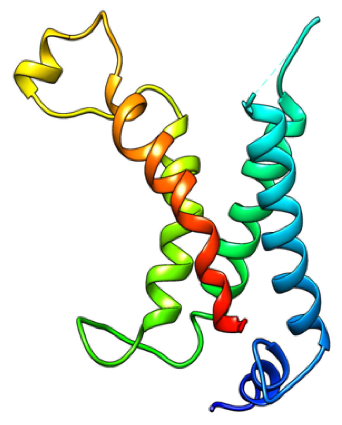
While not directly relevant to quantum calculations, there is additional evidence that directly suggests proton transport in the VSD. (1) A mutation of the first arginine in S4 (as noted in the caption to Figure 1, there are three arginines that form salt bridges in S4; there is another arginine above those, which is the one we are discussing here) into histidine produces a proton channel, and mutating neighboring residues does not do so, so the proton is moving, not merely being carried by histidine [27,28,29]. (2) The voltage gated proton channel H_v1 is very similar to the upper part of the VSD [30,31], where we find the proton cascade begins. (3) Zhao and Blunck have shown that an isolated VSD forms a cation channel, with a strong preference for protons [32].

Another interesting mutation comes from the observation that much of the evidence for the standard gating models comes from substituting cysteine for arginine, mainly in the S4 transmembrane segment. The cysteine, after it ionizes, can react with methanethiosulfonate (MTS) reagents; the MTS reagent generally appeared to react with some cysteines from the extracellular side when the channel was open, from the intracellular side when it is closed. This was interpreted as meaning that the S4 helix had moved from down (closed) to up (open). We use the usual convention that down equals intracellular, and up extracellular. However, the cysteine side chain, after ionization, is essentially a single sulfur atom, while the arginine side chain is about as large as an entire MTS reagent headgroup, the part that reacts. What this huge change in molecular volume does to the conformation of the VSD is not clear; if it does nothing, it leaves a space large enough for the MTS reagent to enter. In either case, the effect on the apparent binding of the reagent is not so easy to interpret. In order to deal with this volume effect, Bezanilla and coworkers replaced arginine with the synthetic amino acid citrulline, in which only three atoms are changed; this is a major change, however, in that it removes a charge, changing from a base (arginine) to a neutral amide without changing the side chain volume. This did have an effect on gating current, moving the curve left (i.e., the channel opens more easily). On standard models, this is a puzzle. We have performed calculations on this system, and determined the energy of the mutant, compared with the wild type. Again, the calculation was in accord with our model, which gave the qualitatively correct result [33]; while no quantitative test was possible, even a qualitative agreement seems very difficult in the standard models, while it is natural on our model.

Another mutant, in which an -OH was removed from a proton path (mutation: Y266F, using the 3Lut numbering for the K_v1.2 potassium channel), should make it more difficult to open the channel (right shift the gating current—voltage curve) on our model, but should make it easier to open on standard models (removing the -OH should make S4 slide more easily). Experimentally, Bassetto and Bezanilla (private communication) found a right shift as predicted by our model [33].

More evidence could be adduced, but it carries us away from the main point of this discussion. The additional evidence concerns the effects of mutations carried out by a number of workers, and although it is much more consistent with the proton gating current model than with the standard models, it is not directly relevant to the question of quantum effects.

4. Summary on Quantum Calculations and Effects

Taking these together, the evidence for requiring quantum calculations to accurately represent the behavior of ion channels is strong, and the evidence for tunneling is also strong, albeit not yet conclusive. It is likely that there is a threshold that is associated with proton tunneling, which would be the first step in a proton cascade. There is no evidence suggesting quantum entanglement. MD simulations, using classical force fields, no matter how modified to allow for quantum contributions for the forces, are unlikely to provide an adequate representation of the channel properties. This is not to say that MD simulations are without value; they work very well in many situations and are being continually modified to improve them. However, it appears that at present, quantum calculations are required for accurate results on ion channel gating and conduction and should benefit greatly from improvements in computer capacity.

The quantum calculations described here are optimizations that find the energy minimum of the system in several states. These are static calculations but can in principle be extended to find rates (those that do not involve tunneling) by calculating the transition states of the system between successive minima. In order to find the correct transition state, with correct activation energy, we should also calculate the free energy at the appropriate temperature, which requires at least a normal coordinate analysis. Finding a transition state translates from a microscopic to a macroscopic viewpoint, but this is too difficult for our present computational facility. Estimating rates awaits the ability to find transition states. The tunneling calculation itself describes a very rapid process, but does not allow us to say more than that it is very rapid; while it is not possible to give a time scale, it can be considered fast compared with any other process in the system, which is sufficient for our purposes. MD simulations are done as a function of time, and can now reach into the tens, or for systems that are not too large, hundreds of microseconds; as computers become more powerful, this time scale will be extended. The problems of using classical mechanics to describe charge transfer, chemical bonding, including hydrogen bonding, will remain, however, until such time as it is possible to do ab initio MD on a large enough scale. At present, for all the reasons cited earlier, only quantum calculations are reasonably likely to give correct results where hydrogen bonding, chemical bonding, and charge transfer are involved, regardless of the time scale. While we discussed this only in the context of ion channels, the same would be true of chemical reactions more generally.

The computations that have been done so far use a specific voltage gated channel, the potassium channel K_v1.2. Almost everything that is complete is done on a section of the VSD, and on the pore of this channel; the transmembrane helices that comprise the VSD are shown in Figure 1.

There is a bacterial potassium channel, designated KcsA [34] which has an almost identical selectivity filter, a somewhat smaller pore cavity, and which is gated by a drop in pH; it lacks a voltage sensing domain. We have also done calculations on KcsA, principally relevant to conduction through the pore.

5. Examples of the Type of Quantum Computations That Can Be Done

5.1. A First Example

Here, is an example of a computation that has been completed on the pore of a K⁺ channel. The pore is that of a eukaryotic voltage-gated potassium channel, K_v1.2. The selectivity filter is essentially identical to that of all potassium channels, even a viral channel [35], but the cavity at the center of the pore is somewhat larger than that of the bacterial channel, KcsA, which has a pore that is otherwise similar.

Figure 2 shows five positions of the potassium ion in a 457-atom calculation of the cavity in the channel between the gate and the selectivity filter. The entire calculated system is shown in Figure 2A, without an ion. The other five panels show five positions of the ion, showing only the water, with the protein removed, except at the upper (extracellular) end. The important point to observe is the structure of the water as the ion moves up. The middle position (Figure 2D) is an energy minimum. The energy is closely related to the water structure, which is to a large extent determined by its relation to the protein, however, as can be seen, it rearranges to hydrate the ion as it moves upward. The other key feature is the “basket” of water, which is hydrogen bonded to the threonine oxygens at the entrance to the selectivity filter. This structure is also seen in the bacterial KcsA potassium channel, which has an almost identical selectivity filter.

5.2. The Pore of the K_v1.2 Channel

The K_v1.2 channel, like all potassium channels, has a conserved TVGYG (threonine–valine–glycine–tyrosine–glycine) amino acid sequence at the entrance to the selectivity filter at the extracellular end; this is identical to the sequence in the KcsA bacterial channel. The eukaryotic K_v1.2 channel has an appreciably larger cavity in the center of the pore, containing more water, as seen in Figure 2.

Figure 3 shows a ribbon diagram of two out of four of the pore lining domains.

We also carried out calculations on ion transport in the channel pore. Figure 2 and Figure 3 show the pore. Figure 3 shows an outline of the structure of part of the selectivity filter, but not a calculation, for the eukaryotic K_v1.2 channel. Additional calculations are in progress on this pore. The basket, as shown in Figure 2 at the top of the cavity, is also found below the selectivity filter in KcsA. The calculations so far also show a mechanism for rectification, in which the ion is prevented from returning down the pore; this involves the solvation of the ion, which must be transferred from water in the cavity to threonine carbonyl groups at the entrance to the selectivity filter. Water also goes through the selectivity filter and plays a key role in rectification. As calculations progress, we will have a detailed picture of the entire process.

5.3. Calculations on the Proton Path That Leads to Voltage Gating

Calculations on the proton path that leads to voltage gating began some time ago as well. In Figure 4, we show the key first step in a proton cascade [33].

Once one has the proton shift in the VSD, one can postulate a path for the proton to the gate, which is essentially square, and has, for each domain, two prolines and two valines, the PVPV structure discussed earlier. As a sample, the X-ray structure of the open gate, and the end of one of two postulated paths to the gate, is shown in Figure 5. The important point is that two such paths can be found, in which proton transitions to residues that can act as acid/base and transmit the proton onward at certain positions. This requires the aid of the water molecules that are expected to solvate polar residues, but this has not yet been calculated. The accompanying path (not shown) has also not yet been calculated. The proposed paths are, for the present, hypothetical. However, these paths seem extremely plausible. Calculations are ongoing.

6. Summary

6.1. Quantum Calculations Are Necessary to Get Adequate Accuracy in Ion Channel Computations

Quantum calculations are necessary to obtain adequate accuracy in ion channel computations. Charge transfer cannot be properly treated classically, even with polarization. Unlike MD simulations, QM calculations do not have problems with reversibility. Ion channels can be calculated with appropriate potentials; most published MD calculations use potentials that are about an order of magnitude too high.

6.2. Errors in QM Calculations

We also discussed the types of errors found in quantum calculations, which do exist, notably the fact that the calculations are done at 0 K, due to computer limitations; the most important limitation is the size of the system that can be calculated. However, this can be overcome with more powerful computational facilities, and these are now being built. The problems in any classical calculation are inherent in the classical approximation, and in principle cannot be remedied, although excellent approximations are possible for some systems; generally, these systems are more homogenous than ion channels. As applied to a system, like ion channels, in which specific bonds, and proton transfers, are critical, these errors are critical; the classical results cannot be relied on for such systems.

6.3. Gating in Ion Channels

Gating in ion channels, based on these calculations, appears to depend on a proton cascade that begins with a proton tunneling event. The protons transfer to allow ion passage based on the removal of two or possibly three protons from the neighborhood of the gate.

We gave examples of the kind of results that it is possible to achieve with quantum computation on parts of ion channels.

References

1. Prajapati, J.D.; Mele, C.; Aksoyoglu, M.A.; Winterhalter, M.; Kleinekathöfer, U. Computational Modeling of Ion Transport in Bulk and through a Nanopore Using the Drude Polarizable Force Field. J. Chem. Inf. Model. 2020, 60, 3188–3203. [Google Scholar] [CrossRef] [PubMed]
2. Ocello, R.; Furini, S.; Lugli, F.; Recanatini, M.; Domene, C.; Masetti, M. Conduction and Gating Properties of the TRAAK Channel from Molecular Dynamics Simulations with Different Force Fields. J. Chem. Inf. Model. 2020, 60, 6532–6543. [Google Scholar] [CrossRef] [PubMed]
3. Furini, S.; Domene, C. Critical Assessment of Common Force Fields for Molecular Dynamics Simulations of Potassium Channels. J. Chem. Theory Comput. 2020, 16, 7148–7159. [Google Scholar] [CrossRef] [PubMed]
4. Sansom, M.S.P.; Bond, P.J.; Deol, S.S.; Grottesi, A.; Haider, S.; Sands, Z.A. Molecular simulations and lipid-protein interactions: Potassium channels and other membrane proteins. Biochem. Soc. Trans. 2005, 33, 916–920. [Google Scholar] [CrossRef]
5. Allison, J.R. Computational methods for exploring protein conformations. Biochem. Soc. Trans. 2020, 48, 1707–1724. [Google Scholar] [CrossRef] [PubMed]
6. Bumbacila, B.; Putz, M.V. Monte Carlo Molecular Simulations; Apple Academic Press Inc.: Palm Bay, FL, USA, 2020. [Google Scholar]
7. Horsewill, A.J. Quantum Molecular Tunneling Studied by Field-cycling NMR. New Dev. NMR 2019, 18, 405–426. [Google Scholar]
8. Sharma, V.K.; Srinivasan, H.; Sakai, V.G.; Mitra, S. Dioctadecyldimethylammonium bromide, a surfactant model for the cell membrane: Importance of microscopic dynamics. Struct. Dyn. 2020, 7, 051301. [Google Scholar] [CrossRef]
9. Bucher, D.; Guidoni, L.; Carloni, P.; Rothlisberger, U. Coordination Numbers of K+ and Na+ Ions Inside the Selectivity Filter of the KcsA Potassium Channel: Insights from First Principles Molecular Dynamics. Biophys. J. 2010, 98, L47–L49. [Google Scholar] [CrossRef] [Green Version]
10. Cholasseri, R.; De, S. Dual-Site Binding of Quaternary Ammonium Ions as Internal K+-Ion Channel Blockers: Nonclassical (C–H··· O) H Bonding vs Dispersive (C–H··· H–C) Interaction. J. Phys. Chem. B 2021, 125, 86–100. [Google Scholar] [CrossRef] [PubMed]
11. Carnevale, V.; Fiorin, G.; Levine B., G.; Degrado W., F.; Klein, M. Multiple Proton Confinement in the M2 Channel from the Influenza A Virus. J. Phys. Chem.C Nanomater. Interfaces 2010, 114, 20856–20863. [Google Scholar] [CrossRef] [Green Version]
12. Masetti, M.; Berti, C.; Ocello, R.; Di Martino, G.P.; Recanatini, M.; Fiegna, C.; Cavalli, A. Multiscale Simulations of a Two-Pore Potassium Channel. J. Chem. Theory Comput. 2016, 12, 5681–5687. [Google Scholar] [CrossRef] [PubMed]
13. Qi, Y.; Cheng, X.; Han, W.; Jo, S.; Schulten, K.; Im, W. CHARMM-GUI PACE CG Builder for Solution, Micelle, and Bilayer Coarse-Grained Simulations. J. Chem. Inf. Model. 2014, 54, 1003–1009. [Google Scholar] [CrossRef] [PubMed]
14. Vianello, R.; Domene, C.; Mavri, J. The Use of Multiscale Molecular Simulations in Understanding a Relationship between the Structure and Function of Biological Systems of the Brain: The Application to Monoamine Oxidase Enzymes. Front. Neurosci. 2016, 10, 327. [Google Scholar] [CrossRef] [Green Version]
15. Von Wegner, F.; Wieder, N.; Fink, R.H.A. Simulation strategies for calcium microdomains and calcium-regulated calcium channels. Adv. Exp. Med. Biol. 2012, 740, 553–567. [Google Scholar]
16. Frisch, M.J.; Trucks, G.W.; Schlegel, H.B.; Scuseria, G.E.; Robb, M.A.; Cheeseman, J.R.; Scalmani, G.; Barone, V.; Mennucci, B.; Petersson, G.A.; et al. Gaussian 09, Revision D.01. 2009; Gaussian, Inc.: Wallingford, CT, USA, 2013. [Google Scholar]
17. Weinhold, F. Natural bond orbital analysis: A critical overview of relationships to alternative bonding perspectives. J. Comput. Chem. 2012, 33, 2363–2379. [Google Scholar] [CrossRef]
18. Olshanii, M. Back of the Envelope Quantum Mechanics; World Scientific: Singapore, 2014. [Google Scholar]
19. Asamoah, O.K.; Wuskell, J.P.; Loew, L.M.; Bezanilla, F. A Fluorometric Approach to Local Electric Field Measurements in a Voltage-Gated Ion Channel. Neuron 2003, 37, 85–98. [Google Scholar] [CrossRef] [Green Version]
20. Georgiev, D.D.; Kolev, S.K.; Cohen, E.; Glazebrook, J.F. Computational capacity of pyramidal neurons in the cerebral cortex. Brain Res. 2020, 1748, 147069. [Google Scholar] [CrossRef]
21. Sigg, D.; Bezanilla, F.; Stefani, E. Fast gating in the Shaker K+ channel and the energy landscape of activation. Proc. Natl. Acad. Sci. USA 2003, 100, 7611–7615. [Google Scholar] [CrossRef] [Green Version]
22. Sigg, D.; Bezanilla, F.; Stefani, E. Temperature dependence of the early component of gating currents from Shaker K chaznnels. Biophys. J. 2001, 80, 219a. [Google Scholar]
23. Fatade, A.; Snowhite, J.; Green, M.E. A Resonance Model gives the Response to Membrane Potential for an Ion Channel: II. Simplification of the Calculation, and Prediction of Stochastic Resonance. J. Theor. Biol. 2000, 206, 387–393. [Google Scholar] [CrossRef] [PubMed]
24. Fohlmeister, J.; Adelman, W. Gating current harmonics. I. Sodium channel activation gating in dynamic steady states. Biophys. J. 1985, 48, 375–390. [Google Scholar] [CrossRef] [Green Version]
25. Fohlmeister, J.; Adelman, W. Gating current harmonics. II. Model simulations of axonal gating currents. Biophys. J. 1985, 48, 391–400. [Google Scholar] [CrossRef] [Green Version]
26. Bezrukov, S.M.; Vodyanoy, I. Stochastic resonance in non-dynamical systems without response thresholds. Nat. Cell Biol. 1997, 385, 319–321. [Google Scholar]
27. Starace, D.; Stefani, E.; Bezanilla, F. Histidine scanning mutagenesis indicates full translocation of two charges of the Shaker K channel voltage sensor. Biophys. J. 1998, 74, A215. [Google Scholar]
28. Starace, D.M.; Bezanilla, F. A proton pore in a potassium channel voltage sensor reveals a focused electric field. Nat. Cell Biol. 2004, 427, 548–553. [Google Scholar] [CrossRef] [PubMed]
29. Starace, D.M.; Stefani, E.; Bezanilla, F. Voltage-Dependent Proton Transport by the Voltage Sensor of the Shaker K+ Channel. Neuron 1997, 19, 1319–1327. [Google Scholar] [CrossRef] [Green Version]
30. Ramsey, I.S.; Mokrab, Y.; Carvacho, I.; Sands, Z.A.; Sansom, M.S.P.; Clapham, D.E. An aqueous H+ permeation pathway in the voltage-gated proton channel Hv1. Nat. Struct. Mol. Biol. 2010, 17, 869–875. [Google Scholar] [CrossRef] [PubMed] [Green Version]
31. Okamura, Y.; Fujiwara, Y.; Sakata, S. Gating Mechanisms of Voltage-Gated Proton Channels. Annu. Rev. Biochem. 2015, 84, 685–709. [Google Scholar] [CrossRef]
32. Zhao, J.; Blunck, R. The isolated voltage sensing domain of the Shaker potassium channel forms a voltage-gated cation channel. eLife 2016, 5, e18130. [Google Scholar] [CrossRef]
33. Kariev, A.M.; Green, M.E. Quantum Calculation of Proton and Other Charge Transfer Steps in Voltage Sensing in the Kv1.2 Channel. J. Phys. Chem. B 2019, 123, 7984–7998. [Google Scholar] [CrossRef]
34. Kariev, A.M.; Znamenskiy, V.S.; Green, M.E. Quantum mechanical calculations of charge effects on gating the KcsA channel. Biochim. Biophys. Acta BBA Biomembr. 2007, 1768, 1218–1229. [Google Scholar] [CrossRef] [PubMed] [Green Version]
35. Hertel, B.; Tayefeh, S.; Kloss, T.; Hewing, J.; Gebhardt, M.; Baumeister, D.; Moroni, A.; Thiel, G.; Kast, S.M. Salt bridges in the miniature viral channel Kcv are important for function. Eur. Biophys. J. 2009, 39, 1057–1068. [Google Scholar] [CrossRef]
36. Kariev, A.M.; Green, M.E. K+ in a Kv1.2 Channel Pore: Hydration, Selectivity, and the Role of a Conserved Threonine. bioRxiv 2018. [Google Scholar] [CrossRef]
Figure 1. The four helices that comprise the transmembrane part of the voltage sensing domain in Kv1.2. In standard gating models, the S4 helix, shown here in red, moves down perhaps 10 Å (the exact distance depends on the version of the standard model), and may twist, or turn into a 310 helix, or otherwise rearrange. There are salt bridges between positive charges, three arginines, on S4 and negative charges on the other helices, which would have to break for this motion to occur, and then reform correctly thousands of times. In the model we propose, the conformation remains fixed but protons move to provide the measured gating current.
Symmetry 13 00655 g001
Figure 2. Water molecules in the cavity with the ion in five positions: (A) includes the protein and is shown in a smaller scale than for (B) through (F), for which all but the bottom of the SF (top, threonine carbons green), and (bottom) one proline (purple) of the PVPV sequence at the gate (P = proline, V = valine; each domain has a PVPV sequence at the gate), are removed for clarity. The ion is shown as a purple sphere; positions are at approximately 2 Å above the PVPV region in (B), and at 2 Å intervals above that ((C) through (F)): K+ ion approximate positions above the PVPV gate are (C): 4 Å; (D) 6 Å; (E) 8 Å; (F) 10 Å)). Dotted lines show hydrogen bonds, small red circles water oxygens (cavity), light blue, (F) only, basket water interacting with the K+; large red circles, special threonine oxygens, as labeled. This is reproduced from Kariev and Green [36].
Symmetry 13 00655 g002
Figure 3. The pore section of the Kv1.2 channel, showing 2 of the 4 domains. The selectivity filter is at the top center (note the purple spheres—upper center-- that denote the position of energy minima for the ion, or for water molecules, within the filter. In the center is the cavity, which holds several dozen water molecules, and may hold a potassium ion in addition. At the bottom is the gate, which must open to allow a K+ ion to enter, and close to prevent K+ from entering the channel and thus leaving the cell. The orientation, as always, is extracellular up, intracellular down.
Symmetry 13 00655 g003
Figure 4. The effect of a single proton shift as optimized starting from the X-ray structure; a proton path through the protein and water, and on to the gate, is not hard to find.
Symmetry 13 00655 g004
Figure 5. The X-ray structure of the gate in the open state: The two asparagines (N412, N414) are a part of the end of the proton path. All colored residues are part of the path. A K+ ion (magenta sphere, center) is shown at the center of the gate, which in the X-ray structure (open state) has a diagonal distance of 15.65 Å. The view is from the intracellular end, looking into the pore, which continues into the plane of the paper.
Symmetry 13 00655 g005
Publisher’s Note: MDPI stays neutral with regard to jurisdictional claims in published maps and institutional affiliations.