
A Bimodal Extension of the Exponential Distribution with Applications in Risk Theory


Abstract
:1. Introduction
2. Bimodal Extension of the Exponential Distribution
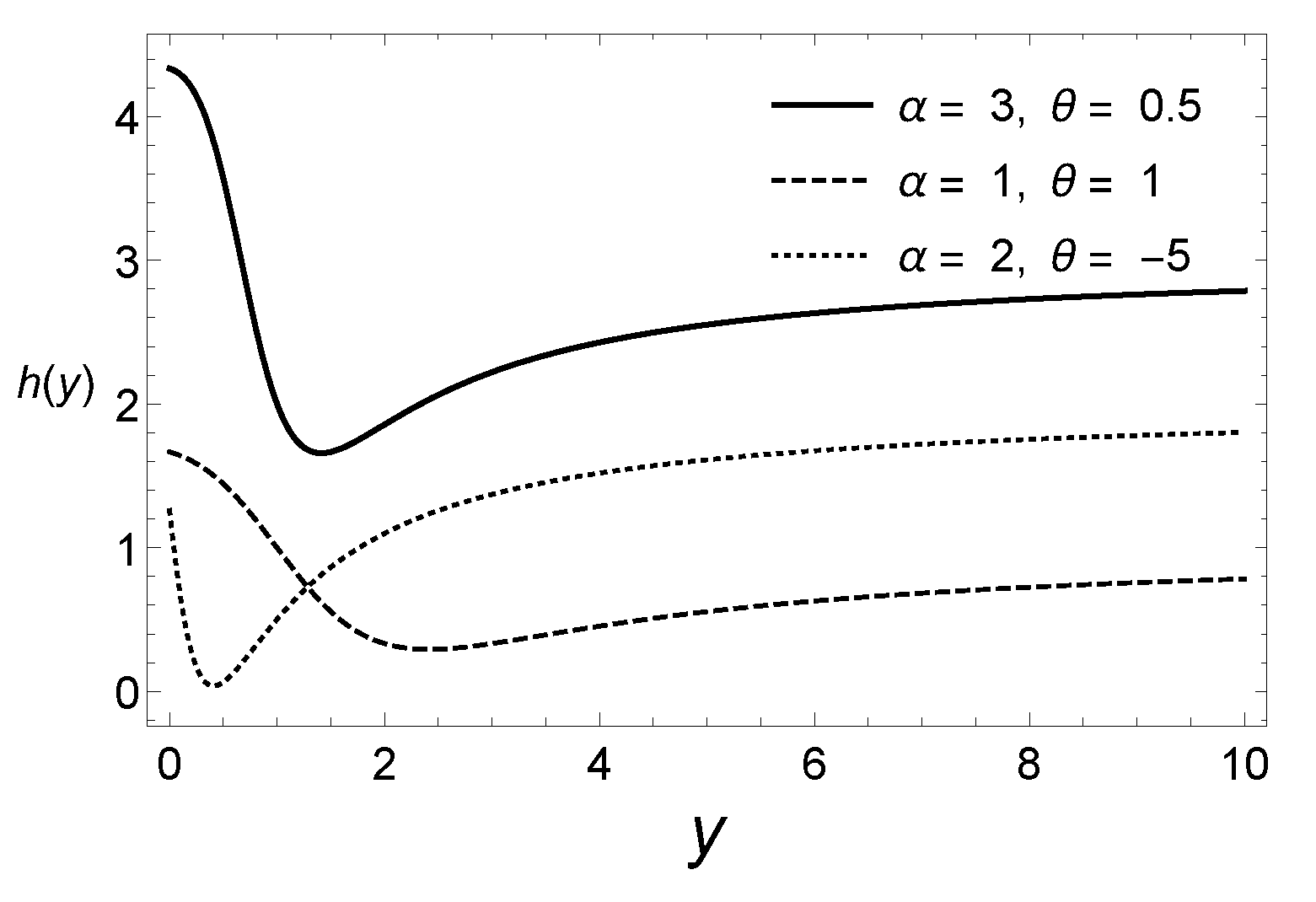
Reliability, Hazard Rate Function and Moments
3. Results in Risk Theory
4. Methods of Estimation and Simulation
Simulation Experiment
5. A suitable Regression Model
6. Empirical Results
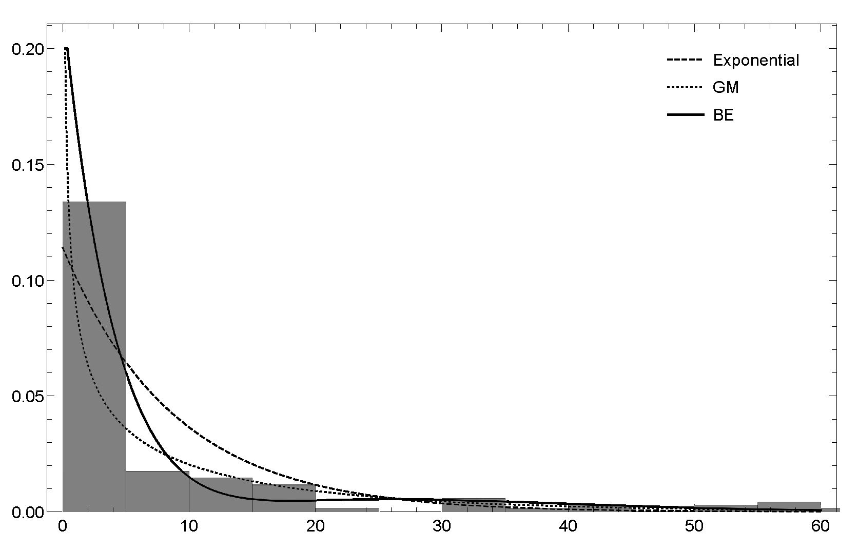
6.1. Dataset 1
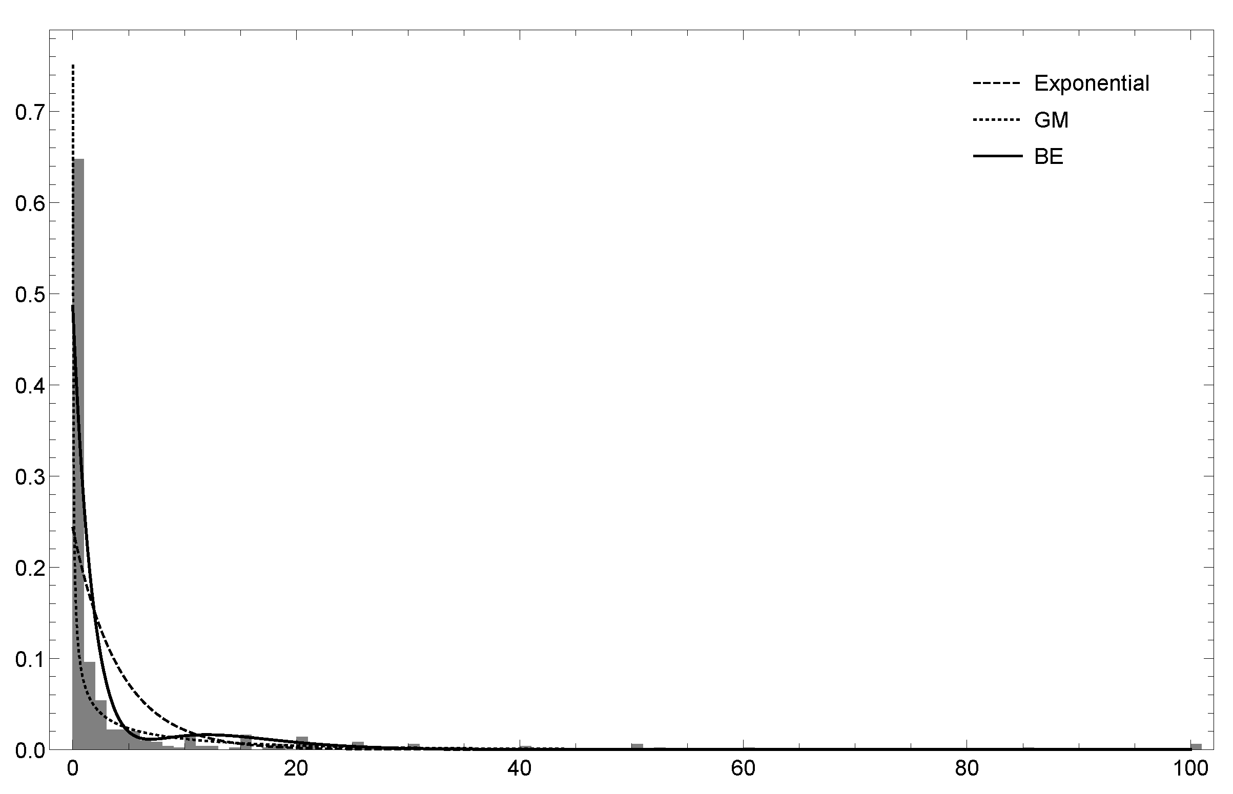
6.2. Dataset 2
7. Conclusions and Extensions
Author Contributions
Funding
Institutional Review Board Statement
Informed Consent Statement
Data Availability Statement
Acknowledgments
Conflicts of Interest
References
- Kumbhakar, S.; Parmeter, C.; Tsionas, E.G. A zero inefficiency stochastic frontier model. J. Econ. 2013, 172, 66–76. [Google Scholar] [CrossRef]
- Tong, N.; Christophe, M.; Thomas, L. A zero-adjusted gamma model for mortgage loan loss given default. Int. J. Forecast. 2013, 29, 548–562. [Google Scholar] [CrossRef] [Green Version]
- Elal-Olivero, D. Alpha-skew-normal distribution. Proyecciones 2010, 29, 224–240. [Google Scholar] [CrossRef] [Green Version]
- Marshall, A.; Olkin, I. A new method for adding a parameter to a family of distributions with application to the exponential and Weibull families. Biometrika 1997, 84, 641–652. [Google Scholar] [CrossRef]
- Gupta, P.K.; Kundu, D. Generalized exponential distributions. Aust. N. Z. J. Stat. 1999, 41, 173–188. [Google Scholar] [CrossRef]
- Gómez-Déniz, E. Adding a parameter to the exponential and Weibull distributions with applications. Math. Comput. Simul. 2017, 144, 108–119. [Google Scholar] [CrossRef]
- Kuhn, D.; Mohajerin, P.; Nguyen, V.; Abadeh, S. Wasserstein Distributionally Robust Optimization: Theory and Applications in Machine Learning. In Operations Research & Management Science in the Age of Analytics; Informs: Catonsville, MD, USA, 2019; pp. 130–166. [Google Scholar]
- Imani, M.; Ghoreishi, S. Scalable Inverse Reinforcement Learning Through Multifidelity Bayesian Optimization. IEEE Trans. Neural Netw. Learn. Syst. 2021, 1–8. [Google Scholar] [CrossRef]
- Bellemare, M.G.; Dabney, W.; Munos, R. A Distributional Perspective on Reinforcement Learning. In Proceedings of the 34th International Conference on Machine Learning, Sydney, NSW, Australia, 6–11 August 2017; Precup, D., Teh, Y.W., Eds.; International Convention Centre: Sydney, NSW, Australia, 2017; Volume 70, pp. 449–458. [Google Scholar]
- Fisher, R. The effects of methods of ascertainmenut pon the estimation of frequencies. Ann. Eugen. 1934, 6, 13–25. [Google Scholar] [CrossRef]
- Harandi, S.S.; Alamtsaz, M. Discrete alpha-skew-Laplace distribution. SORT 2013, 39, 71–84. [Google Scholar]
- Patil, G.; Rao, C. Weighted distributions and size biased sampling with applications to wildlife populations and human families. Biometrics 1978, 34, 179–184. [Google Scholar] [CrossRef] [Green Version]
- Hogg, R.; Klugman, S. Loss Distributions; John Wiley and Sons: New York, NY, USA, 1984. [Google Scholar]
- Boland, P. Statistical and Probabilistic Methods in Actuarial Science; Chapman & Hall: London, UK, 2007. [Google Scholar]
- Klugman, S.; Panjer, H.; Willmot, G. Loss Models: From Data to Decisions, 3rd ed.; Wiley: Hoboken, NJ, USA, 2008. [Google Scholar]
- Von Newmann, J. Various Techniques used in Connection With Random Digits. Stand. Appl. Math. Ser. 1951, 12, 36–38. [Google Scholar]
- Ruskeepaa, H. Mathematica Navigator. Mathematics, Statistics, and Graphics, 3rd ed.; Academic Press: Cambridge, MA, USA, 2009. [Google Scholar]
- Brooks, C. RATS Handbook to Accompany Introductory Econometrics for Finance; Cambridge University Press: Cambridge, UK, 2009. [Google Scholar]
- Dean, C.; Lawless, J.; Willmot, G. A mixed Poisson-inverse-Gaussian regression model. Can. J. Stat. 1989, 17, 171–181. [Google Scholar] [CrossRef]
- Vuong, Q. Likelihood ratio tests for model selection and non-nested hypothesesl. Econometrica 1989, 57, 307–333. [Google Scholar] [CrossRef] [Green Version]
- Scollnik, D. On composite Lognormal-Pareto models. Scand. Actuar. J. 2007, 1, 20–33. [Google Scholar] [CrossRef]
- Scollnik, D.; Sun, C. Modeling with Weibull-Pareto models. N. Am. Actuar. J. 2012, 16, 260–272. [Google Scholar] [CrossRef]


| (SD)(C) | (SD)(C) | (SD)(C) | (SD)(C) | ||
| 1.0 | 1.0 | 1.0415(0.1793)(92.9) | 0.9997(0.2508)(95.3) | 1.0128(0.1042)(94.1) | 0.990155(0.1579)(94.6) |
| 2.0 | 1.0133(0.1021)(93.5 | 2.0564(0.4298)(94.7) | 1.0040(0.0701)(95.0) | 2.0488(0.2953)(96.0) | |
| 3.0 | 1.0063(0.0856)(94.3) | 3.1707(0.8710)(94.0) | 1.0051(0.0600)(95.2) | 3.0881(0.5573)(94.9) | |
| 2.0 | 1.0 | 2.0615(0.3737)(93.8) | 0.9813(0.2605)(94.7) | 2.0262(0.2094)(93.4) | 0.9971(0.1579)(93.9) |
| 2.0 | 2.0133(0.2013)(93.9) | 2.0671(0.4328)(94.6) | 2.0083(0.1414)(95.4) | 2.0266(0.2916)(95.3) | |
| 3.0 | 2.0147(0.1718)(95.5) | 3.2368(0.9209)(92.9) | 2.0101(0.1200)(94.0) | 3.0804(0.5570)(94.5) | |
| 3.0 | 1.0 | 3.1000(0.5494)(93.1) | 1.0011(0.2582)(96.3) | 3.0544(0.3125)(94.2) | 1.0085(0.1573)(95.4) |
| 2.0 | 3.0277(0.3052)(93.9) | 2.0567(0.4303)(92.8) | 3.0265(0.2130)(95.1) | 2.0296(0.2919)(95.9) | |
| 3.0 | 3.0013(0.2545)(95.8) | 3.2297(0.8992)(94.6) | 3.0076(0.1795)(95.2) | 3.1114(0.5715)(94.4) | |
| (SD)(C) | (SD)(C) | (SD)(C) | (SD)(C) | ||
| 1.0 | 1.0 | 1.0139(0.0843)(93.3) | 1.0097(0.1275)(95.3) | 1.0092(0.0731)(95.8) | 1.0014(0.1098)(92.8) |
| 2.0 | 1.0023(0.0574)(94.4) | 2.0158(0.2348)(95.4) | 1.0029(0.0495)(95.2) | 2.0255(0.2039)(95.2) | |
| 3.0 | 1.0010(0.0485)(95.4) | 3.0794(0.4495)(95.3) | 1.0030(0.0422)(93.5) | 3.0395(0.3785)(95.3) | |
| 2.0 | 1.0 | 2.0184(0.1696)(95.1) | 0.9979(0.1271)(94.2) | 2.0096(0.1457)(95.3) | 1.0011(0.1098)(95.7) |
| 2.0 | 2.0068(0.1147)(95.6) | 2.0116(0.2336)(95.9) | 2.0063(0.0992)(93.2) | 2.0133(0.2020)(95.3) | |
| 3.0 | 2.0016(0.0972)(95.2) | 3.0647(0.4466)(94.7) | 2.0059(0.0844)(95.3) | 3.0312(0.3763)(94.8) | |
| 3.0 | 1.0 | 3.0231(0.2533)(94.5) | 0.9943(0.1265)(95.2) | 3.0227(0.2193)(95.9) | 1.0037(0.1100)(95.5) |
| 2.0 | 3.0051(0.1719)(93.9) | 2.0268(0.2365)(96.0) | 3.0016(0.1486)(95.2) | 2.0109(0.2017)(95.1) | |
| 3.0 | 3.0030(0.1458)(94.5) | 3.0851(0.4518)(95.8) | 2.9982(0.1261)(95.9) | 3.0397(0.3784)(93.6) |
| Variable | Description |
|---|---|
| Gender | Gender of the survey respondent |
| Age | Age of the survey respondent |
| Marstat | Marital status of the survey respondent |
| (=1 if married, =2 if living with partner, and =0 otherwise) | |
| Education | Number of years of education of the survey respondent |
| Ethnicity | Ethnicity |
| Smarstat | Marital status of the respondent’s spouse |
| Sgender | Gender of the respondent’s spouse |
| Sage | Age of the respondent’s spouse |
| Seducation | Education of the respondent’s spouse |
| Numhh | Number of household members |
| Income | Annual income of the family |
| Totincome | Total income |
| Charity | Charitable contributions |
| Dataset 1 | Dataset 2 | |||||
|---|---|---|---|---|---|---|
| Exponential | Exponential | |||||
| 0.243 | 1.534 | 0.285 | 0.114 | 1.353 | 0.129 | |
| (0.011) | (0.053) | (0.012) | (0.009) | (0.076) | (0.014) | |
| - | 7.475 | 1.429 | - | 10.893 | 1.172 | |
| - | (0.691) | (0.091) | - | (1.412) | (0.169) | |
| - | 0.45 | - | 0.198 | |||
| - | (0.022) | - | (0.034) | |||
| −1206.92 | −1073.63 | −959.524 | −430.685 | −419.870 | −393.317 | |
| AIC | 2415.84 | 2153.26 | 1923.05 | 863.369 | 845.741 | 790.635 |
| CAIC | 2421.05 | 2168.90 | 1933.48 | 867.282 | 857.479 | 798.460 |
| Variable | Estimate | S.E. | -Statistic | |
|---|---|---|---|---|
| gender | 1.688 (1.023) | 0.190 (0.192) | 8.879 (5.308) | 0.00 (0.00) |
| age | −0.023 (0.018) | 0.007 (0.007) | 3.371 (2.618) | 0.00 (0.00) |
| marstat | −1.639 (−1.310) | 0.158 (0.189) | 10.344 (6.906) | 0.00 (0.01) |
| education | 0.206 (0.221) | 0.019 (0.019) | 10.622 (11.462) | 0.00 (0.00) |
| ethnicity | 0.002 (−0.128) | 0.032 (0.035) | 0.078 (3.622) | 0.93 (0.00) |
| smarstat | 0.201 (0.613) | 0.112 (0.111) | 1.789 (5.487) | 0.07 (0.00) |
| sgender | −1.132 (0.031) | 0.268 (0.296) | 4.223 (0.104) | 0.00 (0.91) |
| sage | 0.048 (0.010) | 0.007 (0.008) | 6.093 (1.287) | 0.00 (0.19) |
| seducation | 0.134 (0.044) | 0.020 (0.024) | 6.492 (1.821) | 0.00 (0.07) |
| numhh | −0.126 (0.145) | 0.034 (0.044) | 3.679 (3.282) | 0.00 (0.00) |
| income | 0.261 (0.369) | 0.030 (0.030) | 8.730 (12.053) | 0.00 (0.00) |
| totincome | 0.125 (0.097) | 0.037 (0.037) | 3.348 (2.616) | 0.00 (0.01) |
| charity | −0.612 (−0.630) | 0.106 (0.122) | 5.762 (5.170) | 0.00 (0.00) |
| 1.495 | 0.102 | 14.646 | 0.00 | |
| constant | −5.018 (−8.959) | 0.585 (0.519) | 8.570 (17.246) | 0.00 (0.00) |
| Variable | Description |
|---|---|
| km | Distance driven by a vehicle, grouped into five categories |
| zone | Graphic zone of a vehicle, grouped into seven categories |
| bonus | Driver claim experience, grouped into seven categories |
| make | Type of a vehicle |
| claims | Number of claims |
| Variable | Estimate | S.E. | -Statistic | |
|---|---|---|---|---|
| km | −0.303 (−0.290) | 0.070 (0.076) | 4.303 (3.824) | 0.00 (0.00) |
| zone | −0.335 (−0.255) | 0.049 (0.052) | 6.707 (4.887) | 0.00 (0.00) |
| make | −0.030 (−0.206) | 0.056 (0.079) | 0.535 (2.588) | 0.59 (0.01) |
| claims | 0.034 (0.027) | 0.004 (0.004) | 8.400 (6.759) | 0.00 (0.00) |
| 1.799 | 0.226 | 7.932 | 0.00 | |
| constant | 2.752 (3.044) | 0.479 (0.481) | 5.735 (6.317) | 0.00 (0.00) |
Publisher’s Note: MDPI stays neutral with regard to jurisdictional claims in published maps and institutional affiliations. |
© 2021 by the authors. Licensee MDPI, Basel, Switzerland. This article is an open access article distributed under the terms and conditions of the Creative Commons Attribution (CC BY) license (https://creativecommons.org/licenses/by/4.0/).
Share and Cite
Reyes, J.; Gómez-Déniz, E.; Gómez, H.W.; Calderín-Ojeda, E. A Bimodal Extension of the Exponential Distribution with Applications in Risk Theory. Symmetry 2021, 13, 679. https://doi.org/10.3390/sym13040679
Reyes J, Gómez-Déniz E, Gómez HW, Calderín-Ojeda E. A Bimodal Extension of the Exponential Distribution with Applications in Risk Theory. Symmetry. 2021; 13(4):679. https://doi.org/10.3390/sym13040679
Chicago/Turabian StyleReyes, Jimmy, Emilio Gómez-Déniz, Héctor W. Gómez, and Enrique Calderín-Ojeda. 2021. "A Bimodal Extension of the Exponential Distribution with Applications in Risk Theory" Symmetry 13, no. 4: 679. https://doi.org/10.3390/sym13040679
APA StyleReyes, J., Gómez-Déniz, E., Gómez, H. W., & Calderín-Ojeda, E. (2021). A Bimodal Extension of the Exponential Distribution with Applications in Risk Theory. Symmetry, 13(4), 679. https://doi.org/10.3390/sym13040679