Constraints on Newtonian Interplanetary Point-Mass Interactions in Multicomponent Systems from the Symmetry of Their Cycles

Abstract

Interplanetary interactions are the largest forces in our Solar System that disturb the planets from their elliptical orbits around the Sun, yet are weak (<10⁻³ Solar). Currently, these perturbations are computed in pairs using Hill’s model for steady-state, central forces between one circular and one elliptical ring of mass. However, forces between rings are not central. To represent interplanetary interactions, which are transient, time-dependent, and cyclical, we build upon Newton’s model of interacting point-mass pairs, focusing on circular orbits of the eight largest bodies. To probe general and evolutionary behavior, we present analytical and numerical models of the interplanetary forces and torques generated during the planetary interaction cycles. From symmetry, over a planetary interaction cycle, radial forces dominate while tangential forces average to zero. Our calculations show that orbital perturbations require millennia to quantify, but observations are only over ~165 years. Furthermore, these observations are compromised because they are predominantly made from Earth, whose geocenter occupies a complex, non-Keplerian orbit. Eccentricity and inclination data are reliable and suggest that interplanetary interactions have drawn orbital planes together while elongating the orbits of the two smallest planets. This finding is consistent with conservation principles governing the eight planets, which formed as a system and evolve as a system.

1. Introduction and Background

Many orbits in the Solar System are well-represented by the reduced two-body approximation due to the Sun’s immense mass and large distances between objects. Evolutionary behavior is driven by the existence of secondary forces that disturb the perfect balance inherent to highly symmetrical Keplerian orbits. When secondary forces are small, these can be treated as perturbations, for which simple models provide sufficient accuracy. Previous modeling efforts and the present study consider a simplified, eight-planet system. Perturbations therein are small due to large distances between planets and their small masses compared to Solar. Confirming orbital perturbation calculations thus requires that measurements must be either highly accurate and/or be made over a long time period.

Unfortunately, observations are limited in both accuracy and duration, as exemplified by Neptune (Figure 1). Planetary and Solar motions are recorded against the stars whereby only motions perpendicular to the line-of-sight are well-resolved. Consequently, mathematical modeling and multicomponent fitting are used to extract orbital parameters from astronomical data. Processed observational data suggest that the positions of planetary perihelia are moving with time (e.g., [1]). This behavior is referred to as perihelion precession. However, only ~165 years of reliable observations exist, and most of these are made from the Earth. Although the barycenter moves in an elliptical orbit, the geocenter position is controlled by the Moon’s orbit, so Earth’s motions are not in a plane and the associated cycles are near 20 years, not annually. Hence, precession of the planets is not well recorded.

Determining changes in orbital radius are more uncertain. Only for Earth’s encircling Moon have changes in radii been directly measured, via reflections of laser light [2]. These changes are ~13 orders-of-magnitude smaller than orbital velocities, and thus are not resolvable with observational techniques. Roughly the same situation should exist in orbital radius changes from interplanetary perturbations. Theoretical models for interplanetary interactions are thus needed to understand the magnitude of the various perturbations and their evolutionary implications.

1.1. Previous Theoretical Models of Planetary Interactions

Only a few theoretical models exist that depict the perturbing forces within our eight-planet system. All models consider forces between the various pairs. All interplanetary force models neglect effects of our large and close Moon, which is a different problem [4], and view the Earth as occupying the barycenter’s orbit. Because gravitational forces between planets are tiny compared to Solar forces, interactions of pairs are independent and sum, e.g., [5]. The oblate shape of the Sun, and of the gas giants, has no effect at distances greatly exceeding body radii [6]. Thus, all models investigate the effect of a single perturbing planet (PP) on a planet of interest (POI).

Newton based his calculations on point masses, but only considered configurations where both planets are on the same side of the Sun. Gauss [7] attempted to model perihelia precession as a series of steady-state, three-body problems, each involving one elliptical ring and one circular ring of mass around a point-mass Sun. Gauss’s incomplete mathematical model was developed further by Hill [8,9] under the additional assumption of central forces (discussed below). Dolittle’s [10] application of Hill’s formulation to the rocky planets is used today with trivial modifications, such as incorporating revised planetary masses, e.g., [11,12].

Hill [8,9] assumed that planets can be modeled as if their mass were distributed in rings, and that the forces between these rings are central. Neither assumption is supportable. First, central forces only occur around points and spheres (e.g., Kellogg [13]), and do not occur around rings [14]. Elliptical rings also lack a central force field, in view of forces to the oblate not being central [6]. Second, only steady-state behavior is portrayed. Ring models were never applied to the outer Solar System because the interactions were recognized as being periodic and transient. However, the inner Solar System behaves likewise, as is evident from comparing interaction cycles to orbital periods in these two sub-systems (

Table 1. Approximate time in Julian years (i.e., Earth’s orbital period) between successive close passes, omitting duplicate entries, with comparisons to orbital periods (in italics).

Pair	Interval	Pair	Interval	Pair	Interval
Mercury–Jupiter	0.242	Mercury–Saturn	0.24	Mercury–Mars	0.307
Venus–Jupiter	0.655	Venus–Saturn	0.65	Venus–Mars	1.0
Earth–Jupiter	1.1	Earth–Saturn	1.03	Earth–Mars	2.2
Mars–Jupiter	2.25	Mars–Saturn	2.0	Uranus–Mars	1.9
Saturn–Jupiter	20.3	Uranus’ orbit	83.8	Neptune–Mars	1.88
Uranus–Jupiter	13.5	Uranus–Saturn	~45	Mars’ orbit	1.88
Neptune–Jupiter	12.6	Neptune–Saturn	~36	Neptune–Uranus	~164
Jupiter’s orbit	11.86	Saturn’s orbit	29.46	Neptune’s orbit	163.7
Mercury–Venus	0.364	Mercury–Earth	0.288	Venus–Earth	1.6

Notes: Intervals were obtained from the animated graphics of Ford [3], which spans 30 years, and so the entries for the most distant pairs are rough, as indicated. Figure 1 shows planetary positions from [3]. Other entries are reasonably accurate, but are not exact because the determinations are graphical. These cycles differ from close approaches, which are less frequent due to the influences of inclination and eccentricity. Cycles of the rocky planets with Uranus and Neptune are negligibly larger than the orbital periods of the former, so not all are listed. For Mars and beyond, orbital periods (from [15]) are given (in italics) for comparison. Uranus and Neptune are roughly in a 2:1 cycle, see Figure 1.

; Figure 2). Thus, Hill’s approximations cannot capture key behaviors.

1.2. Purpose and Organization

Constructing a time-dependent analytical formulation for interplanetary interactions and verifying it via modern numerical methods should improve our understanding of departures from Keplerian orbits and Solar System evolution. In addition, similar interactions occur in other star and planetary systems. Lastly, relativistic effects between planets are negligible (e.g., [16]), but evaluating models for the Sun’s relativistic effect on Mercury depends on accurate knowledge of interplanetary Newtonian terms. In detail, many different relativistic models exist for the Sun’s effect on Mercury (e.g., [5,11,12,17,18,19,20]), where the relativistic term for Mercury is only ~3× the uncertainty of the eight terms calculated using Hill’s problematic model.

We calculate perturbations of the eight planets’ orbits that result from Newtonian Interplanetary Point-mass Interactions (NIPIs), after Newton’s pioneering efforts. Section 2 describes the forces and implications of conservation laws, which provide a particular solution. Section 3 utilizes symmetry to probe the periodic changes in the orbits of interacting pairs. Section 4 provides numerical models of key pairs. These results confirm the findings in Section 2 and Section 3, while providing further insights. Section 5 compares our results to observational data. Section 6 covers implications.

2. Physical Principles Governing Newtonian Interplanetary Point-Mass Interactions

Our Newtonian model is based on forces and torques encountered by a pair of planets as they move from one linear alignment to the next, defined here as an interaction cycle. As adopted in previous models, perturbing forces caused by interacting pairs of point-masses are independent and sum, while the presence of Earth’s Moon is neglected.

Orbital parameters can be expressed as a diminishing series. Since interplanetary forces are tiny relative to Solar forces in the inner Solar System, only the first-order terms should be important. Most orbits are nearly circular (Figure 3a), so this case suffices in a perturbation model. Specifically, the largest eccentricity (e), of Mercury, is ~2× that of the next most eccentric orbit of Mars, where:

e = (1 − c²/a²)^½;  c = a(1 − e²)^½;  a²e² = a² − c².

(1)

The semi-major axis (a) equals the average radius. The semi-minor axis (c) of Mercury differs from a by only 2% (Figure 3b). Orbital inclinations are likewise small, reaching only ~6° for Mercury relative to Jupiter (Figure 3a). Hence, inclination is treated independently of eccentricity, which is evaluated below by approximating the orbits of a pair as co-planar.

2.1. Forces, Small and Large

Newtonian attractive forces (F) between the Sun and each planet are approximated by:

$${\overrightarrow{F}}_{S,i}=-\frac{G{M}_S{m}_i}{r_i^2} \hat{\mathrm{r}},$$

(2)

where G is the gravitational constant, M_S is solar mass, m_i is the mass of the i^th planet, and r_i is its orbital radius. Centrifugal repulsive forces (f) are a well-worn means of exploring orbital problems, where:

$${\overrightarrow{f}}_{S,i}=\frac{m_i{v}_{i,\tan }^2}{r_i} \hat{\mathrm{r}}=m_i{r}_i{\omega }_i^2 \hat{\mathrm{r}},$$

(3)

v is tangential velocity, ω is angular velocity, and $\hat{\mathrm{r}}$ is the dimensionless radial vector. Combining Equations (2) and (3) gives Kepler’s description of planetary orbits:

$${\omega }_{ i}^2=\frac{G{M}_S}{r_i^3}; {\omega }_{ i, \mathrm{ave}}^2=\frac{G{M}_S}{a_i^3}.$$

(4)

The separation distance (d) between some planet-of-interest (POI) and a perturbing planet (PP) is crucial. For the pair Venus (subscript v) and Earth (e), the mutual attractive force is:

$${\overrightarrow{F}}_{\mathrm{e},\mathrm{v}}=-{\overrightarrow{F}}_{\mathrm{v},\mathrm{e}}=-\frac{G{m}_{\mathrm{e}}{m}_{\mathrm{v}}}{d_{\mathrm{e}-\mathrm{v}}^2}{ \hat{\mathrm{d}}}_{\mathrm{e},\mathrm{v}},$$

(5)

where ${ \hat{\mathrm{d}}}_{\mathrm{v},\mathrm{e}}$ is a dimensionless vector. Equation (5) underscores the anti-symmetry of the interactions.

The forces of Equation (5) reach 0.0048 times Solar (Equation (2)) for Jupiter’s effect on Saturn at their close pass. The ratio is much smaller in the Inner Solar System, reaching only 0.000165 for Jupiter’s effect on its other nearest neighbor, Mars. This justifies modeling Newtonian Interplanetary Point-mass Interactions (NIPI) as perturbations on a stable orbit, and is consistent with Keplerian formulations being highly accurate for the Earth–Moon barycenter and the remaining seven planets.

2.2. Conservation Laws in a Frictionless System Involving Small Perturbing Forces

Frictional dissipation is absent in point-mass orbital problems. Thus, angular momentum, linear momentum, and total energy must be conserved for this system of eight point-masses. The simplified Solar System is a bound state, where externally applied forces are negligible. Thus, the Virial Theorem of Clausius applies, and an additional restriction exists that is independent of conservation laws: namely, linear momentum cancels in all directions over the restricted space that defines the bound state over a cycle [21]. The strength of these restrictions is illustrated by the two-body problem: Conserving angular momentum (Iω = ½ mr²ω, where I is the moment of inertia) and total energy limits the shapes of two-body orbits to ellipses when closed (i.e., bound states).

Because the interaction of any pair of planets is independent of all other pairings [5], the conservation laws apply to each pair of planets. Although we could possibly solve the conservation laws for any given pair, problems arise because all changes are linked: any changes in Earth’s orbit that are balanced by changes in Venus’ orbit would need to be reflected in changes in Mars’ orbit and so on. A matrix of equations holds.

Nevertheless, an obvious solution exists, which is a particular solution:

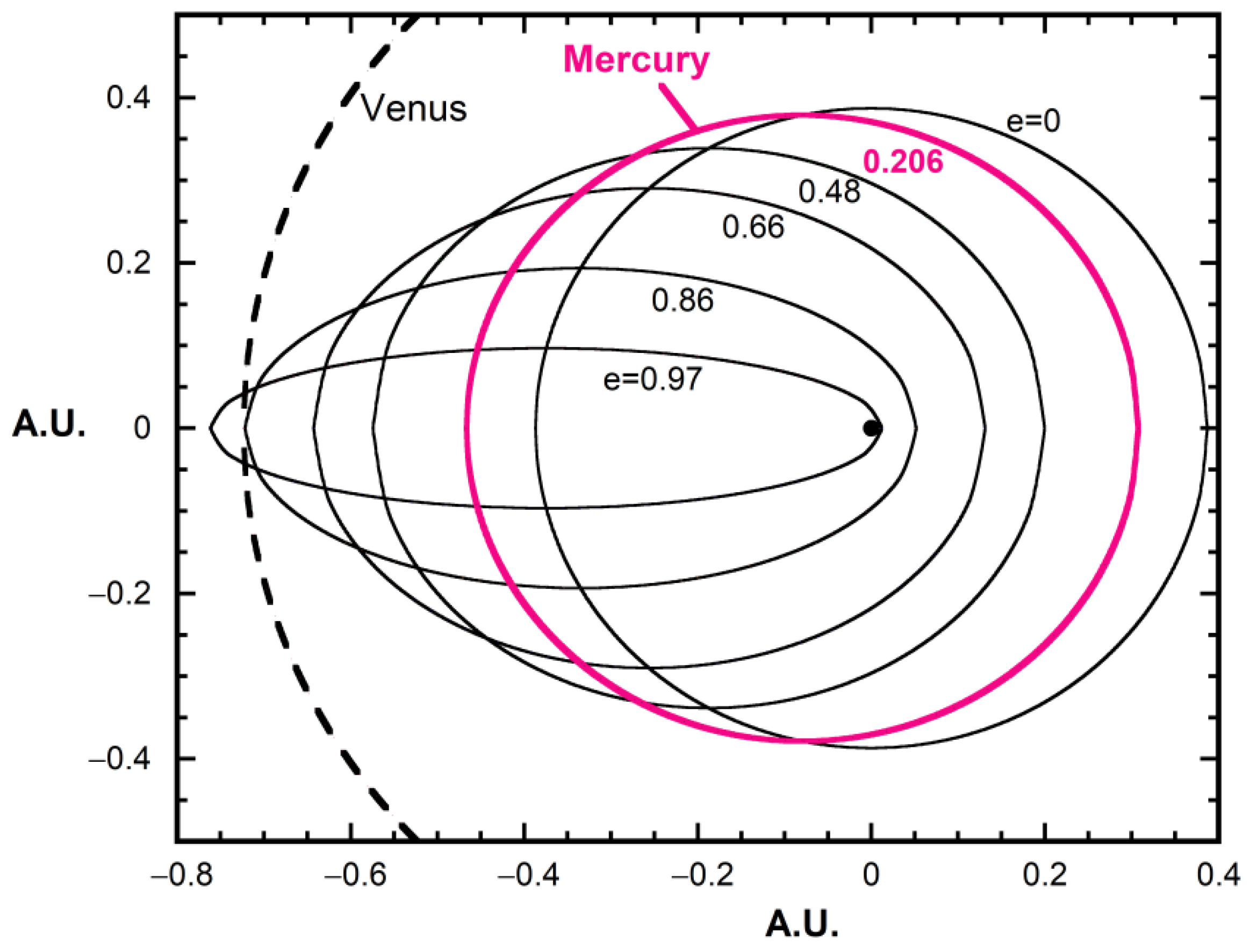
• Orbital eccentricity can change, even under the strong restriction of energy and angular momentum being conserved separately for each closed orbit. This is evident from Equation (4), which is based on the average radius. See [22] for further discussion. Figure 4 shows various possibilities for Mercury.
• Inclinations changing do not affect angular momentum magnitude or energy as this parameter does not enter into the equations for the orbits (Section 2.1). Additionally, any inclination is permitted about the Sun in the Keplerian formulation.

To deduce other possible solutions, and provide details on changing inclinations, we next analyze motions by considering the symmetry of the orbits.

3. Symmetry Constraints on Orbital Evolution Due to Paired Point-Mass Interactions

3.1. Motions Induced by Symmetrical, Small Forces during an Interaction Cycle

Several facets of behavior follow from the forces of Equation (5) reaching only ~10⁻³ times Solar (Equation (2)) and only at the closest passes. Since gravity draws pairs together, their positions are perturbed in opposite directions at any instant. With no frictional forces existing, and these perturbing forces being equal but in opposite directions and changing over the cycle, to first order and a reasonable degree of accuracy, linear momentum along the vector between the pair of planets must be conserved over the cycle. However, observations cannot detect these tiny motions. Instead, efforts are directed to deduce the changes in orbital parameters of Equations (1) and (4) from the apparent motions. Symmetry is extremely useful in this regard, as follows.

Figure 5 illustrates the symmetrical effects of an inboard and outboard planet each on a planet of interest. Relative to the stationary Earth, Venus pulls Earth forward and inward (Figure 5b) upon their close approach because Venus is moving prograde. This situation persists until their furthest separation, after which Venus is pulling Earth in the retrograde direction, but still inwards. However, torque does not exist at the closest and furthest approaches since radius and force vectors are parallel. Furthermore, for a circular orbit of an inboard PP, cancellations of forces describe all other pairings of positions. Thus, torques balance exactly over the circuit, while the outboard POI is pulled inwards. The angular momentum of the POI cannot change over the cycle for circular orbits, and thus neither can the orbital energy.

Conversely, the net effect of an outboard PP over an interaction cycle is to exert an outward force on the inboard POI (Figure 5a), partly due to the inverse square law. Likewise, angular momentum and thus energy are conserved.

From the above:

• On average (i.e., over the cycle), the inboard planet of a pair pulls its outboard partner towards the center. Taken at face value, the outboard planet’s orbital radius could contract over the cycle, and conversely the inboard planet’s radius could expand, in accordance with Newton’s third law. However, these radius changes are inferred in view of introducing a perturbing planet (PP). As the Solar System formed essentially simultaneously, the radius of any given planet already accounts for the presence of inboard and outboard mass. Moreover, the conservation requirements of Section 2.2 cannot be met during radius changes of the pair.
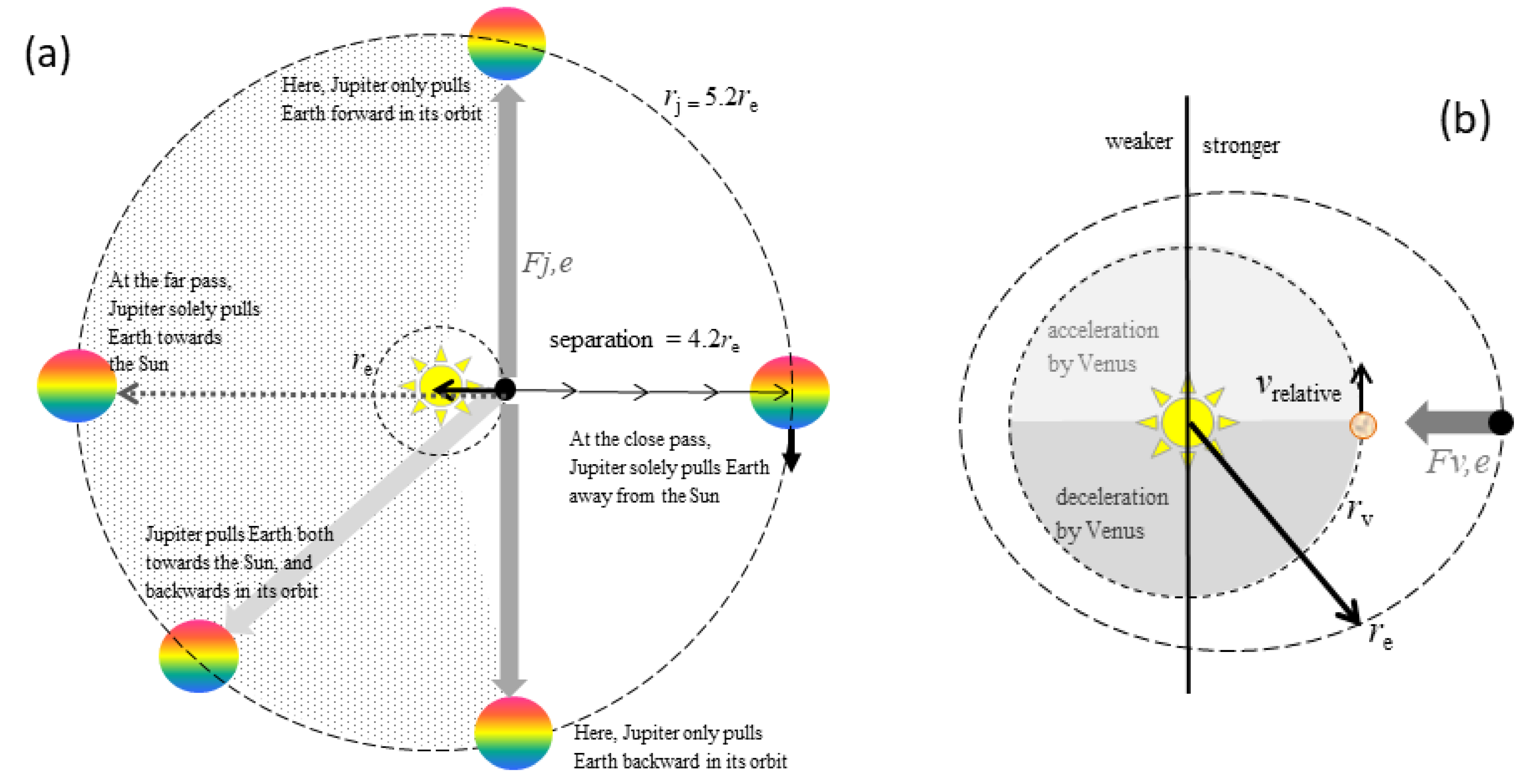
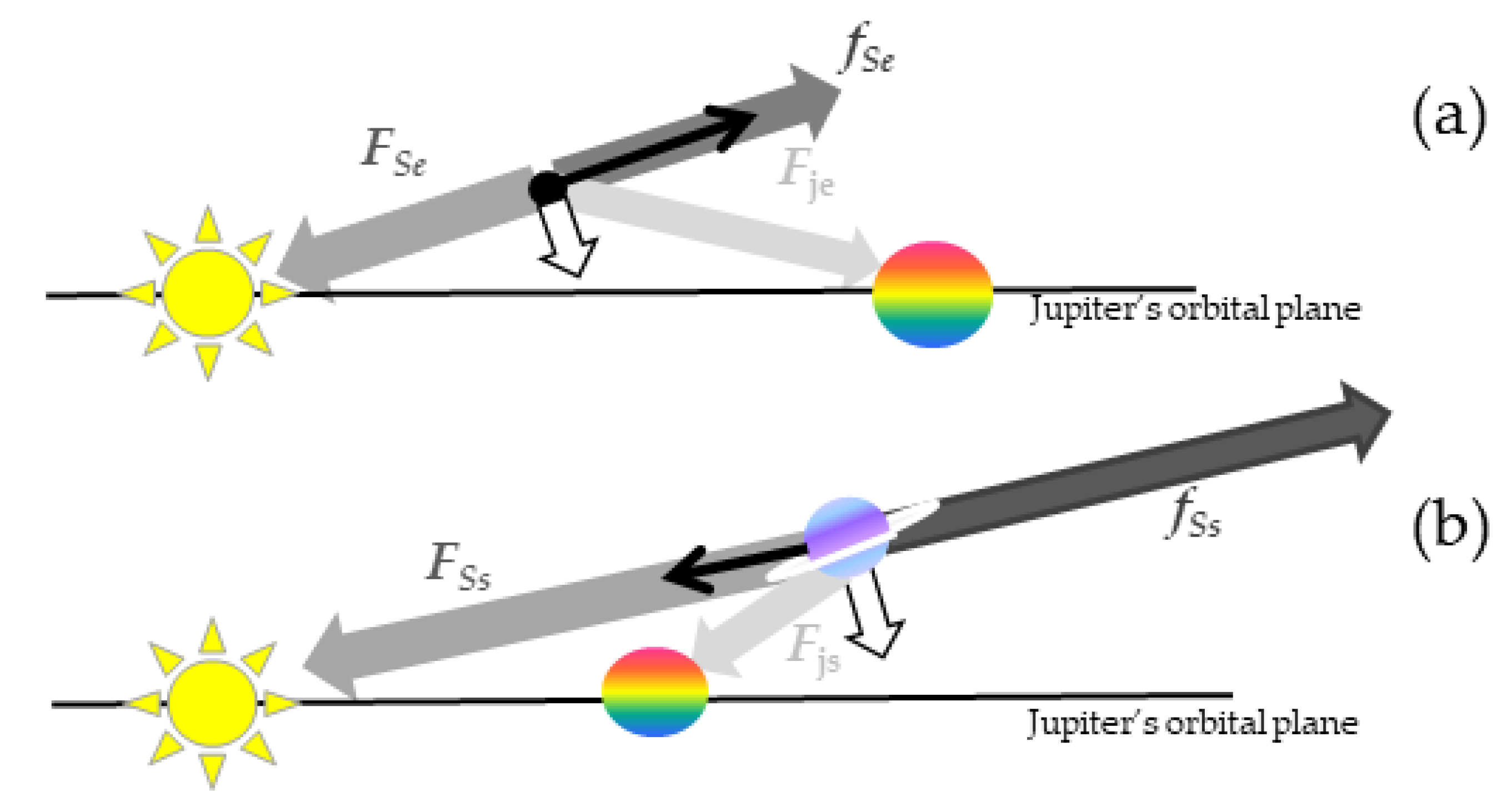
• From the symmetry of circular orbits, the faster inboard planet pulls the slower outboard planet forward, and conversely, but only during one half of the interaction cycle (Figure 5b). The converse holds for the other half cycle. As such, tangential forces should sum to zero over an interaction cycle.
• With small forces, the net change in angular momentum over the cycle is null, i.e., angular momentum should be conserved to first order over the interaction cycle. Precession is thus a second-order term in our analytical perturbation model.
• Because angular momentum is a function of Iω, and energy is a function of Iω², it is not possible to change the energy of an orbit without changing the angular momentum (Iω). Because our model considers only symmetrical perturbations by point-mass interactions, no angular momentum change occurs.
• Changes in eccentricity and inclination angle are permitted (Section 2.2) and thus are the dominant changes.

3.2. Changes in Eccentricity from NIPI and the Effect of Eccentricity on Interactions

Due to balanced torques and consequent conservation of angular momentum, planet–planet interactions increase only eccentricity. From Equation (5) and Figure 5b, Venus in a circular orbit pulls less strongly on Earth at its apogee (depicted) than at its perigee. It is this imbalance that elongates the orbit of an outboard POI. During a close pass with Jupiter (Figure 5a), Earth is pulled out more strongly when it is at its apogee than at its perigee, so an outboard PP also elongates the orbit of its inboard POI. Changes in eccentricity increase with e, so this change is accelerating. Orbits being nearly circular after 4.5 Ga (Figure 3) confirms that NIPI effects are small.

For both geometries, the eccentricity of the POI’s orbit has a small, higher-order effect, due to e being small and the Solar force being strong. Thus, for a pair involving one elliptical and one circular orbit, as considered by Hill [8,9], angular velocities are unchanged over a cycle to a high degree of accuracy. However, the relevant cycle is much longer because the POI must both complete its orbit and line-up with the PP simultaneously. Because the eccentricity is small, paired elliptical orbits behave similar to circular pairs, but the cycle providing the average is huge! Available measurement times (<165 years) cannot gauge this, so our results for changes in orbital radii suffice to describe changes that we might observe.

3.3. Tilted Orbits Are Continually Torqued

Torque exists because planetary orbits are inclined to one another (Figure 3a). During a close approach, a PP pulls a POI towards the orbital plane of the PP, whether the PP is inboard or outboard of the POI (Figure 6). The pull is toward the PP’s plane during far approaches as well, and so this perturbation is unidirectional, although the magnitude of the pull varies during the interaction cycle. Because angular momentum is conserved for the pair, and orientations of the planes are not controlled by Solar forces, the planes of POI and PP move towards each other.

Jupiter is ~300× more massive than the rocky planets (Figure 3b), so its plane is effectively stationary. Jupiter’s strong draw and proximity to the inner planets explains the trend in their inclinations (Figure 3a). The gas giants are ~10× as massive as the ice giants (Figure 3b). Due to trade-offs in proximity and mass, Jupiter and Saturn perturb the ice giants similarly (Figure 7), which explains their inclinations lying between those of Jupiter and Saturn (Figure 3a).

However, quantifying the evolution of inclination requires a theoretical model that incorporates specific positions and motions in tilted planes over a circuit. Such a detailed model is beyond the scope of the present report.

3.4. Summary

Planetary interactions involve accelerations with changing signs, which underscores why assuming steady-state is inappropriate. Radial and tangential accelerations must be described as periodic functions with maxima and minima. For an outboard planet, much stronger forces exist when the PP is close to the POI, than far. Hence, close approaches are important to NIPIs, but forces are greatly reduced as d and a increase (Figure 7). Consequently, the rocky inner planets are little affected by the gas giants, except for Jupiter, due to its large mass and proximity. Interactions between the giant planets seem strong relative to Solar (Figure 7), despite lengthy cycles (Figure 1 and Figure 2; Table 1).

An outboard planet causes the orbit of an inboard planet to expand, with respect to the Sun alone, but does not change its angular velocity to first order. Hence, perihelion of the inboard planet can advance as a second-order perturbation because POI tangential velocity is too large for its new position. From symmetry, the converse holds for the outboard planet. Many of the signs for precession listed by Dolittle [10], who used Hill’s [8,9] ring model, are inconsistent with this analysis. Magnitudes necessarily err: even if the planets were shaped like rings, central forces do not describe the pull of a ring [14]. Possibly Gauss [7] had misgivings about the ring construction, as he never completed his analysis.

4. Numerical Models of Newtonian Interplanetary Point-Mass Interactions

4.1. Numerical Methods

Most orbits have semi-minor and major axes differing by less than 0.4% (Figure 3b). To construct our numerical model, all orbits are depicted as circular. Measured masses, average orbital radii (a), and the consequent periods [15] are used as inputs in calculating tangential and radial accelerations. Forces are calculated assuming steady-state orbits and velocities, appropriate over the time periods explored.

Each calculation models the effects of two perturbing planets, which act independently of each other, and of the Sun on one planet of interest. The starting position is co-linear. Planet positions were calculated using a 0.1 day time step. At every step, Newton’s law was used to calculate the force of each PP on the POI, and the force of the Sun on each planet. Radial and tangential forces were calculated for each planet. The results are presented as accelerations of the POI relative to that of the Sun, which are equivalent to force ratios. These two accelerations drive evolutionary changes in orbits.

Calculations were pushed forward ~10,000 days. Because orbits are exactly circular, they repeat somewhat frequently, so using ~10,000 days in our calculations should suffice to establish the average accelerations for the pairings. Only the pairings of the three outermost planets have interaction cycles longer than ~27 years (~9862 days). Although the 0.1 day step time prevents the algorithm from exactly capturing the symmetry of the modeled circular system, many interaction cycles are sufficiently large (e.g., 820 days describes Jupiter and the closer planets) that the results should be reasonably accurate. The calculations describe the perturbations of the present-day system over a short interval compared to geologic time, but one that should represent observational data, which are limited to durations <165 years.

4.2. Perturbation of Mercury by Outboard Planets in Circular Orbits

Accelerations of Mercury both along and perpendicular to its orbit are periodic. Jupiter encircles the Sun sufficiently slowly compared with Mercury that this interaction duration nearly equals the orbital period of the POI (Figure 8a). Tangential and radial accelerations of Mercury by Jupiter somewhat resemble sinusoidal curves. The action of Venus on Mercury has a longer period of 144.5 days (or 0.395 y = 1.64 orbits of Mercury), which differs slightly from the orrery estimate in Table 1, because the latter includes Mercury’s orbital eccentricity. The actions of near-by Venus consist of long intervals of weak radial deceleration that are punctuated by an acceleration peak centered on each close pass. This peak has a roughly Gaussian shape. The tangential accelerations somewhat resemble a derivative of the radial accelerations by Venus.

Extrema in the radial accelerations on Mercury computed from Equation (5), and normalized to Equation (2), agree with our numerical results, as indicated in Figure 8.

Tangential accelerations average to ~0 over an interaction cycle of the POI with the PP (Figure 8a), confirming findings in Section 3. The balance occurs over neither the orbital period of the POI nor over a Julian year. In contrast, radial accelerations are positive over an interaction cycle. The averages of the numerical models (heavy lines) are lower than simply averaging the extrema (dotted lines and open symbols), where the difference is smaller for the action of Jupiter due to its roughly sinusoidal action on Mercury. Jupiter and Venus similarly perturb Mercury over their respective interaction cycles.

Calculated accelerations of Mercury both along and perpendicular to its orbit become more symmetrical as the distance of the PP from the POI increases: compare Figure 8b for the effects of Earth and Saturn to Figure 8a for the effects of Venus and Jupiter, respectively. Amplitudes decrease in agreement with Equation (5). The increasing symmetry with distance moves both extrema averages and averages with time towards zero. Weak actions of low mass Mars, or distant Neptune and Uranus, on Mercury (Figure 7) can therefore be neglected.

Positive net radial acceleration does not indicate that Mercury is moving outward. The average pull to the center is balanced by the average centrifugal forces of the orbit. Rather, the presence of a PP increases the eccentricity of an orbit, which is permissible, and in a rather complicated fashion.

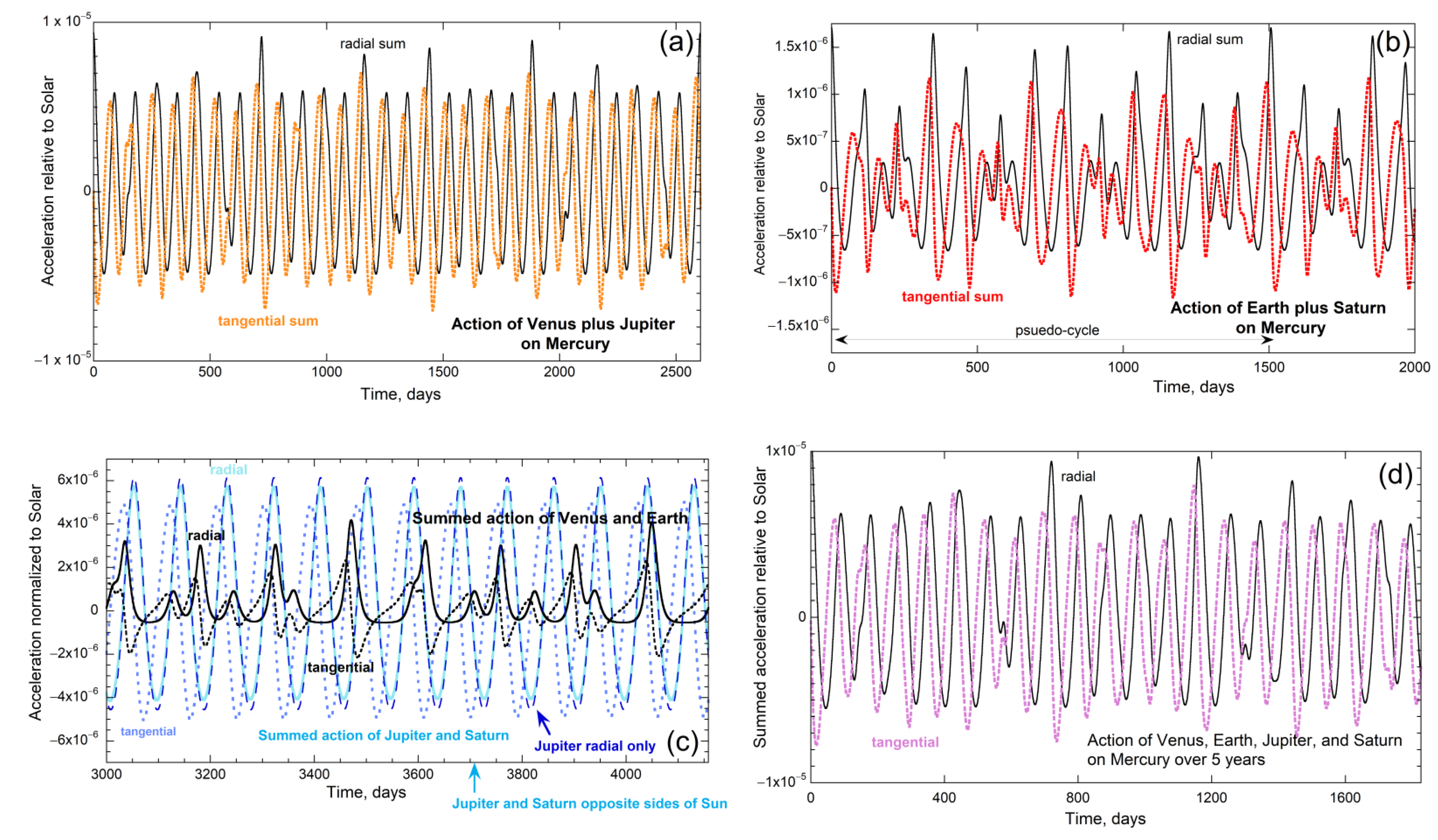
4.3. Sums of NIPI for Mercury Reveal Beat Patterns

The sum of the two strongest perturbations from Venus and Jupiter on Mercury (Figure 9a) is dominated by the interaction cycle with Jupiter at ~88 days, yet the excursions in accelerations are enhanced by the draw of Venus. Their summed action has a very long cycle of 8529.3 days, although after 2603 days, the planets are close to the initial collinear configuration.

Table 2. Average accelerations (relative to Solar) as a function of interval from numerical models of the actions on Mercury, which has an orbital period of 87.97 days.

Perturbers	Interval Days	Significance	No. Orbits	Average Acceleration Ratios
				Radial *	Tangential
Venus + Jupiter	2604	pseudo-cycle †	29.6	4.6985 × 10−7	−1.60 × 10−10
	3652.5	10 Julian years	41.5	4.5812 × 10−7	−4.23 × 10−8
	7305	20 Julian years	83.0	4.7779 × 10−7	−2.35 × 10−8
	8529.3	complete cycle	96.9	4.6986 × 10−7	−2.26 × 10−11 ‡
Earth + Saturn	1507	pseudo-cycle †	15.7	1.1422 × 10−7	−2.15 × 10−11
	3652.5	10 Julian years	41.5	1.1483 × 10−7	−5.11 × 10−9
	7305	20 Julian years	83.0	1.1529 × 10−7	−1.67 × 10−9
	7184.3	complete cycle	81.6	1.1395 × 10−7	−6.89 × 10−13 ‡
All §	3652.5	10 Julian years	41.5	5.741 × 10−7	−4.934 × 10−8 §
	7305	20 Julian years	83.0	5.930 × 10−7	−2.522 × 10−8 §

* Positive radial acceleration increases the radius. † The pseudo-cycle is defined by the pattern of cycling in Figure 9, but closely examining the data showed that the planets were not exactly co-linear as in the starting configuration. ‡ This low value is null, within uncertainty of the calculation. § Neither a pseudo-cycle nor a full cycle was indicated over the 24 years probed, and so the tangential acceleration is not representative. These four PPs describe the total action, since accelerations from Mars, Uranus, and Neptune are low and similar to calculation uncertainties.

lists averages computed over various intervals. The interval selected strongly affects the average tangential acceleration, but weakly affects the average radial acceleration. For arbitrarily selected intervals such as 10 Earth orbits, the tangential acceleration resembles the average of the radial component, even though its true average is negligibly small.

The summed actions of Earth and Saturn on Mercury (Figure 9b; Table 2) behave similarly. Saturn controls the beat, whereas Earth enhances the excursions. Due to the high symmetry of Saturn’s periodic action, its true and pseudo-cycles with Earth are shorter than those of Venus combined with Jupiter on Mercury (cf. Figure 9a,b). Choosing intervals different from an interaction cycle yields erroneous tangential averages. We infer that precession determined from modeling observational data is a consequence of using Julian years, not interaction cycles.

Summing accelerations from Jupiter and Saturn (Figure 9c) shows that distant PPs together provide roughly canceling accelerations and decelerations at intervals comparable to the orbital period of Mercury. Summed accelerations of Venus and Earth provide spurts of strong accelerations in a lop-sided pattern that repeats every 577 days. Clearly, the beat patterns in a four-body system depend on PP distance.

Summing accelerations of Venus, Earth, Jupiter, and Saturn on Mercury (Figure 9d) depicts the entire effect of the Solar System, since Mars is small while Uranus and Neptune are distant. The pattern does not repeat within ~24 years. For circular orbits, returning to close to the initial configuration probably requires ~460 years, which is a consequence of the very different NIPI cycles (Table 1; Figure 8 and Figure 9). Our numerical calculations show that the tangential acceleration of Mercury is null on average, even if the duration of the full interaction cycle is not known.

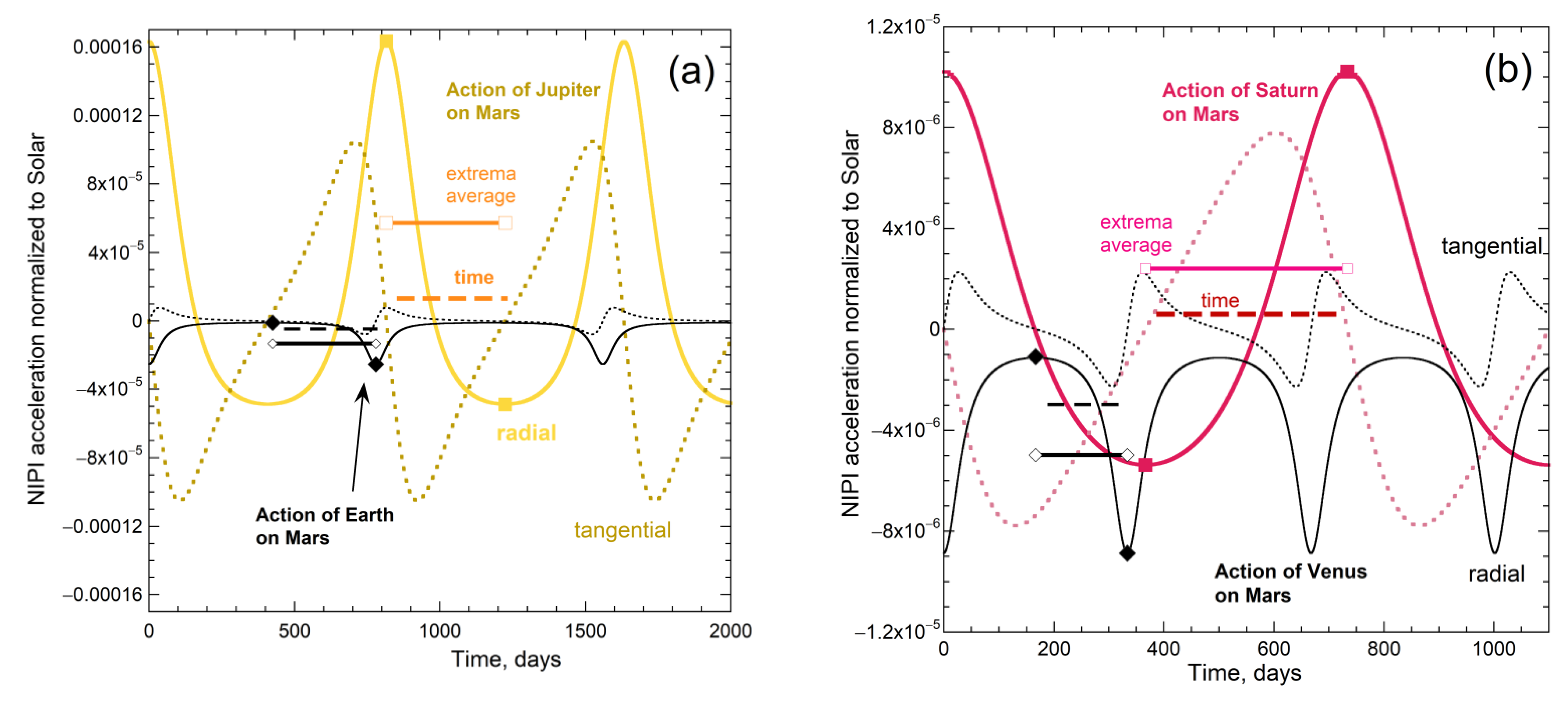
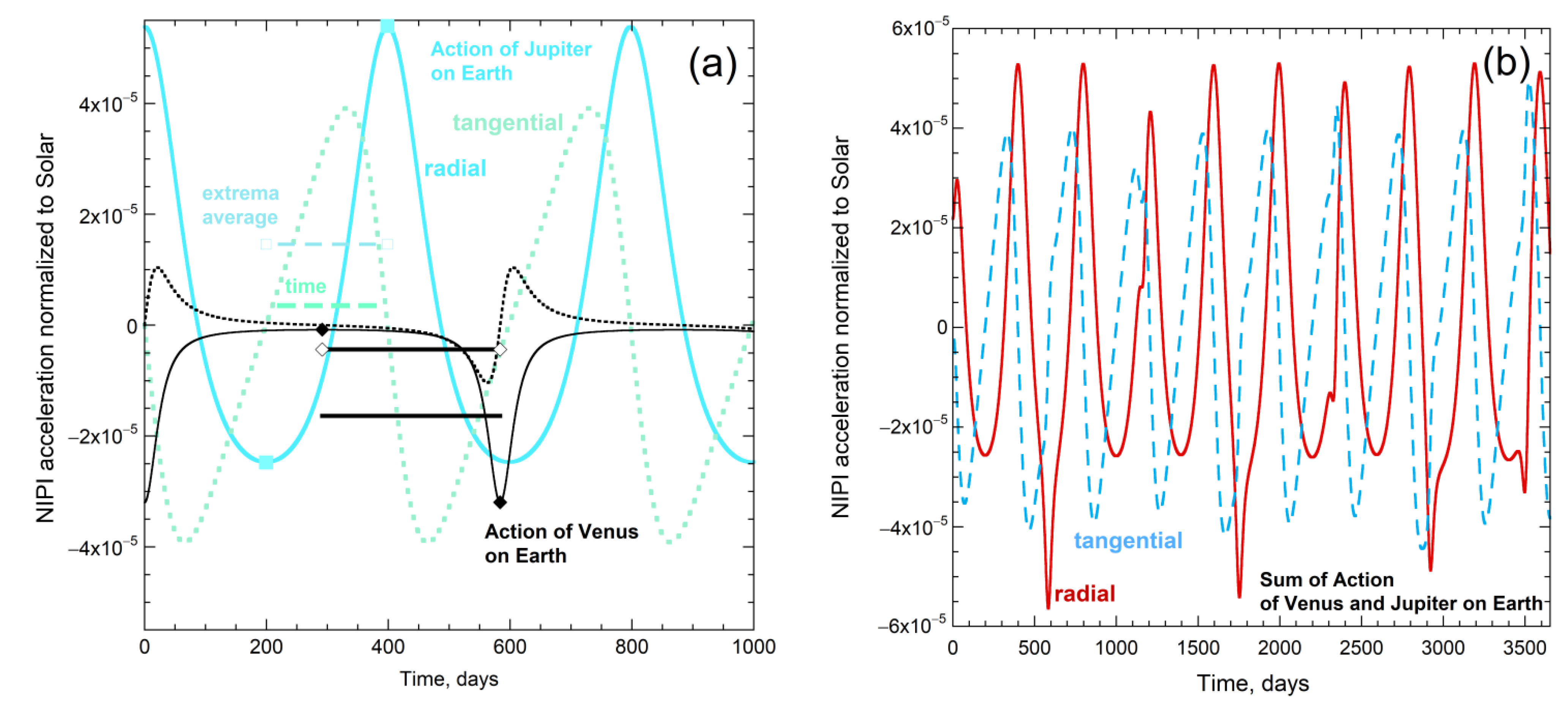
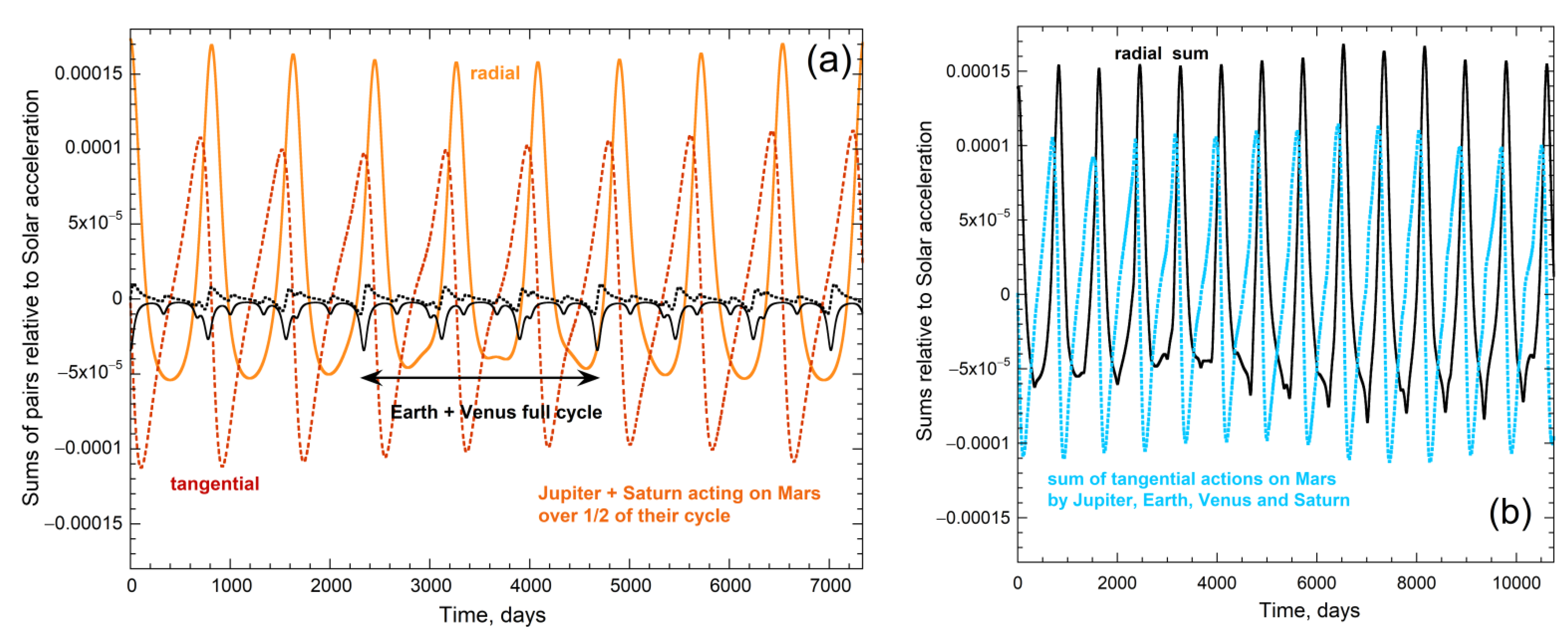
4.4. Competition of Inboard vs. Outboard PP Actions on Mars and on Earth

Outboard Jupiter provides the strongest perturbation on Mars. This pattern (Figure 10a) has a similar shape as the actions of outboard Venus (or Earth) on Mercury (Figure 8), where the segment of low radial deceleration is a broad valley rather than being rather flat. The acceleration peaks are quite high. Inboard Earth always pulls Mars inward (Figure 10a), such that strong peaks are separated with wide flat zones of weaker inwards pull. Compared to Jupiter, Saturn provides more rounded regions of deceleration and lower peak heights, so the overall shape is more sinusoidal (Figure 10b). Compared to Earth’s effect, more distant inboard Venus provides narrower flat decelerations (cf. Figure 10a,b).

Figure 11a shows the two strongest perturbations on Earth. Jupiter acts on Earth similar to its action on Mars (Figure 12), but the peak acceleration is weaker. Venus always accelerates Earth inward, with a flat weak deceleration and strong negative peaks.

Although the maxima and minima are affected strongly by the mass and distance, the pattern for the radial acceleration with time is determined solely by the position of the PP (inboard or outboard), where the shape is stretched or compressed in time depending on the separation of the two bodies. As the distance increases to an outboard PP, the radial acceleration becomes more sinusoidal in appearance. As the distance increases to an inboard PP, the negative radial peaks become more closely spaced.

Tangential accelerations average to zero over appropriate cycles, regardless of the position of the PP relative to the POI. In agreement with Section 3, the first-order consequence of NIPI is to perturb orbital radii, compared with the radii when the PP is not present. Therefore,

Table 3. Numerical determinations of average radial accelerations relative to Solar.

POI	PP	Time Average *	Extrema Average *	Ratio
Mercury	Venus	0.2735	1.473	5.38
	Earth	0.1047	0.483	4.61
	Jupiter	0.1967	0.794	4.40
	Saturn	0.00832	0.0375	4.50
	Sum ‡	0.583	2.79	4.8
Venus	Mercury	−0.065	−0.419	6.4
	Earth	2.81	9.99	3.56
	Mars	0.088	0.111	1.26
	Jupiter	1.3 §	5.33	4.3 §
	Saturn	0.057 §	0.25	4.3 §
	Sum ‡	est.5.5	15.26	est. 2.8
Earth	Mercury	−0.038	−0.18	4.66
	Venus	−4.38	−16.4	3.74
	Mars	0.215	0.540	2.50
	Jupiter	3.52	14.6	4.14
	Saturn	0.15 ‖	0.665	4.4 ‖
	Sum ‡	−0.86	−1.80	2.1
Mars	Venus	−2.97	−4.98	1.68
	Earth	−4.65	−13.3	2.86
	Jupiter	13.2	57.2	4.3
	Saturn	0.591	2.42	4.1
	Sum ‡	6.17	41.3	6.7

* Accelerations should be multiplied by 10⁻⁶. The averages sum because the actions are independent, regardless of the precise cycle length. ‡ This sum represents all planets, since the effects of Uranus and Neptune are negligible. Values from combining Equations (2) and (5), which are exact instantaneously. § Estimated from the assumed ratio of 4.3 in the rightmost column, which is based on the averages for the extrema and numerical calculations for the action of Jupiter and/or Saturn on Mercury, Earth, and Mars. ‖ Estimated from the action of Jupiter on Earth, based on actions of Saturn relative to that of Jupiter on Mercury and Mars.

reports radial averages for the paired interactions.

4.5. Sums Involving Inboard and Outboard PP

For Earth and Mars, as calculated for Mercury, cycles with more than one planet can be very long and are not multiples of Julian years (Figure 11b and Figure 12). Uranus and Neptune are not discussed because their impact is negligible, due to distance. The impact of Mercury is also tiny, due to its low mass, and is likewise neglected.

Summing the action of both outboard giants on Mars (Figure 12a) yields a beat pattern with a period near 816 days, which stems from the action of Jupiter (Figure 10a), which repeats every 821 days from our estimate (Table 1) based on Ford’s [3] orrery (Figure 6). The true cycle for the combined action is 7347 days.

Summing the action of the largest inboard planets on Mars gives a fairly short cycle (2339.2 days) of deceleration where the close passes provide jerks (Figure 12a). Accounting for Mercury would add tiny deceleration peaks.

The sum of these four neighboring PPs (Figure 12b) represents the action of the entire Solar System on Mars. Even with assuming circular orbits, calculations over ~24 years did not yield information on a true cycle or even a pseudo-cycle.

Regarding Earth, summing the actions of Venus and Jupiter yields a long pseudo-cycle of 8792 days (Figure 10b). Jupiter creates the beat pattern, while Venus provides the strong inward accelerations.

Averaging the extrema for the actions of all planets on Earth, computed from Equations (2) and (5), shows that Venus and Jupiter dominate NIPI perturbations of Earth (Table 3). Because interactions consist of coupled pairs, we estimate the time average for the small action of Mars on Earth from the numerical calculation of the time-averaged action of Earth on Mars, again using Equations (2) and (5). This use of symmetry gives a time-average consistent with the calculated averages for other interactions. The same holds for the time-average likewise estimated for the effect of Mercury on Earth (Table 3). The action of Saturn on Earth was estimated from the action of Jupiter on Earth, based on the action of Saturn, relative to that of Jupiter, on Mercury and on Mars. This estimate is supported by the ratios of extrema and time averages all being 4.1 to 4.5 regarding actions of the gas giants on the rocky planets (Table 3).

Average radial accelerations were similarly estimated for Venus from its action on other rocky planets and from the regular behavior of the actions of Jupiter and Saturn on the inner Solar System. Venus is pulled outward, due to the combined effects of Earth and Jupiter, but not so strongly as Mars.

5. Discussion

5.1. Consistency of Numerical Results for Accelerations with Geometrical Analyses

The results of our numerical calculations of planetary perturbations on circular orbits (Figure 8, Figure 9, Figure 10, Figure 11 and Figure 12; Table 2 and Table 3) confirm that tangential forces balance over the interaction cycles affecting any given POI, which was inferred from symmetry and asymmetry of the forces and torques over an interaction cycle (Figure 4). To acceptable accuracy, torque does not exist over the interaction cycle, so the angular momentum of each planet is conserved cyclically.

The numerical results also confirm that the net (average) acceleration in the radial direction is positive (away from the Sun) when the PP is outboard of the POI. When the PP is inboard of the POI, the converse holds. These net accelerations from geometry (Figure 4) or the calculations (Figure 8, Figure 9, Figure 10, Figure 11 and Figure 12) are relative to the two-body Sun–POI system, whereby radial forces are balanced by centrifugal accelerations at every instant. Our results suggest:

• The existence of a perturbing planet changes the perpetual balance of radial pull with centrifugal acceleration of the two-body solution for the POI to a balance over its interaction cycle with the PP.
• These interaction cycles of the three-body subsystems are fairly long (Table 1), but are tiny compared to cycles involving more than one PP (Figure 8, Figure 9, Figure 10, Figure 11 and Figure 12).

5.2. Permissible Changes in Orbital Parameters

Conservation of angular momentum is compatible with the rotational kinetic energy of each planet being unchanged over an interaction cycle (Section 2.2 and Section 3.1). Only eccentricity and inclination can change.

The radial force exerted by a POI elongates the orbit of the PP. Elongation of Mercury’s orbit is shown in Figure 4, but from symmetry, the orbit of the outboard planet is also affected. The relative masses of the two planets and conservation of linear momentum of the pair determine the extent of the elongation, and which planet of the pair is most affected. As Mercury is tiny, the other planets are negligibly affected (Figure 7).

Our results on tangential accelerations indicate that precession of perihelia is miniscule. Importantly, the average radius, which equals the semi-major axis, is unchanged. Inclination can change because this variable defines the plane of the orbit, not the orbit itself.

5.3. Comparison of Model Results with Deduced Basic Orbital Parameters

That conservation laws are upheld is evidenced by the observations. Foremost, orbits are impressively close to simple, stable Keplerian ellipses. The present-day Solar System does not possess large radial velocities. Precession of perihelia seems to have been detected by Newcomb [23] and values have changed little since then [1,11], but are these precession values reliable? Are these models of observational data actually showing net changes in tangential velocity?

Seven planets are an insufficient number to “average out” the cycles. Our numerical models show that periodicity of the interactions is very important to each and every planet. It is long accepted that such periodicity affects the gas giants, as is evident from orrery visualizations (Figure 1). Consequently, any average needs to be computed over an appropriate interval (Table 1). However, even long intervals are insufficient to produce a valid average, due to the “resetting” of the both radial and tangential accelerations to zero up to twice each cycle of any given pair, depending on whether the PP is inboard or outboard. Rather, the duration must match the interaction cycle of any given POI, which depends on all its interactions. Furthermore, because interaction cycles differ from orbital periods (Table 1), observations based on Earth-years are not germane.

Clemence [24] used 100 Earth years to survey Mercury. The period used by Simon et al. [1] to analyze each of the eight planets is unclear because the basis was several datasets collected over various intervals (~6 to 165 years, with an emphasis on ~65 years of optical data and ~10 years of radar data, per the discussion of Standish [25]). The observations are not recording a properly averaged tangential acceleration, and thus misrepresent precession of orbital perihelia.

For three interacting planets, full interaction cycles are very long, exceeding decades (Figure 8, Figure 10, and Figure 11). For the actions of four planets on Mercury or on Mars, cycles reach centuries, from extrapolation of our results. Hence, astronomical measurements of the bodies against the stars and/or with reference to the Sun are probing the various boosts and brakes, but not evolutionary behavior. Thus, the time dependence has not been ascertained for any planetary orbital parameters from astronomical measurements. Simply put, Solar system dynamics cannot be ascertained from a mere ~165 years of astronomical measurements due to the complex, yet symmetric, interactions.

5.4. Inclinations and Evolution

Inclination can change because out-of-plane triangular configurations in a three-body system provide torque (Figure 7; Section 3.3). Presently, Uranus and Neptune occupy the plane intermediate to Jupiter and Saturn. Inclinations of the rocky planet relative to Jupiter decrease as Jupiter is approached; these data in Figure 3a are fit by:

i (in degrees) = 8.4517 × 10¹⁸ a^−1.6869,

(6)

where a is in meters. The simplicity of Equation (6) supports the process of torque described in Section 3.3, where the evolution of the small bodies near Jupiter has been towards its plane. Pairwise conservation of angular momentum perpendicular to the plane of the pair exists, while depending on relative planetary masses (Figure 3b and Figure 7).

Confidently estimating the rate of change of inclination with time is difficult. The rate depends on the initial inclination, which is unclear. Interestingly, Uranus’ spin axis is perpendicular to its orbital axis, unlike all other planets, which spin nearly upright with the same sense as their orbital motion. The unique configuration of Uranus can be explained if Uranus formed in a near-polar orbit, as has been observed for dwarf satellite galaxies encircling Andromeda (see [6] and references therein). After planet formation, Uranus was subsequently torqued by Jupiter and possibly the other planets, which likely had similar orientations to Jupiter, given their spin orientations. The maximum rate of change suggested from Uranus is di/dt < 2 × 10⁻⁸ °y⁻¹, which is tiny, and therefore is consistent with a small perturbation.

Inclination changes will also be affected by interaction cycles. Hence, observations are not detecting evolution of orbital inclinations, but rather are probing the intermittent torques, caused by configurations varying as the planets orbit the Sun (Figure 4 and Figure 7). Although quantification is beyond the scope of this report, the inclinations of all other planets should change more slowly than Uranus, estimated above.

5.5. Eccentricity and Evolution

Force differences, exemplified by those between the close and far passes, elongate planetary orbits. Our model does not quantify the time change. However, the starting point can be no smaller than e = 0, so e increases with time. Since the focus moves further from the center as e increases, de/dt increases with e, as is evident from comparing the configurations in Figure 4 and Figure 5. Data on the present-day Solar System (Figure 3) support these findings, in view of the numerical computations (Section 4), and conservation of linear momentum. The derivatives are very small (

Table 4. Changes in eccentricity, assuming e = 0 at formation.

Inner Planets	Maximum de/dt (Century−1)	Outer Planets	Maximum de/dt (Century−1)
Mercury	4.5256 × 10−9	Jupiter	1.0764 × 10−9
Venus	1.4748 × 10−10	Saturn	1.2437 × 10−9
Earth	3.6760 × 10−10	Uranus	1.0280 × 10−9
Mars	2.0581 × 10−9	Neptune	2.4873 × 10−10

) and cannot be resolved in ~165 years of observation.

The following stems from momentum conservation:

• If the pair is composed of a very heavy and a very light planet, the light planet is displaced far more during the elongation.
• If the masses are equal, no elongation is expected. Rather, the planets approach and recede from their center of mass in a balanced fashion.
• From the patterns of radial acceleration (Figure 8, Figure 9, Figure 10, Figure 11 and Figure 12) for a greatly separated pair, the action of the outboard PP approaches sinusoidal, so the inboard POI oscillates in its orbit, rather than elongation occurring. Due to symmetry, the same holds for its partner.

Mercury having the most eccentric orbit (Figure 3) is consistent with our model: Mercury is both the innermost and least massive planet, so all other planets elongate its orbit, although Uranus and Neptune are too far to be effective. Strong forces arising from its nearest neighbors, Venus and Earth, and from the most massive planet, Jupiter, which is also reasonably close, are the source of elongation.

The orbit of Mars, which is the second least massive planet (Figure 3b), is the next most eccentric (Figure 3a). Jupiter strongly accelerates Mars due to proximity and its huge mass (Figure 10 and Figure 12). The huge mass difference, in view of linear momentum conservation, means that Mars, not Jupiter, is perturbed.

Venus and Earth are the next in mass, and moreover have nearly identical values. These are close and strongly interact. Their next nearest neighbors are the lightweights, which have little effect. Both Venus and Earth have nearly circular orbits because their masses are nearly the same. However, Earth is considerably closer to Jupiter, and so the barycenter orbit has been slightly elongated over history, but not much.

Planets in the outer Solar System are only affected by each other due to their great distances from the rocky planets, which are much lighter. Except for outermost Neptune, the eccentricities are similar. Neptune has a round orbit because it is not only quite distant from massive Jupiter and Saturn, so their effects are small, but moreover its nearest neighbor (Uranus) has a similar mass (Figure 3) and so its effect on elongation is tiny. Conversely, Neptune is ineffectual at elongating the orbit of Uranus due to linear momentum conservation, and ineffective at elongating orbits of the gas giants due to their large masses and great distances. Hence, our model points to perturbations in the outer Solar System involving interactions of Jupiter, Saturn, and Uranus, and is consistent with Neptune being negligibly perturbed over its full interaction cycle.

Uranus is perturbed by the gas giants because of their large mass, but the effect of Jupiter on its eccentricity is fairly low due to the great distance. Conversely, Uranus has little effect on Jupiter.

The gas giants are a pair, but the disparate masses cause the eccentricity of Saturn’s orbit to be greater. Saturn is also more affected by Uranus than Jupiter is due to mass and distance combined. Hence, Saturn has the largest eccentricity in the outer Solar System.

The eccentricity of Jupiter’s orbit is mostly attributable to the action of Saturn, but our model suggests that little elongation is expected. Their interaction period being close to multiples of their orbital periods (Table 1) may have some effect. Another consideration is that Jupiter is being pulled outwards by all other giant planets, relative to the Jupiter–Sun-only orbit. A detailed study is needed of these cyclic interactions, which includes the current orbital eccentricities, to explore actions on Jupiter.

5.6. Precession of the Spinning Earth

The total precession of Earth is determined from the motion of the Sun against the stars (e.g., [26]). The reference plane is the ecliptic, which is based on the fixed point of Earth’s equinox, but otherwise involves an average position for the Sun. Earth’s motions in space are complicated, being described as an axis for the barycenter orbital plane, another axis for the plane of the Earth and Moon about the barycenter, and a third axis of spin through the geocenter (see the figure in Sobchak [27]). Total precession measured against the Polar stars is related to time variations of all three axes. The largest NIPI contributions to Earth from Venus and Jupiter have different signs but similar magnitudes, which reduces the effect of cycle mismatch. Thus, the spin axis is probably the most important, but the wobbling of the axes describing the Earth–Moon plane cannot be neglected. The tilted lunar plane leads to many superimposed cycles: the Saros (~18 years), the Metonic (~19 years), and several much longer cycles [28,29,30]. Moreover, Earth’s year divides unevenly by Earth’s day. Hence, making telescopic observations yearly at the exactly same location in space is impossible.

Existing values for precession are thus imprecise. Morgan [26] obtained a total of 6184″cy⁻¹ from the data. Simon et al. [1] subtracted the historic lunisolar model value from his analysis. Adding this back in gives a total precession of 6190″cy⁻¹. The difference between the 1945 and 1994 analyses of Earth’s precession is thus insignificant.

Precession of Earth’s spin axis as ~6200″cy⁻¹ is reasonable, given data on the pole star. Calculations of Newton circa 1700, who depicted the orbiting Moon as a ring, which is problematic since the force is not central, yielded ~5000″cy⁻¹. Subsequently, the Earth and Moon were modeled as orbiting in a fixed plane, yielding a similar number by many authors. Neither configuration describes Earth’s complex orbit [27]. The historic lunisolar models warrant revisiting.

6. Conclusions and Implications

Foremost, interactions among pairs of planets are decidedly periodic (Table 1). Because planet masses are tiny compared to the Sun’s, the perturbing forces are small. Hence, the interactions can be modeled using circular orbits. The planets give each other boosts and brakes, in a cyclical fashion, which stems from the overarching control of the orbits by the more massive Sun. Without friction, energy and momentum are conserved over the various interaction cycles in the three-body sub-systems. Multi-planet behavior differs from that of two-body systems, where accelerations inward and centrifugally balance at all times. However, any effect on any given planet changes the entire Solar System. Hence, the current configuration of the eight largest bodies in the Solar System largely recapitulates the initial arrangement, essentially due to “gridlock”.

We have shown that angular velocities and the semi-major axes are constant over interaction cycles. Hence, only eccentricities of the orbits and inclinations of the orbital planes are evolving with time. These data are consistent with the mass and distance between the various planet pairs, except possibly for Jupiter’s orbital eccentricity being fairly large, i.e., approaching that of Uranus. However, Jupiter is perturbed by three large outboard PPs, and the changes are accelerating.

The period associated with NIPI interactions differs from the orbital period of each planet of interest, especially for adjacent perturbing planets (Table 1), which commonly have the greatest influence (Table 2, and several figures). In addition, the sum of NIPI interactions has a very long period because orbits are unsynchronized, and periods do not share a common denominator. Consequently, observational measurements made from the Earth and in reference to the equinox and Earth-years do not correspond to NIPI cycles, even for the Earth and even if its actual orbit were Keplerian. Although perihelia precession of the planets seems to exist with reference to the background of stars, this does not represent evolutionary behavior, but instead is a result of Julian measurement intervals being disconnected from interaction cycles.

As such, planetary orbits are incrementally variable orbits dominated by periodic behavior. For forecasts over short time periods, periodic approximations are usually sufficient; however, the long-term behavior of the system will not be captured correctly by these approximations. Perfectly periodic behavior differs fundamentally from aperiodic responses, and periodic equations can never correctly capture irregularity. Yet, the nearly Keplerian orbits indicate that 4.5 Ga is insufficient to reach aperiodic responses, except possibly for Jupiter.

Implications are far from trivial. Our understanding of graviation largely traces to planetary observations. Historical acceptance of general relativity stemmed from Clemence’s [11] use of Hill’s [8,9] ring model, as applied by Dolittle [10]. Fortuitous agreement with observations was obtained, as a consequence of the incorrect sign and magnitude for the summed model perturbations, and because not all components of the Earth’s precession were included in the evaluation (Section 5.6). Precession of the axis of the Earth-Moon plane is unaccounted for today. It is not currently possible to evaluate the relativistic models for Mercury due to the NIPI cycles differing from durations of observations, as well as to uncertainties in the theory of Earth’s luni-solar precession.

The Virial theorem of Clausius applies, which is a consequence of linear momentum cancelling in all directions over the restricted space that defines any given bound state [21]. The Solar System is a bound state. Importantly, the Virial theorem is independent of conservation of energy; these constraints together greatly restrict orbital characteristics and dynamical behavior. However, as shown in Figure 4, over a long time Mercury’s orbit will evolve towards permitting collisions with Venus. Before this, the action of Venus on Mercury will increase to the point that it is no longer a perturbation compared with the Solar force. At some point, Mercury, Venus, and the Sun will constitute a three-body problem. For the interesting situation of high eccentricity and strong accelerations, a different approach than the present perturbation model is needed.

To summarize, our key findings are:

• Hill’s steady-state ring model is inapplicable.
• Observational data are not only influenced by the geocenter’s peculiar orbital path around the Sun, but more importantly represent incomplete cycles of interplanetary interactions.
• Mercury’s orbit is Keplerian, within the uncertainties of short-term observational data. Adding a relativistic correction is not supported by the existing data. Such corrections should be applied only after observational data are corrected for Earth’s non-Keplerian orbit, and precession models based on transient planetary interactions are considered.
• Conservation laws and the Virial theorem set stringent limits on the evolutionary behavior of the eight planets. Only eccentricity and inclination can change, as long as the interplanetary forces are small compared with Solar (<2%), which is met today.
• The pair Jupiter–Saturn merits closer examination, as these are the most strongly interacting planets.

References

1. Simon, J.L.; Bretagnon, P.; Chapront, J.; Chapront-Touze, M.; Francou, G.; Laskar, J. Numerical expressions for precession formulae and mean elements for the Moon and the planets. Astron. Astrophys. 1994, 282, 663–683. [Google Scholar]
2. Chapront, M.; Chapront-Touzé, M.; Francou, G. A new determination of lunar orbital parameters, precession constant and tidal acceleration from LLR measurements. Astron. Astrophys. 2002, 387, 700–709. [Google Scholar] [CrossRef] [Green Version]
3. Ford, D. Solar System Orrery. Available online: https://in-the-sky.org/solarsystem.php (accessed on 15 July 2018).
4. Hofmeister, A.M.; Criss, R.E.; Criss, E.M. Link of Planetary Energetics to Moon Size, Orbit, and Planet Spin: A New Mechanism for Plate Tectonics. In In the Footsteps of Warren B. Hamilton: New Ideas in Earth Science (Geological Society of America Special Paper 553); Foulger, G.F., Jurdy, D.M., Stein, C.A., Hamilton, L.C., Howard, K., Stein, S., Eds.; Geological Society of America: Boulder, CO, USA, 2021; in press. [Google Scholar] [CrossRef]
5. Price, M.P.; Rush, W.F. Nonrelativistic contribution to Mercury’s perihelion precession. Am. J. Phys. 1979, 47, 531–534. [Google Scholar] [CrossRef]
6. Hofmeister, A.M.; Criss, R.E.; Criss, E.M. Verified solutions for the gravitational attraction to an oblate spheroid: Implications for planet mass and satellite orbits. Planets Space Sci. 2018, 152, 68–81. [Google Scholar] [CrossRef]
7. Gauss, C.F. Determinatio Attractionis Quam in Punctum Quodvis Positionis Datae ejus Massa per Totam Orbitam Ratione Temporis quo Singulae Partes Describuntur Esset Dispertita. In Werke; Königlichen Gesellschaft der Wissenschaften: Göttingen, Germany, 1866; Volume 3, pp. 331–357. Available online: http://resolver.sub.uni-goettingen.de/purl?PPN235999628 (accessed on 7 May 2021). (In Latin)
8. Hill, G.W. On Gauss’s method of computing secular perturbations, with an application to the action of Venus on Mercury. Astron. Pap. Am. Eph. Naut. Alm. 1882, 1, 315–362. [Google Scholar]
9. Hill, G.W. The secular perturbations of the planets. Am. J. Math. 1901, 23, 317–336. [Google Scholar] [CrossRef]
10. Doolittle, E. The secular variations of the elements of the orbits of the four inner planets computed for the epoch 1850.0 G.M.T. Trans. Am. Philic Philos. Soc. 1912, 22, 37–189. [Google Scholar] [CrossRef]
11. Clemence, G.M. The relativity effect in planetary motions. Rev. Mod. Phys. 1947, 19, 361–364. [Google Scholar] [CrossRef]
12. Park, R.S.; Folkner, W.M.; Konopliv, A.S.; Williams, J.G.; Smith, D.E.; Zuber, M.T. Precession of Mercury’s perihelion from ranging to the MESSENGER spacecraft. Astron. J. 2017, 153, 121. [Google Scholar] [CrossRef]
13. Kellogg, O.D. Foundations of Potential Theory; Dover Publications: New York, NY, USA, 1953. [Google Scholar]
14. Criss, R.E.; Hofmeister, A.M. Density profiles of 51 galaxies from parameter-free inverse models of their measured rotation curves. Galaxies 2020, 8, 19. [Google Scholar] [CrossRef] [Green Version]
15. Planetary Factsheets. Available online: https://nssdc.gsfc.nasa.gov (accessed on 1 July 2018).
16. Cornbleet, S. Elementary derivation of the advance of the perihelion of a planetary orbit. Am. J. Phys. 1993, 61, 650–651. [Google Scholar] [CrossRef]
17. Stewart, M.G. Precession of the perihelion of Mercury’s orbit. Am. J. Phys. 2005, 73, 730–734. [Google Scholar] [CrossRef]
18. Lo, K.-H.; Young, K.; Lee, B.Y.P. Advance of perihelion. Am. J. Phys. 2013, 81, 695–702. [Google Scholar] [CrossRef] [Green Version]
19. Treschman, K.J. Recent astronomical tests of general relativity. Int. J. Phys. Sci. 2015, 10, 90–105. [Google Scholar]
20. Friedman, Y.; Steiner, J.M. Predicting Mercury’s precession using simple relativistic Newtonian dynamics. Eur. Phys. Lett. 2016, 113, 39001. [Google Scholar] [CrossRef] [Green Version]
21. Hofmeister, A.M.; Criss, R.E. Spatial and symmetry constraints as the basis of the virial theorem and astrophysical implications. Can. J. Phys. 2016, 94, 380–388. [Google Scholar] [CrossRef]
22. Hofmeister, A.M.; Criss, R.E. Origin of HED meteorites from the spalling of Mercury: Implications for the formation and composition of the inner planets. In New Achievements in Geoscience; Hwee-San, L., Ed.; InTech: London, UK, 2012; pp. 153–178. Available online: http://www.intechopen.com/articles/show/title/the-case-for-hed-meteorites-originating-in-deep-spalling-of-mercury-implications-for-composition-and (accessed on 7 May 2021).
23. Newcomb, S. Secular variations of the orbits of the four inner planets. Astron. Pap. Amer. Ephemer. 1895, 5, 98–297. [Google Scholar]
24. Clemence, G.M. The motion of Mercury 1765–1937. Astron. Pap. Am. Ephemer. 1943, 11, 1–224. Available online: https://catalog.hathitrust.org/Record/000068403 (accessed on 9 July 2018). [CrossRef]
25. Standish, E.M., Jr. The observational basis for JPL’s DE 200, the planetary ephemerides of the Astronomical Almanac. Astron. Astrophys. 1990, 233, 255–271. [Google Scholar]
26. Morgan, H.R. The Earth’s perihelion motion. Astron. J. 1945, 51, 127–129. [Google Scholar] [CrossRef]
27. Sobchak, P. Schematic of the Lunar Plane. Available online: https://commons.wikimedia.org/wiki/File:Lunar_Orbit_and_Orientation_with_respect_to_the_Ecliptic.tif (accessed on 5 July 2018).
28. van den Bergh, G. Periodicity and Variation of Solar (and Lunar) Eclipses; H.D.·Tjeenk Willink and Zoon N.V.: Haarlem, The Netherlands, 1955. [Google Scholar]
29. van Ghent, P. A catalogue of Eclipse Cycles. Available online: http://www.staff.science.uu.nl/~gent0113/eclipse/eclipsecycles.htm (accessed on 6 August 2018).
30. Espenak, F. Eclipses and the Saros. Available online: https://eclipse.gsfc.nasa.gov/SEsaros/SEsaros.html (accessed on 6 August 2018).
Figure 1. Orrery of the planets calculated using the website https://in-the-sky.org/solarsystem.ph (accessed on 15 July 2018) of Ford [3] from the reference date 1 January 2000, and forward, as labeled. Neptune is shown at a fixed position and Neptune’s orbit is approximated as a circle. Uranus has been pulling Neptune forward after ~1990, but the converse holds from ~1840 to ~1990, i.e., over most of the time since Neptune’s discovery. Permissions to include this figure were granted by Dominic Ford, who holds the copyright for the orrery of [3].
Symmetry 13 00846 g001
Figure 2. Ratio of the interaction cycles to the orbital period of the planet of interest (POI): (a) Rocky planets as POIs, showing strongly periodic interactions with neighboring perturbing planets (PP); (b) Giant planets as POIs, showing that the cycling is similar to that of the rocky planets. Data from Table 1 and NASA [15].
Symmetry 13 00846 g002
Figure 3. Physical parameters of the planets. Data from NASA [15]. The orbits are quite circular and nearly in the same plane, except for Mercury (Mcy): (a) Eccentricity and inclination relative to Jupiter’s orbit; (b) Axial ratio and mass.
Symmetry 13 00846 g003
Figure 4. Family of elliptical orbits (light ellipses) with the same total energy of Mercury’s current orbit (shown in bold). Dashed curve = the circular orbit of Venus. Eccentricity as labeled. The semi-major axis of Mercury is unchanged when energy is conserved. After Hofmeister and Criss [22] (their Figure 3), which is reproducible under a Creative Commons Attribution 3.0 License.
Symmetry 13 00846 g004
Figure 5. Schematics of the cyclical effects of nearby planets on Earth: (a) Effect of the directional changes of outboard PP Jupiter’s pull. Their orbits are approximated as circles of 1 and 5.2 units (dashed curves). In the reference frame of a stationary Earth (black dot), Jupiter (striped oblate) moves retrograde (heavy black arrow). The perturbing acceleration of Earth towards the Sun and along its orbit varies in magnitude and direction over the circuit, as shown by the five placements of Jupiter. The pull to Jupiter is strongest at the closest approach where d = 4.2 re and opposes the solar pull (thin black arrows). The wide dark grey arrow shows where pull towards Jupiter is perpendicular to the Solar pull on Earth. Inside the stippled sector, the force vector between Earth and Jupiter (light grey arrow) has a component towards the Sun, but the distance between Jupiter and the Earth is greater, reaching d = 6.2 re, so the pull of Jupiter is weaker. Because this sector is only slightly larger, and the force is inverse with distance squared, the net effect of Jupiter over the circuit is to oppose the pull of the Sun. The accelerations of Earth in its orbit are positive in the part of the diagram above the thin arrows, and negative below; (b) Effect of inboard PP Venus (speckled dot, whose orbit is almost circular) in Earth’s stationary frame of reference. In the instant following the close approach (shown here at Earth’s perigee) up until the far approach is reached, Venus pulls Earth in the prograde direction (advances Earth along Earth’s orbit). However, in the instant following the far approach, Venus is retarding Earth’s forward progress. For Venus’ nearly circular orbit, the pulls in the light grey half-circle balance those in the medium grey half-circle (except exactly on their border). Because torque does not exist at the two special points of the close and far approaches, Venus pulls Earth inwards without changing angular momentum over the cycle.
Symmetry 13 00846 g005
Figure 6. Schematics of out-of-plane perturbations, with reference to the orbital plane of massive Jupiter (large oblate). The ringed planet portrays Saturn. Not to scale. Dark and medium grey arrows indicate that the gravitational and centrifugal forces from the Sun are nearly equal. Light grey arrows depict the pull to Jupiter. White arrow = the component of Jupiter’s pull perpendicular to the orbit of the POI. Black arrow = the radial component of Jupiter’s action: (a) Action on the inner planets when close to Jupiter; (b) Action on planets outboard of Jupiter, when close. In diverse configurations, Jupiter pulls (torques) any given POI towards Jupiter’s orbital plan.
Symmetry 13 00846 g006
Figure 7. Comparison of forces from various PP normalized to the Solar force on a POI. Positive ratios indicate that the PP is pulling the POI (labels on upper axes) outwards from the Sun, as calculated using data from NASA [15]. Far passes always pull inwards but with weaker forces than the close passes. PP symbols are as follows: Black square = Jupiter. Blue half-filled square = Saturn. Open square = Uranus. Triangle = Neptune. + = Mars. Dot = Earth. Circle = Venus. X = Mercury: (a) Force ratios during the closest pass. The yellow rectangle has the same size as part b and the pink rectangle has the same size as part c; (b) Force ratio during the furthest pass. The green rectangle has the same size as part d; (c) Force ratios during the closest pass for the rocky planets. Force ratios for Uranus and Neptune are smaller than −4 × 10⁻⁷, which is an order of magnitude smaller than the drag of Mars on Mercury, Venus, and Earth. The yellow rectangle is the same size as part d; (d) Force ratios during the most distant pass for the rocky planets. Neptune (not shown) has a force ratio less than that of Uranus.
Symmetry 13 00846 g007
Figure 8. Numerical calculations, assuming circular orbits, of actions on Mercury: (a) Action of Jupiter (light blue, 88-day cycle) and of Venus (black, 144.5-day cycle); (b) Action of Saturn (green, 88-day cycle) and of Earth (black, 115-day cycle) on Mercury. For both panels, solid curves = radial acceleration ratios. Dashed curves = tangential acceleration ratios. Filled symbols = maxima and minima from Newton’s law. Open symbols = average of these extremes. Horizontal heavy lines = average of the radial accelerations from the numerical calculations over 8529.3 days for Jupiter and Venus, when both cycles are completed simultaneously. For Saturn and Earth, this period is 7184.3 days. The tangential accelerations average to zero within uncertainty (10−11 to 10−12, relative to Solar).
Symmetry 13 00846 g008
Figure 9. Sums of the accelerations (relative to Solar) on Mercury shown in Figure 8: (a) The two strongest PPs over one pseudo-cycle. After 2603 days, the peaks are nearly synchronized, but an exact match required 8529.3 days = 23.35 years. The dominating influence of Jupiter’s 88-day cycle is evident, while the excursions in the accelerations associated with the sum are greater than that of either component; (b) The two remaining important PPs. The pseudo-cycle of 1507 days is evident in the repeating pattern; (c) The sum of the close rocky planets compared to the sum of the distant massive gas giants. Clearly, the sum of any two perturbing planets provides a unique beat pattern; (d) The sum of the four strongest NIPI interactions, over 5 Earth-years. Neither the tangential nor the radial accelerations return to their starting configurations, and so the “average” over this terrestrially based period does not accurately describe the motions of Mercury.
Symmetry 13 00846 g009
Figure 10. Numerical calculations, assuming circular orbits, of the actions on Mars (relative to the Sun’s acceleration): (a) Action of Jupiter (gold hues, 816.4-day cycle) and Earth (black, 779.9-day cycle); (b) Action of Saturn (pink hues, 733.8-day cycle) and Venus (black, 333.9-day cycle).
Symmetry 13 00846 g010
Figure 11. Numerical calculations for Earth’s current perturbations, assuming circular orbits: (a) Accelerations of Earth (relative to Solar) by Jupiter (blue-green, 398.8-day cycle) and Venus (black, 583.9-day cycle). See Figure 8 for symbols; (b) Sum of the two strong perturbers on Earth, where the pseudo-cycle is 8792 days. Mercury, Mars, and Saturn would add structure to the pattern, and make the true cycle very long.
Symmetry 13 00846 g011
Figure 12. Sums of the accelerations of Mars shown in Figure 10: (a) Sums of the strong outboard PP (orange) vs the inboard PP (black) acting on Mars. The dominating influence of Jupiter’s cycle is evident, where the presence of Saturn causes a longer, weaker cycle. Earth and Venus have a shorter cycle punctuated by the strong decelerations; (b) The sum of all four important PPs acting on Mars. Massive and close Jupiter dominates, but the true cycle is very long and the weak inner planets provide the structure on the acceleration curves.
Symmetry 13 00846 g012