Approximation of Linearized Systems to a Class of Nonlinear Systems Based on Dynamic Linearization

Abstract

An alternative method to analyze a class of nonlinear systems in a bond graph approach is proposed. It is well known that the analysis and synthesis of nonlinear systems is not a simple task. Hence, a first step can be to linearize this nonlinear system on an operation point. A methodology to obtain linearization for consecutive points along a trajectory in the physical domain is proposed. This type of linearization determines a group of linearized systems, which is an approximation close enough to original nonlinear dynamic and in this paper is called dynamic linearization. Dynamic linearization through a lemma and a procedure is established. Therefore, linearized bond graph models can be considered symmetric with respect to nonlinear system models. The proposed methodology is applied to a DC motor as a case study. In order to show the effectiveness of the dynamic linearization, simulation results are shown.

1. Introduction

Nonlinear systems are common in many scientific disciplines and one of the objectives is to analyze and design controllers for the models. Researchers have been aiming at better nonlinear systems analysis; for example, a large family of nonlinear systems and the inverse of the dynamic system that satisfies the Demidovich condition were found in [1]. A methodology to manage classes of nonlinear systems by nonlinear components using an increased state space with latent variables in order to perform a linearization is proposed in [2]. On the other hand, it is important to find adequate controls for nonlinear systems. In [3] a control algorithm is described using neural networks and a comparative analysis with three control strategies, including proportional integral, sliding mode and fuzzy logic. The comparison of performances of model predictive control for nonlinear systems based on several different approximated linear models is introduced in [4].

There many nonlinear systems whose behavior or control require a treatment as such. Most of the works mentioned up to now are focused on the analysis and design using a mathematical approach and require a great computational effort. However, they always take into account linear or linearized factors or parameters in specific ranges for the treatment and at the end it does not guarantee to be physically implementable due to the characteristics of the devices. Most of the mathematical procedures for analysis and control of nonlinear systems are based on works by Khalil [5,6].

When a linearization is applied to a nonlinear system, the stored energy, the generated power and the dissipated power of the resulting linearized system cannot have the same behavior as the nonlinear system because the linearized variables determine small deviations from the steady state values [7]. The trajectory piecewise linearization with the proper orthogonal decomposition to determine the order reduction of an ion lithium battery model is described in [8]. The small signal stability for an electrical power systems linearized models has been used in [9,10,11,12]. The linearization and simplification of the dynamics of a manipulator based on the expanded Lagrange equation is proposed in [13]. The comparison between a partially linearized model and a nonlinear model for the walking of a two-legged robotic is analyzed in [14].

The process of linearization of a Thevenin-equivalent for a grid formed by a modular multilevel converter is introduced in [15]. A linearization scheme applied to a digital to an analog converter with a high speed current steering is proposed in [16]. Additionally, an analysis of small signal stability for electrical power systems using recursive linearization is proposed in [17].

Bond graph theory describes a unified and systematic way to model systems. Differential equations, state equations and transfer functions can be obtained through bond graphs [18,19,20]. Additionally, bond graphs allow modeling systems formed by different energy domains (electrical, mechanical, hydraulic, thermal) and structural properties of the systems are determined from the junction structure [21,22,23,24]. Some advantages in modeling physical systems using bond graphs have been discussed in [25,26].

The power and energy of a nonlinear system and its equivalent for small deviations considering the steady state values are described in [18]. A bond graph methodology to linearize a class of nonlinear systems is proposed in [27,28,29]. Additionally, the linearization of nonlinear systems modeled by multibond graphs is presented in [30].

In this paper, a methodology to obtain the approximation of the state variables of linearized bond graph models with respect to nonlinear bond graphs for input signal trajectories is proposed. When the inputs of a nonlinear systems have changed, how can we determine the response of the state variables? From the nonlinear bond graph model that represents this nonlinear system, the linearized bond graph at an operating point is obtained. Thus, by changing different operating points of the linearized bond graphs and connecting them in the correct way, the change of the state variables due to the change of the input can be obtained.

A case of study of an electromechanical system has been used to apply the proposed methodology. Based on the nonlinear bond graph model of this system, a linearized bond graph model was obtained. Then, the proposed procedure to determine the state variables when the inputs are modified was applied. This complete system was simulated using the 20 Sim software, showing the effectiveness of the proposed methodology.

Therefore, the linearized models by bond graph determine a degree of symmetry with respect to their origin in nonlinear models.

Some of the main advantages of this paper with respect to previously published works are: (1) The classical approach of linearization with piecewise [8], recursive [17] or other schemes [13,14,15,16] are based on algebraic analysis of the equations; if the configuration of these schemes changes, it is not easy to adapt these modifications, while in bond graph linearization the adaptation process is simple; (2) the papers [8,13,14,15,16,17] are dedicated to specific models and the bond graph has a multi-domain energy characteristic; (3) the linearization papers [18,27,30] solved the problem using bond graphs in an operation point and this paper determines a trajectory of operation points that can be used for tracking systems.

The multiplication of state variables is the class of nonlinear systems modeled and linearized in this paper.Hence, a more general class of nonlinear systems in the physical domain can be applied using the results of this paper in future works.

Section 2 presents the basic elements of linearization of nonlinear systems in an algebraic approach as the problem statement. The linearization in a bond graph approach is described in Section 3. A procedure to obtain the approximated state variables from linearized bond graph models is presented in Section 4. The proposed methodology is applied to a case study in Section 5. Finally, Section 6 presents our conclusions.

2. Problem Statement

We present a nonlinear state equation:

$$\stackrel{•}{x}\left(t\right)=f\left(x\left(t\right),u\left(t\right)\right),x\left(t_0\right)=x_0$$

(1)

with a nonlinear output:

$$y\left(t\right)=h\left(x\left(t\right),u\left(t\right)\right)$$

(2)

where the state $x\left(t\right)\in {\mathfrak{R}}^n$, the input $u\left(t\right)\in {\mathfrak{R}}^p$ and the output $y\left(t\right)\in {\mathfrak{R}}^q$ can be linearized when small disturbances or changes act on the system [31,32,33,34].

Equation (1) can be written in scalar terms whose equation for ith-component has the form:

$${\stackrel{•}{x}}_i\left(t\right)=f_i\left(x_1\left(t\right),\cdots ,x_n\left(t\right);u_1\left(t\right),\cdots ,u_p\left(t\right)\right),x_i\left(t_0\right)=x_{i0}$$

(3)

Consider that the solution of the nonlinear Equation (1) has been determined for an input signal denoted as the nominal input $\tilde{u}\left(t\right)$ with the initial state ${\tilde{x}}_0$ to obtain a nominal solution denoted as the nominal trajectory $\tilde{x}\left(t\right)$ with the nominal output $\tilde{y}\left(t\right)$. The performance of the nonlinear state equation and the output for an input and initial state that are close to the operating point values is:

$$\begin{array}{ccc}\hfill u\left(t\right)& =& \tilde{u}\left(t\right)+u_{\delta }\left(t\right)\hfill \end{array}$$

(4)

$$\begin{array}{ccc}\hfill x_0& =& {\tilde{x}}_0+x_{0\delta }\hfill \end{array}$$

(5)

where $u_{\delta }\left(t\right)$ and $x_{0\delta }$ are appropriately small for $t\ge t_0$.

It is assumed that the corresponding solution remains close to $x\left(t\right)$ at each t defined by:

$$\begin{array}{ccc}\hfill x\left(t\right)& =& \tilde{x}\left(t\right)+x_{\delta }\left(t\right)\hfill \end{array}$$

(6)

$$\begin{array}{ccc}\hfill y\left(t\right)& =& \tilde{y}\left(t\right)+y_{\delta }\left(t\right)\hfill \end{array}$$

(7)

In terms of the nonlinear state equation and nonlinear output, these notations are defined by:

$$\begin{array}{ccc}\hfill \frac{d}{dt}\tilde{x}\left(t\right)+\frac{d}{dt}{x}_{\delta }\left(t\right)& =& f\left(\tilde{x}\left(t\right)+x_{\delta }\left(t\right),\tilde{u}\left(t\right)+u_{\delta }\left(t\right)\right)\hfill \end{array}$$

(8)

$$\begin{array}{ccc}\hfill \tilde{y}\left(t\right)+y_{\delta }\left(t\right)& =& h\left(\tilde{x}\left(t\right)+x_{\delta }\left(t\right),\tilde{u}\left(t\right)+u_{\delta }\left(t\right)\right)\hfill \end{array}$$

(9)

with:

$$\tilde{x}\left(t_0\right)+x_{\delta }\left(t_0\right)={\tilde{x}}_0+x_{0\delta }$$

(10)

It is assumed that a derivative exists and using the Taylor series around a nominal initial state and considering only the terms of first order, the state equation for the linearized system is defined by:

$${\stackrel{•}{x}}_{\delta }\left(t\right)=A_{\delta }{x}_{\delta }\left(t\right)+B_{\delta }{u}_{\delta }\left(t\right),x_{\delta }\left(t_0\right)=x_0-{\tilde{x}}_0$$

(11)

with the output:

$$y_{\delta }\left(t\right)=C_{\delta }{x}_{\delta }\left(t\right)+D_{\delta }{u}_{\delta }\left(t\right)$$

(12)

where $A\left(t\right),$ $B\left(t\right),$ $C\left(t\right)$ and $D\left(t\right)$ are the Jacobians evaluated on the nominal trajectory [31,32,33,34]:

$$\begin{array}{ccc}\hfill A_{\delta }& =& \frac{\partial }{\partial x}f\left(\tilde{x}\left(t\right),\tilde{u}\left(t\right)\right)\hfill \end{array}$$

(13)

$$\begin{array}{ccc}\hfill B_{\delta }& =& \frac{\partial }{\partial u}f\left(\tilde{x}\left(t\right),\tilde{u}\left(t\right)\right)\hfill \end{array}$$

(14)

$$\begin{array}{ccc}\hfill C_{\delta }& =& \frac{\partial }{\partial x}h\left(\tilde{x}\left(t\right),\tilde{u}\left(t\right)\right)\hfill \end{array}$$

(15)

$$\begin{array}{ccc}\hfill D_{\delta }& =& \frac{\partial }{\partial u}h\left(\tilde{x}\left(t\right),\tilde{u}\left(t\right)\right)\hfill \end{array}$$

(16)

Equations (13)–(16) are the expressions used to linearize the state equation and the output considering the initial conditions as well as an increment that corresponds to the size of the neighborhood around an operating point where the linearization is valid. The next section describes the linearization process using a bond graph approach.

3. Linearization in Bond Graph

A methodology to linearize a class of nonlinear systems modeled by bond graphs is presented in [27]. The mathematical model obtained from the bond graph model is based on a junction structure that is a state space analogous representation where the dynamics consider energy variables. However, the relationships between these variables is known and a state space can be obtained from the junction structure.

Figure 1 presents the block diagram of a nonlinear bond graph in an integral causality assignment (NBG) formed by:

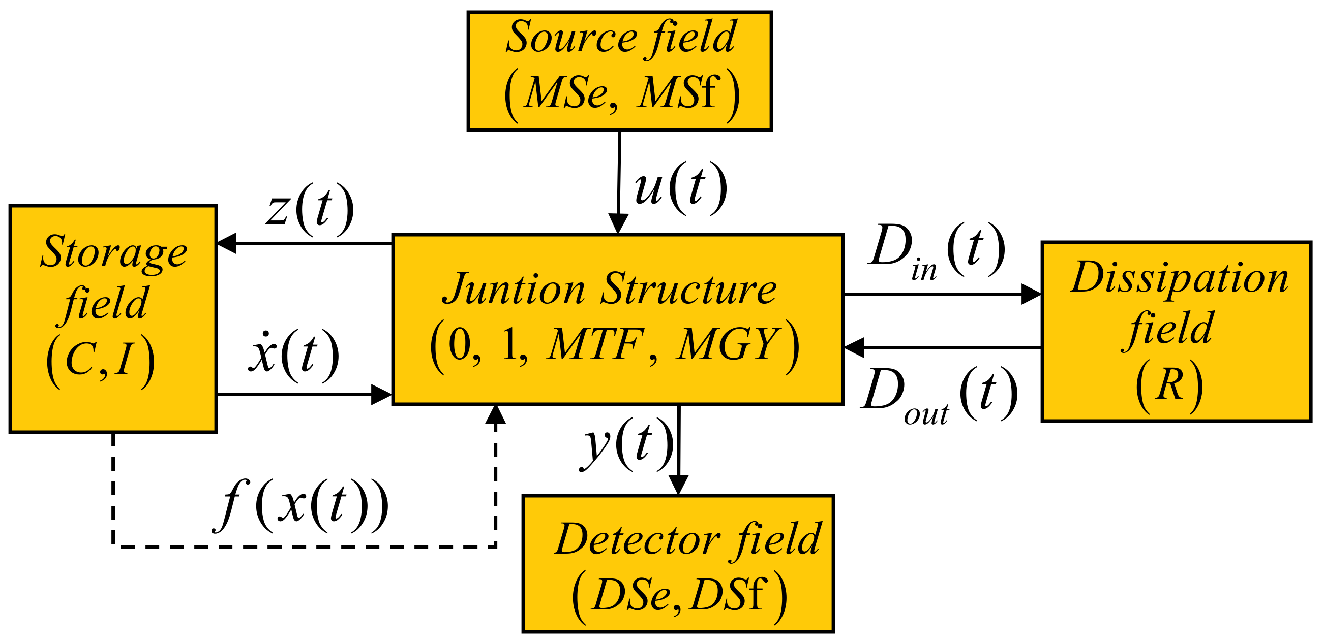
• The input $u\left(t\right)\in {\mathfrak{R}}^p$ obtained from a source field denoted by $\left(MSe,M{S}_f\right)$.
• The output $y\left(t\right)\in {\mathfrak{R}}^q$ obtained from a detector field denoted by $\left(DSe,D{S}_f\right)$.
• The state variables $x\left(t\right)\in {\mathfrak{R}}^n$ and the co-energy vector $z\left(t\right)\in {\mathfrak{R}}^n$ obtained from an energy storage field denoted by $\left(C,I\right)$ that defines the energy variables $q\left(t\right)$ and $p\left(t\right)$ associated with C and I elements.
• The variables $D_{in}\left(t\right)\in {\mathfrak{R}}^r$ and $D_{out}\left(t\right)\in {\mathfrak{R}}^r$ obtained from an energy dissipation field denoted by R, which are a mixture of the power variables $e\left(t\right)$ and $f\left(t\right)$ indicating the energy exchanges between the dissipation field and the junction structure.
• The class of the nonlinear systems obtained from the feedback between the storage field and the junction structure determines that $MTF$ and $MGY$ can be modulated by a state variables function $f\left(x\left(t\right)\right)$.

The junction structure for the class of nonlinear systems is defined by:

$$\left[\begin{array}{c}\stackrel{•}{x}\left(t\right)\\ D_{in}\left(t\right)\\ y\left(t\right)\end{array}\right]=\left[\begin{array}{ccc}{S}_{11}\left(x\right)& S_{12}\left(x\right)& S_{13}\left(x\right)\\ S_{21}\left(x\right)& S_{22}\left(x\right)& S_{23}\left(x\right)\\ S_{31}\left(x\right)& S_{32}\left(x\right)& S_{33}\left(x\right)\end{array}\right]\left[\begin{array}{c}z\left(t\right)\\ D_{out}\left(t\right)\\ u\left(t\right)\end{array}\right]$$

(17)

with the constitutive relationships for the storage and dissipation elements expressed by:

$$\begin{array}{ccc}\hfill z\left(t\right)& =& Fx\left(t\right)\hfill \end{array}$$

(18)

$$\begin{array}{ccc}\hfill D_{out}\left(t\right)& =& L{D}_{in}\left(t\right)\hfill \end{array}$$

(19)

From the second line of (17) with (19),

$$D_{in}\left(t\right)={\left[I-S_{22}\left(x\right)L\right]}^{-1}\left[S_{21}\left(x\right)z\left(t\right)+S_{23}\left(x\right)u\left(t\right)\right]$$

(20)

substituting (20) into the first line of (17) with (19),

$$\stackrel{•}{x}\left(t\right)=S_{11}\left(x\right)z\left(t\right)+S_{12}\left(x\right)L{\left[I-S_{22}\left(x\right)L\right]}^{-1}\left[S_{21}\left(x\right)z\left(t\right)+S_{23}\left(x\right)u\left(t\right)\right]+S_{13}\left(x\right)u\left(t\right)$$

the nonlinear state equation is given by:

$$\stackrel{•}{x}\left(t\right)=A\left(x\right)x\left(t\right)+B\left(x\right)u\left(t\right)$$

(21)

where the matrix relating the states and the inputs are:

$$\begin{array}{ccc}\hfill A\left(x\right)& =& \left[S_{11}\left(x\right)+S_{12}\left(x\right)M\left(x\right)S_{21}\left(x\right)\right]F\hfill \end{array}$$

(22)

$$\begin{array}{ccc}\hfill B\left(x\right)& =& S_{13}\left(x\right)+S_{12}\left(x\right)M\left(x\right)S_{23}\left(x\right)\hfill \end{array}$$

(23)

with nonlinear algebraic loops:

$$M\left(x\right)=L{\left[I-S_{22}\left(x\right)L\right]}^{-1}$$

(24)

From the third line of (17) with (20) and (19),

$$y\left(t\right)=S_{31}\left(x\right)z\left(t\right)+S_{32}\left(x\right)L{\left[I-S_{22}\left(x\right)L\right]}^{-1}\left[S_{21}\left(x\right)z\left(t\right)+S_{23}\left(x\right)u\left(t\right)\right]+S_{33}\left(x\right)u\left(t\right)$$

the nonlinear output equation is expressed by:

$$y\left(t\right)=C\left(x\right)x\left(t\right)+D\left(x\right)u\left(t\right)$$

(25)

where:

$$\begin{array}{ccc}\hfill C\left(x\right)& =& \left[S_{31}\left(x\right)+S_{32}\left(x\right)M\left(x\right)S_{21}\left(x\right)\right]F\hfill \end{array}$$

(26)

$$\begin{array}{ccc}\hfill D\left(x\right)& =& S_{33}\left(x\right)+S_{32}\left(x\right)M\left(x\right)S_{23}\left(x\right)\hfill \end{array}$$

(27)

The linearization of a class of nonlinear systems in a bond graph approach is presented in [27]. However, a junction structure of the linearized bond graph model for this paper is shown in Figure 2.

The scheme of the linearized bond graph model of Figure 2 describes:

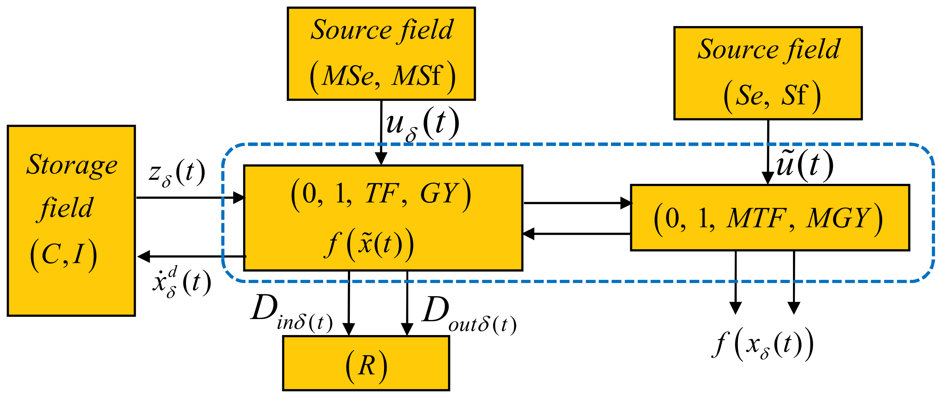
• The deviation of the state variables $x_{\delta }\left(t\right)$ with the corresponding co-energy vector $z_{\delta }\left(t\right)$.
• Changes or perturbations of the inputs $u_{\delta }\left(t\right)$ through modulated sources $\left(M{S}_e,M{S}_f\right)$.
• The deviation relationships between junction structure and dissipation elements given by $D_{in\delta }\left(t\right)$ and $D_{out\delta }\left(t\right)$.
• The junction structure is divided by the original junction structure with $\left(TF,GY\right)$ elements modulated by nominal trajectory $\tilde{x}\left(t\right)$ and a new junction structure with $\left(MTF,MGY\right)$ elements modulated by state variables $x_{\delta }\left(t\right)$ due to the linearization process in the physical domain.
• New $\left(S_e,S_f\right)$ sources with nominal trajectory values $\tilde{u}\left(t\right)$ due to new causal paths required in linearization.

At the end of this section, the new causal paths containing the new sources and the corresponding junction structure will be explained.

The linearized state equation with the corresponding output are described by:

$$\left[\begin{array}{c}{\stackrel{•}{x}}_{\delta }\left(t\right)\\ D_{in\delta }\left(t\right)\\ y_{\delta }\left(t\right)\end{array}\right]=\left[\begin{array}{cccc}{S}_{11}\left(\tilde{x}\right)& S_{12}\left(\tilde{x}\right)& S_{13}\left(\tilde{x}\right)& S_{14}\left(z_{\delta }\right)\\ S_{21}\left(\tilde{x}\right)& S_{22}\left(\tilde{x}\right)& S_{23}\left(\tilde{x}\right)& 0\\ S_{31}\left(\tilde{x}\right)& S_{32}\left(\tilde{x}\right)& S_{33}\left(\tilde{x}\right)& 0\end{array}\right]\left[\begin{array}{c}{z}_{\delta }\left(t\right)\\ D_{out\delta }\left(t\right)\\ u_{\delta }\left(t\right)\\ \tilde{u}\left(t\right)\end{array}\right]$$

(28)

with the constitutive relationships for the storage and dissipation elements described by:

$$\begin{array}{ccc}\hfill z_{\delta }\left(t\right)& =& F{x}_{\delta }\left(t\right)\hfill \end{array}$$

(29)

$$\begin{array}{ccc}\hfill D_{out\delta }\left(t\right)& =& L{D}_{in\delta }\left(t\right)\hfill \end{array}$$

(30)

From the second line of (28) with (30),

$$D_{in\delta }\left(t\right)={\left[I-S_{22}\left(\tilde{x}\right)L\right]}^{-1}\left[S_{21}\left(\tilde{x}\right)z_{\delta }\left(t\right)+S_{23}\left(\tilde{x}\right)u_{\delta }\left(t\right)\right]$$

(31)

and substituting (31) into the first line of (28),

$$\begin{array}{ccc}\hfill {\stackrel{•}{x}}_{\delta }\left(t\right)& =& S_{11}\left(\tilde{x}\right)z_{\delta }\left(t\right)+S_{12}\left(\tilde{x}\right)L{\left[I-S_{22}\left(\tilde{x}\right)L\right]}^{-1}\left[S_{21}\left(\tilde{x}\right)z_{\delta }\left(t\right)+S_{23}\left(\tilde{x}\right)u_{\delta }\left(t\right)\right]\hfill \\ & & +S_{13}\left(\tilde{x}\right)u_{\delta }\left(t\right)+S_{14}\left(z_{\delta }\right)\tilde{u}\left(t\right)\hfill \end{array}$$

(32)

with:

$$M\left(\tilde{x}\right)=L{\left[I-S_{22}\left(\tilde{x}\right)L\right]}^{-1}$$

(33)

then (32) can be written as:

$$\begin{array}{ccc}\hfill {\stackrel{•}{x}}_{\delta }\left(t\right)& =& \left[S_{11}\left(\tilde{x}\right)+S_{12}\left(\tilde{x}\right)M\left(\tilde{x}\right)S_{21}\left(\tilde{x}\right)\right]z_{\delta }\left(t\right)+S_{14}\left(z_{\delta }\right)\tilde{u}\left(t\right)\hfill \\ & & +\left[S_{13}\left(\tilde{x}\right)+S_{12}\left(\tilde{x}\right)M\left(\tilde{x}\right)S_{23}\left(\tilde{x}\right)\right]u_{\delta }\left(t\right)\hfill \end{array}$$

(34)

The term due to new causal paths for linearization is defined by:

$$S_{14}\left(z_{\delta }\right)\tilde{u}\left(t\right)=S_{14}\prime \left(\tilde{x}\right)x_{\delta }\left(t\right)$$

(35)

and the state equation for the linearized model is expressed by:

$${\stackrel{•}{x}}_{\delta }\left(t\right)=A_{\delta }{x}_{\delta }\left(t\right)+B_{\delta }{u}_{\delta }\left(t\right)$$

(36)

where the state and input matrices for the linearized system are described by:

$$\begin{array}{ccc}\hfill A_{\delta }& =& \left[S_{11}\left(\tilde{x}\right)+S_{12}\left(\tilde{x}\right)M\left(\tilde{x}\right)S_{21}\left(\tilde{x}\right)+S_{14}\prime \left(\tilde{x}\right)\right]F\hfill \end{array}$$

(37)

$$\begin{array}{ccc}\hfill B_{\delta }& =& S_{13}\left(\tilde{x}\right)+S_{12}\left(\tilde{x}\right)M\left(\tilde{x}\right)S_{23}\left(\tilde{x}\right)\hfill \end{array}$$

(38)

From the third line of (28) with (31), (30) and (33),

$$y_{\delta }\left(t\right)=S_{31}\left(\tilde{x}\right)z_{\delta }\left(t\right)+S_{23}\left(\tilde{x}\right)M\left(\tilde{x}\right)\left[S_{21}\left(\tilde{x}\right)z_{\delta }\left(t\right)+S_{23}\left(\tilde{x}\right)u_{\delta }\left(t\right)\right]+S_{33}\left(\tilde{x}\right)u_{\delta }\left(t\right)$$

then the output equation is defined by:

$$y_{\delta }\left(t\right)=C_{\delta }{x}_{\delta }\left(t\right)+D_{\delta }{u}_{\delta }\left(t\right)$$

(39)

where the matrices relating the states and the inputs are:

$$\begin{array}{ccc}\hfill C_{\delta }& =& \left[S_{31}\left(\tilde{x}\right)+S_{23}\left(\tilde{x}\right)M\left(\tilde{x}\right)S_{21}\left(\tilde{x}\right)\right]F\hfill \end{array}$$

(40)

$$\begin{array}{ccc}\hfill D_{\delta }& =& S_{33}\left(\tilde{x}\right)+S_{23}\left(\tilde{x}\right)M\left(\tilde{x}\right)S_{23}\left(\tilde{x}\right)\hfill \end{array}$$

(41)

The class of nonlinear systems applied in this paper are systems with products of state variables. The nonlinear bond graph models defined by (21) are linearized to obtain (36). Thus, the linearized bond graph models are constructed according to the steps described in the following Procedure 1:

Procedure 1.

• The linearization is in the vicinity of a known nominal trajectory $\left(\tilde{x},\tilde{u}\right)$.
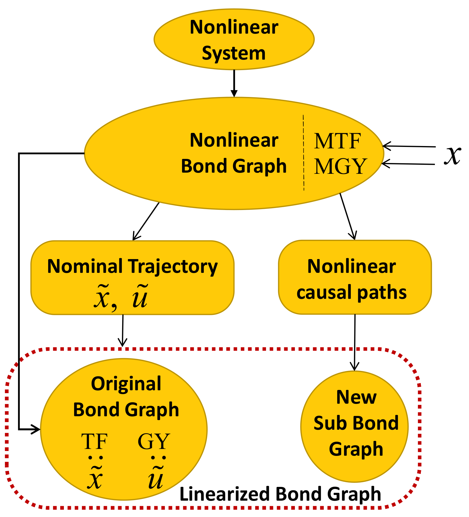
• The original nonlinear bond graph is with $MTF$ and/or $MGY$ where these two-port elements are changed by $TF$ and/or $GY$ modulated by $\left(\tilde{x},\tilde{u}\right)$, respectively.
• New causal paths are added. These nonlinear causal paths begin at the $\left(I_i,C_i\right)$ element, through one of $\left(MTF,MGY\right)$ modulated by a state variable, and arrive at $\left(I_j,C_j\right)$. The new causal paths are introduced by replacing $\left(I_i,C_i\right)$ and $\left(I_j,C_j\right)$ by $\left(MS{e}_i,MS{f}_i\right)$ evaluated at the nominal trajectory.

A diagram of the linearization described in Procedure 1 is shown in Figure 3.

This procedure is a reduced version of the methodology proposed in [27]. The concatenation of several linearized bond graph models to obtain approximated state variables due to the trajectory signal inputs is presented in the next section.

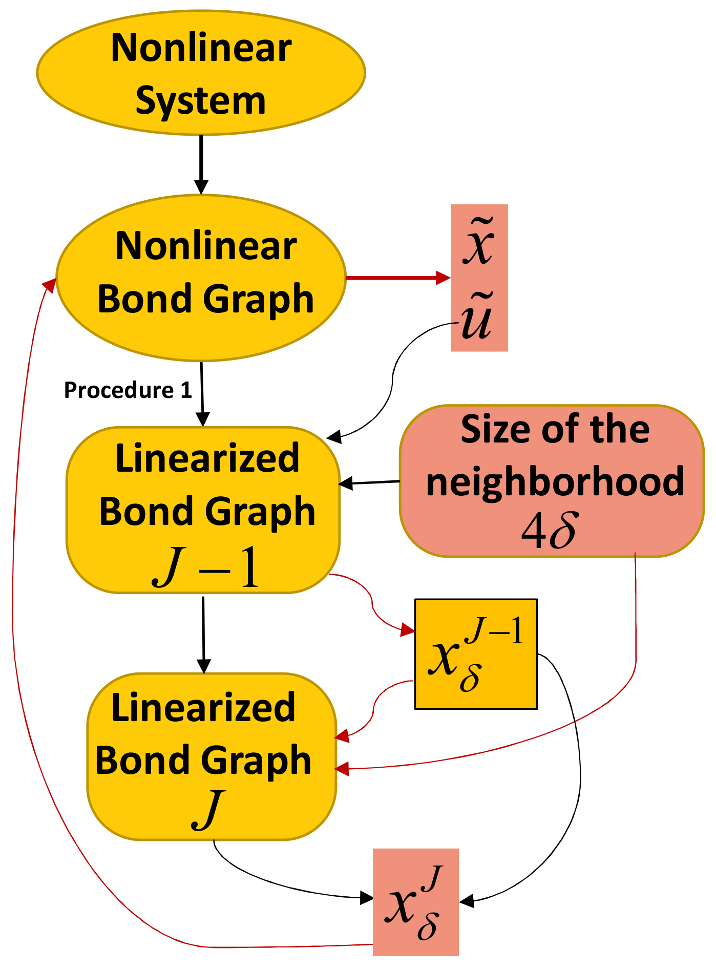
4. Approximation to Nonlinear Bond Graphs Based on Linearized Bond Graphs

Consider the linearization of a nonlinear bond graph (NBG) that determines a linearized bond graph (LBG). This LBG requires an initial state $x_0$ and the input $u_{\delta }\left(t\right)$ to determine the solution $x_{\delta }\left(t\right)$. In this paper, $u_{\delta }\left(t\right)$ is interpreted as the size of the neighborhood where the linearization can be applied.

Hence, the nonlinear system is linearized at an operation point and the size of the neighborhood is considered small and then continues to feed the state variables by changing the operating point to sweep the original signal, as shown in Figure 4.

According to Figure 4, the linearized bond graph $J-1$ determines the solution of the system from $t_0$ to $t_1$ being the condition to the linearized bond graph J to obtain the output at $t_2$. This connection is called in this paper dynamic linearization and can be used for many concatenated stages of linearization, which is formalized in the following lemma.

Lemma 1.

Consider a class of nonlinear systems modeled by bond graphs described by (21) whose linearization is expressed by (36) under a nominal operation point due to the linearized bond graph; then an approximated performance of the state variables connecting a recursive form of linearized bond graphs according to Figure 4 where $u_{\delta }\left(t\right)$ is the size of the neighborhood and the initial state is changed by the state variable solution is obtained.

Proof. 

The nonlinear system is defined by $\stackrel{•}{x}\left(t\right)=A\left(x\right)x\left(t\right)+B\left(x\right)u\left(t\right)$ with $x\left(t_0\right)=x_0$ whose nonlinear bond graph is shown in Figure 1. The linearization is defined by ${\stackrel{•}{x}}_{\delta }\left(t\right)=A_{\delta }{x}_{\delta }\left(t\right)+B_{\delta }{u}_{\delta }\left(t\right)$ under the nominal trajectory $\tilde{x}\left(t\right)$ whose linearized bond graph is shown in Figure 2 and then the exact solution is given by:

$$x\left(t\right)=x_{\delta }\left(t\right)+x_0+O\left(\epsilon \right)$$

□

Proof. 

Consider a trajectory from $t_0$ to $t_2$ through $t_1$ where $t_0\prec t_1\prec t_2$. The exact solution at $t_1$ is:

$$x\left(t_1\right)=x_{\delta }\left(t_1\right)+x_0\left(t_0\right)+O\left(\epsilon \right)$$

where:

$$x_{\delta }\left(t_1\right)={\int }_{t_0}^{t_1}{\stackrel{•}{x}}_{\delta }\left(t\right)dt$$

then:

$$x\left(t_1\right)={\int }_{t_0}^{t_1}{\stackrel{•}{x}}_{\delta }\left(t\right)dt+x_0\left(t_0\right)+O\left(\epsilon \right)$$

For $t_2$, the exact solution is given by:

$$x\left(t_2\right)=x_{\delta }\left(t_2\right)+x_0\left(t_1\right)+O\left(\epsilon \right)$$

where:

$$x\left(t_2\right)={\int }_{t_1}^{t_2}{\stackrel{•}{x}}_{\delta }\left(t\right)dt+x_0\left(t_1\right)+O\left(\epsilon \right)$$

using from $t_0$ to $t_2$

$$x\left(t_2\right)={\int }_{t_0}^{t_2}{\stackrel{•}{x}}_{\delta }\left(t\right)dt+x_0\left(t_0\right)+O\left(\epsilon \right)$$

then:

$$x\left(t_2\right)={\int }_{t_0}^{t_1}{\stackrel{•}{x}}_{\delta }\left(t\right)dt+{\int }_{t_1}^{t_2}{\stackrel{•}{x}}_{\delta }\left(t\right)dt+x_0\left(t_0\right)+O\left(\epsilon \right)$$

for any time:

$$x\left(t_n\right)={\int }_{t_0}^{t_1}{\stackrel{•}{x}}_{\delta }\left(t\right)dt+{\int }_{t_1}^{t_2}{\stackrel{•}{x}}_{\delta }\left(t\right)dt+\cdots +{\int }_{t_{n-1}}^{t_n}{\stackrel{•}{x}}_{\delta }\left(t\right)dt+x_0\left(t_0\right)+O\left(\epsilon \right)$$

(42)

thus, for each term of (42), i.e., the integral ${\int }_{t_0}^{t_1}{\stackrel{•}{x}}_{\delta }\left(t\right)dt$ can be obtained by a linearized bond graph from $t_0$ to $t_1$ with $x_0$ and the solution of this model is used to introduce the next linearized bond graph model that solves ${\int }_{t_1}^{t_2}{\stackrel{•}{x}}_{\delta }\left(t\right)dt$ from $t_1$ to $t_2$ with $x_1$ and so on; then the approximated state variables for $x\left(t_n\right)$ can be obtained by connecting linearized bond graph models with the necessary conditions defined by Lemma 1, which is proven. □

In order to apply the proposed Lemma 1 for the approximation of nonlinear systems using linearized bond graph models, the following procedure describes the necessary steps needed to achieve this objective.

Procedure 2.

• Obtain the nonlinear bond graph corresponding to the nonlinear system.
• Analyze the behavior of the nonlinear model and find an operating point that will be the first point where the system will start to be linearized.
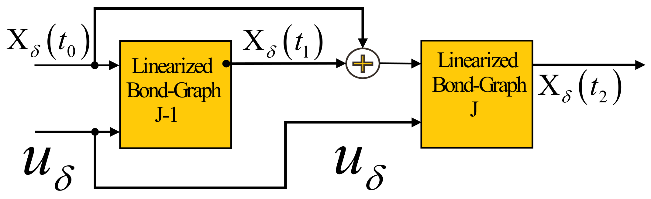
• Determine the increase of the inputs that will be used to determine for subsequent operating points of the linearized system.
• Obtain the linearized bond graph model.
• The new output is the sum of the operating point values found in step 2 and the increment produced at the moment.
• Additional sources due to a linearized bond graph will be fed by the outputs found in step 5.
• The value of the increment in the state variables will be updated to recalculate the next operating point values.

The process of dynamic linearization given in Procedure 2 is illustrated in Figure 5.

A nonlinear electromechanical system is used in the next section to apply the proposed methodology.

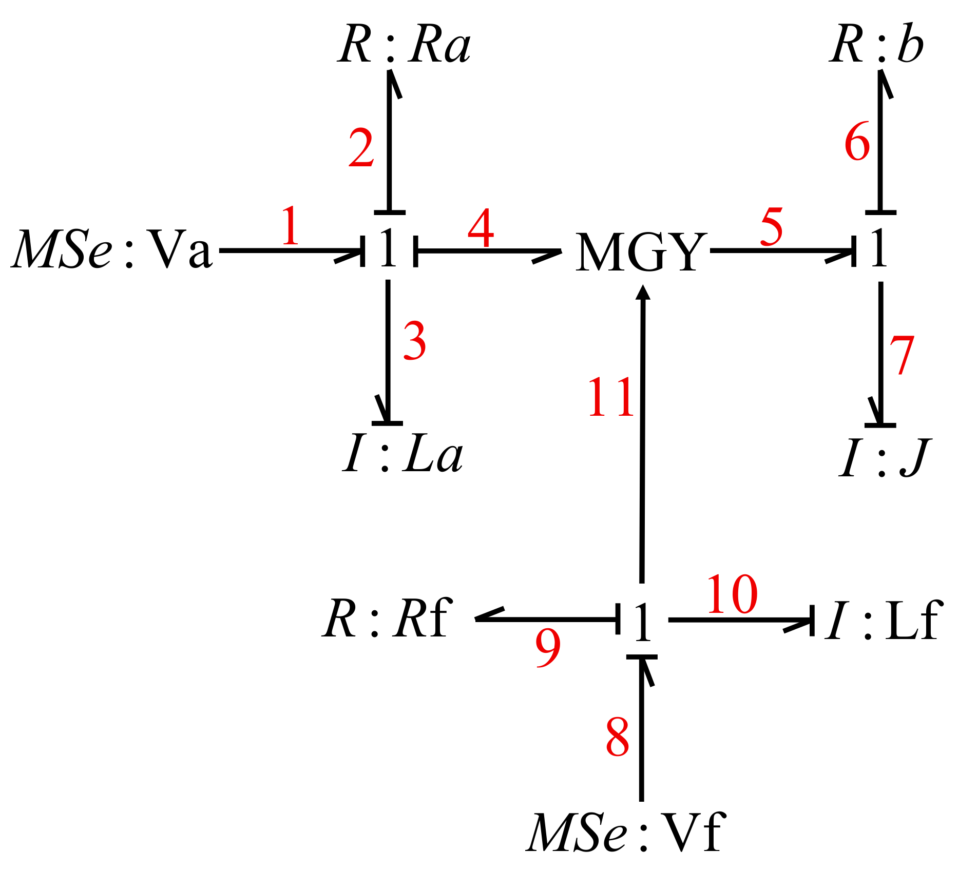
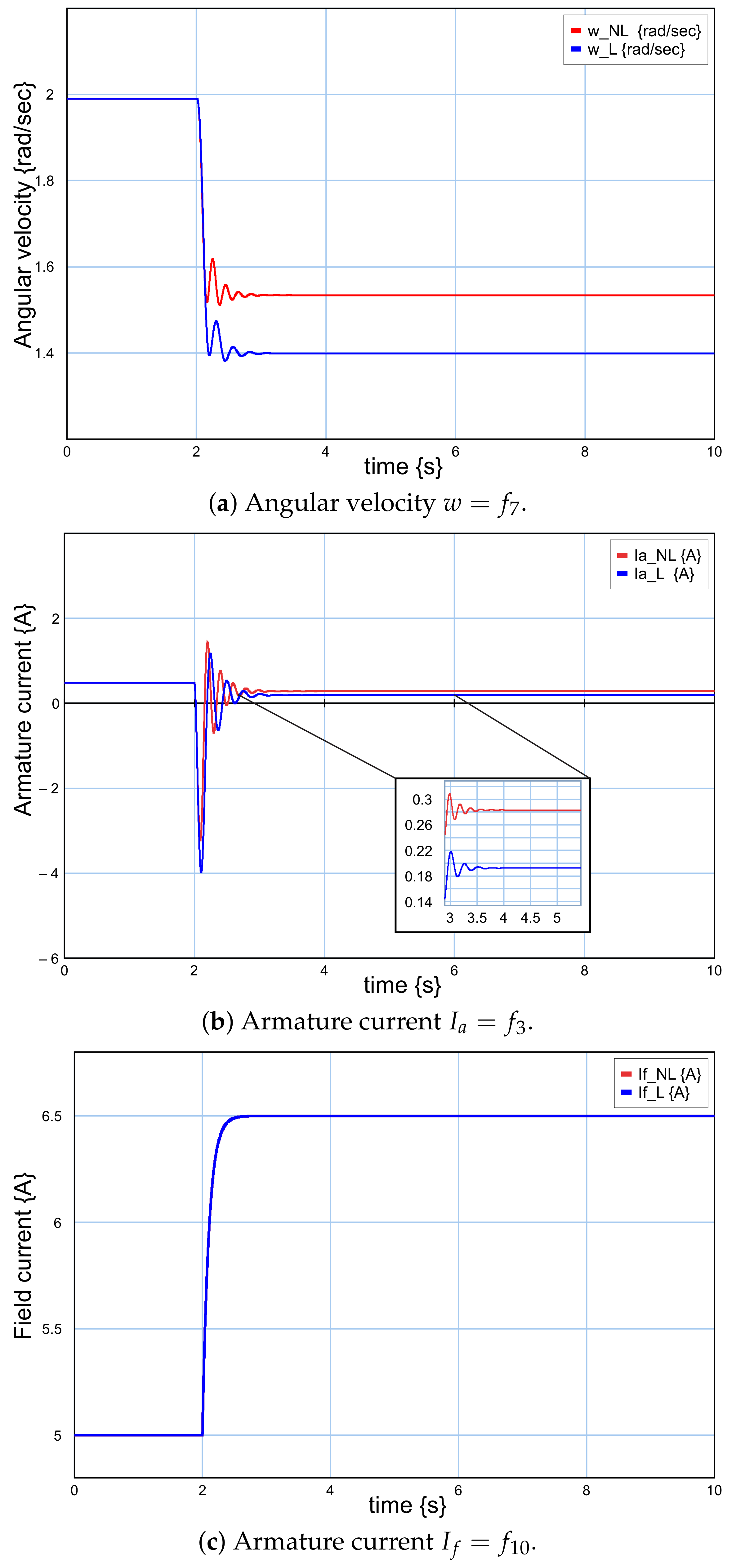
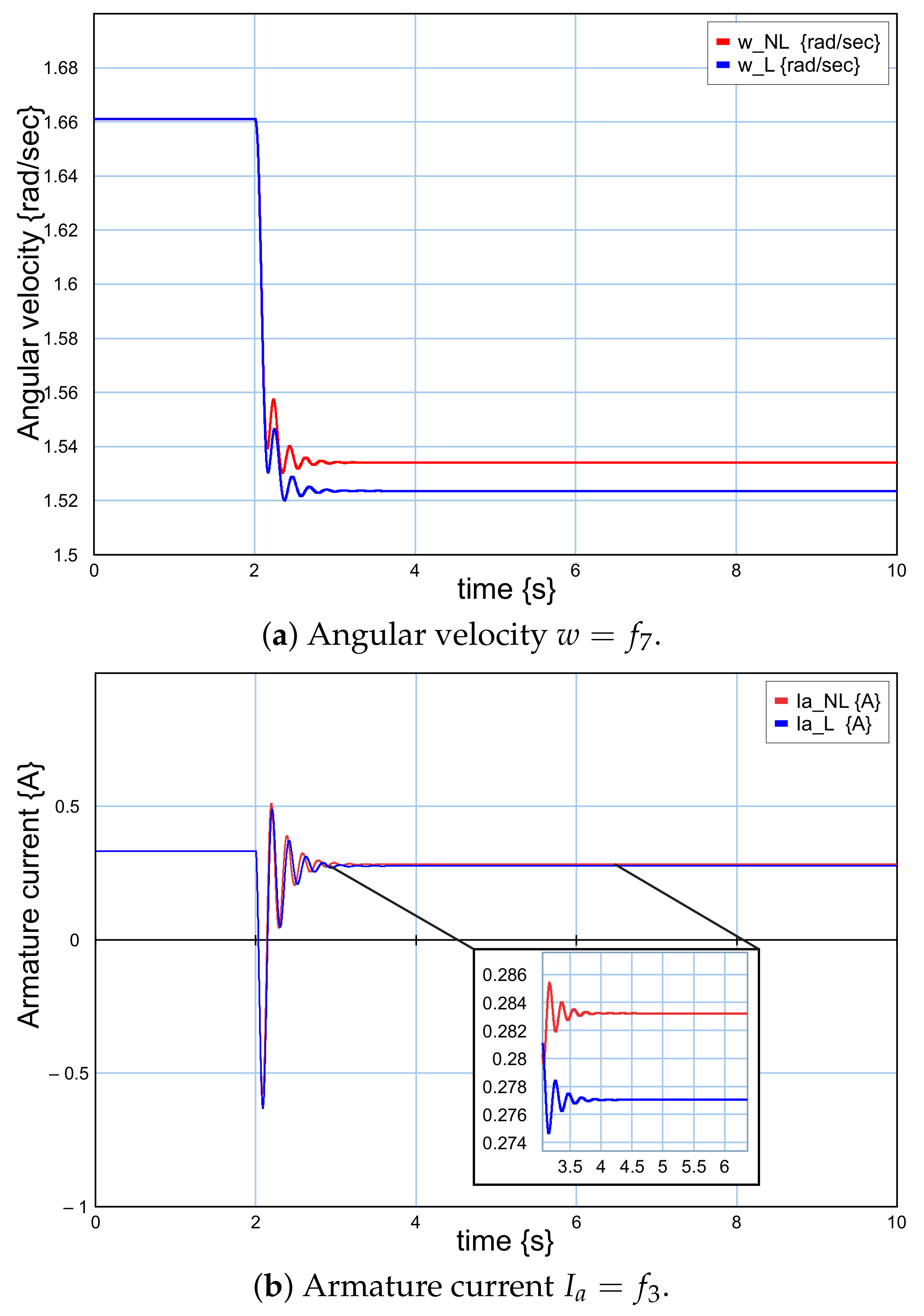
5. Case Study

A nonlinear DC motor schematic model is shown in Figure 6. This system is a electromechanical model formed by the armature winding with resistance, inductance and voltage, namely $R_a$, $L_a$ and $V_a$, respectively; and the field winding with resistance, inductance and voltage, $R_f,$ $L_f$ and $V_f$, respectively; the inertia moment J and friction coefficient b represent the mechanical part of the system.

The use of linearized bond graphs to obtain an approximate response to the nonlinear system applying Procedure 2 is developed as follows. The nonlinear bond graph of the DC motor is illustrated in Figure 7.

This NBG contains three parts:

-

The armature winding formed by the connection of $R:R_a,$ $I:L_a$ and $MSe:V_a$ to a junction 1 indicating that the armature current $\left(I_a\right)$ is the same in these elements.

-

The field winding formed by the connection of $R:R_f,$ $I:L_f$ and $MSe:V_f$ to a junction 1 indicating that the field current $\left(I_f\right)$ is the same in these elements.

-

The mechanical component by the connection of $R:b$ and $I:J$ to a junction 1 indicating that the angular velocity $\left(w\right)$ is the same in these elements.

-

The electrical energy conversion to mechanical energy is realized with an $MGY$ element modulated by an active bond due to the field current.

The key vectors of the NBG are described by:

$$x=\left[\begin{array}{c}{p}_3\\ p_7\\ p_{10}\end{array}\right];\stackrel{•}{x}=\left[\begin{array}{c}{e}_3\\ e_7\\ e_{10}\end{array}\right];z=\left[\begin{array}{c}{f}_3\\ f_7\\ f_{10}\end{array}\right];D_{in}=\left[\begin{array}{c}{f}_2\\ f_6\\ f_9\end{array}\right];D_{out}=\left[\begin{array}{c}{e}_2\\ e_6\\ e_9\end{array}\right];u=\left[\begin{array}{c}{e}_1\\ e_8\end{array}\right]$$

with the constitutive relationships:

$$\begin{array}{ccc}\hfill F& =& diag\left\{\frac{1}{L_a},\frac{1}{J},\frac{1}{L_f}\right\}\hfill \end{array}$$

(43)

$$\begin{array}{ccc}\hfill L& =& diag\left\{R_a,b,R_f\right\}\hfill \end{array}$$

(44)

and the nonlinear junction structure is given by:

$$\left[\begin{array}{c}{e}_3\\ e_7\\ e_{10}\\ f_2\\ f_6\\ f_9\end{array}\right]=\left[\begin{array}{cccccccc}0& -f_{10}& 0& -1& 0& 0& 1& 0\\ f_{10}& 0& 0& 0& -1& 0& 0& 0\\ 0& 0& 0& 0& 0& -1& 0& 1\\ 0& 0& 0& 0& 0& 0& 0& 0\\ 0& 0& 0& 0& 0& 0& 0& 0\\ 0& 0& 0& 0& 0& 0& 0& 0\end{array}\right]\left[\begin{array}{c}{f}_3\\ f_7\\ f_{10}\\ e_2\\ e_6\\ e_9\\ e_1\\ e_8\end{array}\right]$$

(45)

In this case, only the submatrix $S_{11}\left(x\right)$ depends on a state variable and the rest of the submatrices of the junction structure are constants. Additionally, $S_{22}\left(x\right)=0$ and thus $M\left(x\right)=L$.

From (22), (43), (44) and (45), the state matrix for the linearized system is described by:

$$A\left(x\right)=\left[\begin{array}{ccc}\frac{-R_a}{L_a}& \frac{-f_{10}}{J}& 0\\ \frac{f_{10}}{L_a}& \frac{-b}{J}& 0\\ 0& 0& \frac{-R_f}{L_f}\end{array}\right]$$

(46)

and from (23), (44) and (45), the input matrix for this linearized system is:

$$B\left(x\right)=\left[\begin{array}{cc}1& 0\\ 0& 0\\ 0& 1\end{array}\right]$$

(47)

By substituting (46) and (47) into (21), the nonlinear system is described by:

$$\begin{array}{ccc}\hfill {\stackrel{•}{x}}_1& =& \frac{-R_a}{L_a}{x}_1-\frac{x_2{x}_3}{J{L}_f}+u_1\hfill \end{array}$$

(48)

$$\begin{array}{ccc}\hfill {\stackrel{•}{x}}_2& =& \frac{x_1{x}_3}{L_a{L}_f}-\frac{b}{J}{x}_2\hfill \end{array}$$

(49)

$$\begin{array}{ccc}\hfill {\stackrel{•}{x}}_3& =& \frac{-R_f}{L_f}{x}_3+u_2\hfill \end{array}$$

(50)

In order to apply the linearization procedure (Procedure 1) in a bond graph approach, the initial point is $x_o={\left[\begin{array}{ccc}{x}_{o1}& x_{o2}& x_{o3}\end{array}\right]}^T$ and the nonlinear causal paths are given by:

• From $I:L_a$ to $I:J$ is $3-4-5-7$;
• From $I:J$ to $I:L_a$ is $7-5-4-3$.

Once nonlinear causal paths are identified, the additional bonds used to consider these terms on the linearization process are shown in Figure 8.

By joining the initial bond graph and additional bonds, the linearized bond graph is illustrated in Figure 9.

The key vectors of the LBG are:

$$\begin{array}{ccc}\hfill x_{\delta }& =& \left[\begin{array}{c}{p}_3\\ p_7\\ p_{10}\end{array}\right];{\stackrel{•}{x}}_{\delta }=\left[\begin{array}{c}{e}_3\\ e_7\\ e_{10}\end{array}\right];z_{\delta }=\left[\begin{array}{c}{f}_3\\ f_7\\ f_{10}\end{array}\right];D_{in\delta }=\left[\begin{array}{c}{f}_2\\ f_6\\ f_9\end{array}\right];D_{in\delta }=\left[\begin{array}{c}{f}_2\\ f_6\\ f_9\end{array}\right]\hfill \\ \hfill u_{\delta }& =& \left[\begin{array}{c}{e}_1\\ e_8\end{array}\right];\tilde{u}=\left[\begin{array}{c}{f}_{12}\\ f_{15}\end{array}\right]=\left[\begin{array}{c}\widetilde{I_a}\\ \tilde{w}\end{array}\right]\hfill \end{array}$$

with the linearized junction structure given by:

$$\left[\begin{array}{c}{e}_3\\ e_7\\ e_{10}\\ f_2\\ f_6\\ f_9\end{array}\right]=\left[\begin{array}{cccccccccc}0& -\widetilde{I_f}& 0& -1& 0& 0& 1& 0& 0& -f_{10}\\ \widetilde{I_f}& 0& 0& 0& -1& 0& 0& 0& f_{10}& 0\\ 0& 0& 0& 0& 0& -1& 0& 1& 0& 0\\ 1& 0& 0& 0& 0& 0& 0& 0& 0& 0\\ 0& 1& 0& 0& 0& 0& 0& 0& 0& 0\\ 0& 0& 1& 0& 0& 0& 0& 0& 0& 0\end{array}\right]\left[\begin{array}{c}{f}_3\\ f_7\\ f_{10}\\ e_2\\ e_6\\ e_9\\ e_1\\ e_8\\ f_{12}\\ f_{15}\end{array}\right]$$

(51)

From (35) and (51),

$$S_{14}\prime \left(\tilde{x}\right)=\left[\begin{array}{ccc}0& 0& -\tilde{w}\\ 0& 0& \widetilde{I_a}\\ 0& 0& 0\end{array}\right]$$

(52)

From (37), (51) and (52) with (43),

$$A_{\delta }=\left[\begin{array}{ccc}\frac{-R_a}{L_a}& \frac{-\widetilde{I_f}}{J}& \frac{-\tilde{w}}{L_F}\\ \frac{\widetilde{I_f}}{L_a}& \frac{-b}{J}& \frac{-\widetilde{I_a}}{L_f}\\ 0& 0& \frac{-R_f}{L_f}\end{array}\right]$$

(53)

from (38) and (51),

$$B_{\delta }=\left[\begin{array}{cc}1& 0\\ 0& 0\\ 0& 1\end{array}\right]$$

(54)

and the linearized state equation is expressed by:

$${\stackrel{•}{x}}_{\delta }=\left[\begin{array}{ccc}\frac{-R_a}{L_a}& \frac{-\widetilde{I_f}}{J}& \frac{-\tilde{w}}{L_F}\\ \frac{\widetilde{I_f}}{L_a}& \frac{-b}{J}& \frac{-\widetilde{I_a}}{L_f}\\ 0& 0& \frac{-R_f}{L_f}\end{array}\right]x_{\delta }+\left[\begin{array}{cc}1& 0\\ 0& 0\\ 0& 1\end{array}\right]u_{\delta }$$

(55)

The numerical parameters of the nonlinear bond graph are listed in

Table 1. Parameters of the DC motor.

$R_a=0.1$ $\Omega$	$L_a=0.1$ H	$R_f=1$ $\Omega$	$L_f=1$ H
$b=1.2$ N-s/m	$J=4$ N-m-s${}^2$	$V_a=10$ V	$V_f=5$ V

.

The initial value for the state variables in the linearized bond graph model is:

$$\left[\begin{array}{c}\tilde{w}\\ \widetilde{I_a}\\ \widetilde{I_f}\end{array}\right]=\left[\begin{array}{c}7.961783439490366rad/s\\ 0.004777070063693411A\\ 0.5000000000000056A\end{array}\right]$$

(56)

The dynamic performances of this case study using different magnitudes for the neighborhoods are shown in Figure 10, Figure 11 and Figure 12. All of these figures show the state variables of the nonlinear bond graph of Figure 7 and of the linearized bond graph of Figure 9.

Figure 10 illustrates the responses with a single linearized model with the field winding voltage changed from $V_f=5$ V to $V_f=6.5$ V and when the neighborhood is $1.5$ V. In this case, we have a single linearization stage with a neighborhood of the size of the voltage change $V_f$. We do not have a good approximation of the angular velocity and the armature current of the nonlinear and linearized models. The field current is the same in the nonlinear and linearized models.

Now, the field winding voltage changes from $V_f=5$ V to $V_f=6.5$ V; however, the neighborhood size is $0.5$ V and thus it takes three steps of linearized models to reach the full $1.5$ V change, which is shown in Figure 11. Dynamic linearization has been applied by approximating the response of the linearized model to the nonlinear model.

Finally, we have the same change from $V_f=5$ V to $V_f=6.5$ V with neighborhood sizes of $0.1$ V requiring the use of 15 steps of linearized models, as shown in Figure 12. A better approximation of the linearized model has been achieved with small neighborhoods of $0.1$ V.

Undoubtedly, the use of smaller neighborhoods in the linearized bond graph models allows to obtain more exact results. Even though the number of recursive steps of the linearized model will be greater for current computer systems, this is not a big problem.

Bond graph methodology has been used as a graphical way of modeling systems. Additionally, analysis results of these systems have been obtained. Therefore, connecting linearized models in bond graphs and the traditional algebraic approach can be another way of providing other scopes to bond graphs.

6. Conclusions

The complexity of analysis of nonlinear systems opens up the possibility of alternate methods of using the widely used methodologies of linear systems. Hence, the solution of a class of nonlinear systems modeled in bond graphs using linearized bond graph models has been presented. To improve the approximation of the response of the linearized models, the application of dynamic linearization has been proposed. This is a type of recursive linearization that allows to have smaller neighborhoods to reduce errors between linearized models to nonlinear models. Thus, there is a symmetry between linearized models and nonlinear models in bond graphs A case study of a DC motor has been used to show the effectiveness of the methodology proposed in bond graphs. The simulation results showed that by decreasing the size of the neighborhood, a very good approximation of the solution of the nonlinear system was achieved. These results of the design of control strategies for nonlinear systems using linearized models in the physical domain can be extended.

References

- Verrelli, C.; Tomei, P.; Lorenzani, E.; Migliazza, G.; Immovilli, F. Nonlinear tracking control for sensorless permanent magnet synchronous motors with uncertainties. Control. Eng. Pract. 2017, 60, 157–170. [Google Scholar] [CrossRef]
- Asada, H.H.; Wu, F.; Girard, A.; Mayalu, M. A data-driven approach to precise linearization of nonlinear dynamical systems in augmented latent space. In Proceedings of the 2016 American Control Conference (ACC), Boston, MA, USA, 6–8 July 2016; pp. 1838–1844. [Google Scholar]
- Aguilar, O.; Tapia, R.; Rivas, I.; Minor, H. Adaptive Speed Controller for a Permanent Magnet Synchronous Motor. Nat. Eng. 2019, 11, 142–170. [Google Scholar] [CrossRef]
- Igarashi, Y.; Yamakita, M.; Ng, J.; Asada, H.H. MPC Performances for Nonlinear Systems Using Several Linearization Models. In Proceedings of the 2020 American Control Conference (ACC), Denver, CO, USA, 1–3 July 2020; pp. 2426–2431. [Google Scholar] [CrossRef]
- Khalil, H.K.; Grizzle, J.M. Nonlinear Systems; Prentice-Hall: Hoboken, NJ, USA, 2002; Volume 3. [Google Scholar]
- Khalil, H.K. Nonlinear Control, Global ed.; Pearson Education Limited: London, UK, 2015. [Google Scholar]
- Karnopp, D. Power and Energy in Linearized Physical Systems. J. Frankl. Inst. 1977, 303, 85–98. [Google Scholar] [CrossRef]
- Masoudi, R.; NcPhee, J. Application of Karhunen-Loeve decomposition and piecewise linearization to a physics-based battery model. Electrochem. Acta 2021, 365, 137093. [Google Scholar] [CrossRef]
- Anderson, P.M.; Fouad, A.A. Power System Control and Stability; Science Press: Beijing, China, 1986. [Google Scholar]
- Kundur, P. Power System Stability and Control; McGraw-Hill: New York, NY, USA, 1994. [Google Scholar]
- Grigsby, L.L. Power Systems Stability and Control, 3rd ed.; CRC Press: Boca Raton, FL, USA, 2012. [Google Scholar]
- Vittal, V.; McCalley, J.D.; Anderson, P.M.; Fouad, A.A. Power System Control and Stability, 3rd ed.; Wiley-IEEE Press: Hoboken, NJ, USA, 2019. [Google Scholar]
- Yang, D.C.H.; Tzeng, S.W. Simplification and Linearization of manipulator dynamics by the design of inertia distribution. Int. J. Robot. Res. 1986, 5, 120–128. [Google Scholar] [CrossRef]
- Orhanli, T.; Yilmaz, A. Analysis of Gait Dynamics with the Double Pendulum Model. In Proceedings of the 2019 27th Signal Processing and Communications Applications Conference (SIU), Sivas, Turkey, 24–26 April 2019; pp. 1–4. [Google Scholar] [CrossRef]
- Malgalhaes, F.C.; Hirokazu, W.E.; Correa, M.L.F. A linearized small-signal Thevenin-equivalent model of a voltage-controlled modular multilevel converter. Electr. Power Syst. Res. 2020, 182, 106231. [Google Scholar]
- Beauchamp, D.; Chugg, K.M. Linearization for High-Speed Current-Steering DACs Using Neural Networks. arXiv 2021, arXiv:2011.10642. [Google Scholar]
- Hernandez, M.; Messina, A.R. Recursive Linearization of Higher-Order for Power System Models. IEEE Trans. Power Syst. 2021, 36, 1206–1216. [Google Scholar] [CrossRef]
- Breedveld, P.C. Modeling and Simulation of Dynamic Systems Using Bond Graphs; EOLSS Publishers: Oxford, UK, 2008. [Google Scholar]
- Kypuros, J.A. System Dynamics and Control with Bond Graph Modeling; CRC Press: Boca Raton, FL, USA, 2013. [Google Scholar]
- Tenreiro, M.J.A.; Cunha, V.M.R. An Introduction to Bond Graph Modeling with Applications; CRC Press: Boca Raton, FL, USA, 2021. [Google Scholar]
- Karnopp, D.C.; Rosenberg, R. Systems Dynamics: A Unified Approach; Wiley John & Sons: Hoboken, NJ, USA, 2000. [Google Scholar]
- Sueur, C.; Dauphin-Tanguy, G. Bond graph approach for structural analysis of MIMO linear systems. J. Franklin Inst. 1991, 1, 55–70. [Google Scholar] [CrossRef]
- Borutzky, W. Bond Graph Methodology: Development and Analysis of Multidisciplinary Dynamic Systems Models; Springer: Berlin/Heidelberg, Germany, 2010. [Google Scholar]
- Borutzky, W. Bond Graph Modelling of Engineering Systems: Theory, Applications and Software Support; Springer: Berlin/Heidelberg, Germany, 2011. [Google Scholar]
- Zanj, A.; He, F.; Breedveld, P.C. An energy-based viscoelastic model for multiphysical systems: A Bond graph approach. In Proceedings of the 2016 IEEE International Conference on Systems, Man and Cybernetics (SMC), Budapest, Hungary, 9–12 October 2016; pp. 2214–2219. [Google Scholar] [CrossRef]
- Zanj, A.; He, F. Multiple-field systems dynamic modeling, Part I: Physical decomposition of multi-physical systems, a bond graph approach. In Proceedings of the 2017 8th International Conference on Mechanical and Aerospace Engineering (ICMAE), Prague, Czech Republic, 22–25 July 2017; pp. 661–666. [Google Scholar] [CrossRef]
- Gonzalez, G.; Galindo, R. A procedure to linearize a class of non-linear systems modelled by bond graphs. Math. Comput. Model. Dyn. Syst. 2015, 21, 38–57. [Google Scholar] [CrossRef]
- Sia, K.; Namaane, A.; M’Sirdi, N.K. A new structural approach for ARRs generation from linear & linearized bond graphs. In Proceedings of the 2011 International Conference on Communications, Computing and Control Applications (CCCA), Hammamet, Tunisia, 3–5 March 2011; pp. 1–6. [Google Scholar] [CrossRef]
- Al-Mashhadani, I.; Hadjiloucas, S. Linearized Bond Graph of Hodgkin-Huxley Memristor Neuron Model, CNNA 2016. In Proceedings of the 15th International Workshop on Cellular Nanoscale Networks and their Applications, Dresden, Germany, 23–25 August 2016; pp. 1–2. [Google Scholar]
- Gonzalez, G.; Ayala, G.; Barrera, N.; Padilla, J.A. Linearization of a class of non-linear systems modelled by multibond graphs. Math. Comput. Model. Dyn. Syst. 2019. [Google Scholar] [CrossRef]
- Rough, W.J. Linear System Theory; Prentice-Hall: Hoboken, NJ, USA, 1996. [Google Scholar]
- Kailath, T. Linear Systems; Prentice-Hall: Hoboken, NJ, USA, 1979. [Google Scholar]
- Chen, C.T. Linear System, Theory and Design, 3rd ed.; Holt, Rinehart and Winston: New York, NY, USA, 1998. [Google Scholar]
- Antsaklis, P.J.; Michel, A.N. Linear Systems; Springer Science & Business Media: Berlin/Heidelberg, Germany, 2006. [Google Scholar]