
An Unsupervised Learning Method for Attributed Network Based on Non-Euclidean Geometry


Abstract
:1. Introduction
2. Related Work
2.1. Hyperbolic Geometry
- Hyperboloid model. We first define the Minkowski space and the Minkowski product. The (n+1)-dimensional Minkowski space is a vector space endowed with the Minkowski inner product of the following form:
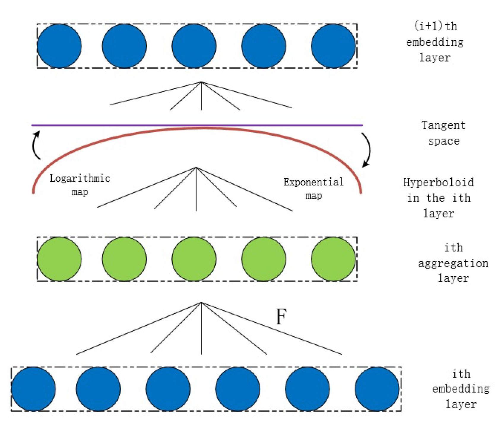
- Logarithmic and exponential maps.The hyperbolic space is a metric space, but not a vector space, and the tangent spaces are the local Euclidean spaces glued to the hyperbolic space. Therefore, in order to operate on vectors in the hyperbolic space, we must first map the corresponding points in the hyperbolic space to their tangent spaces, perform operations related to vectors in the Euclidean tangent spaces, and then map the resulting vector back to the hyperbolic space. It is worth noting that an exponential map can map points in a hyperbolic space to the corresponding tangent space, while a logarithmic map can map points in a tangent space back to the hyperbolic space, and in the hyperboloid model, both have simple closed forms.
- Parrallel Transport. If p and q are two points on the hyperboloid , then the parallel transport of the vector u from the tangent space at p to the tangent space at q is defined as
- Projections. The projection operation here is to project the vector onto the hyperboloid manifold and the corresponding tangent space, which is useful for the optimization process. Let ; then, it can be projected on the hyperboloid space in the following way:
- Hyperboloid linear transform. The usual linear transformation in the Euclidean space is multiplying the weight matrix by the embedding vector, and then adding the bias vector. However, the hyperbolic space itself is not a vector space, in which matrix multiplication cannot be carried out directly. As a consequence, we must map the points in the hyperbolic space to the tangent space at the origin by the logarithmic map, multiply by the weight matrix in the tangent space, and then pull the result back to the hyperbolic manifold by the exponential map, i.e.,
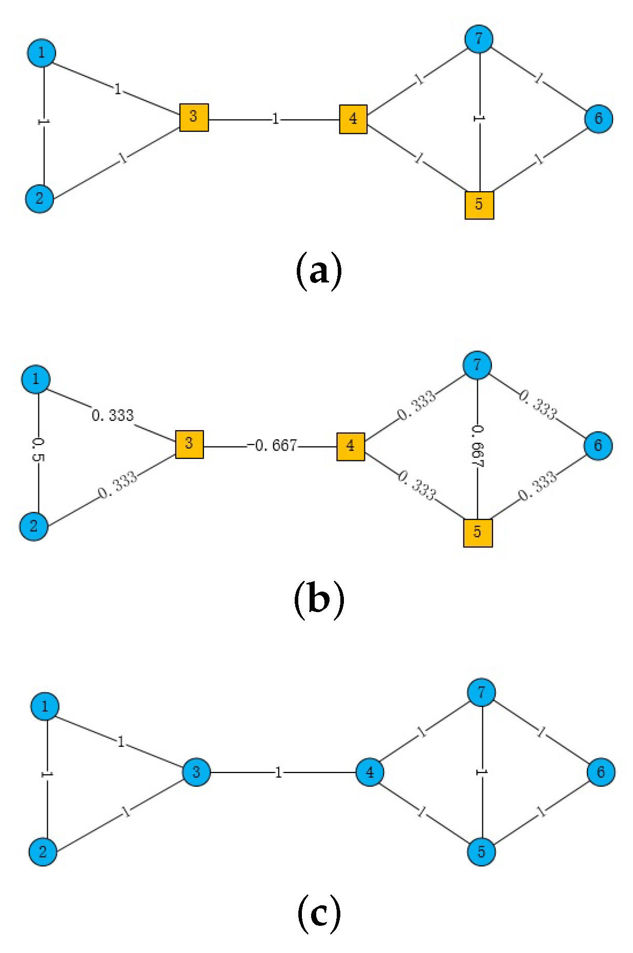
2.2. Ricci Curvature and Scalar Curvature
2.3. Related Work
3. Methods
3.1. Problem Setting
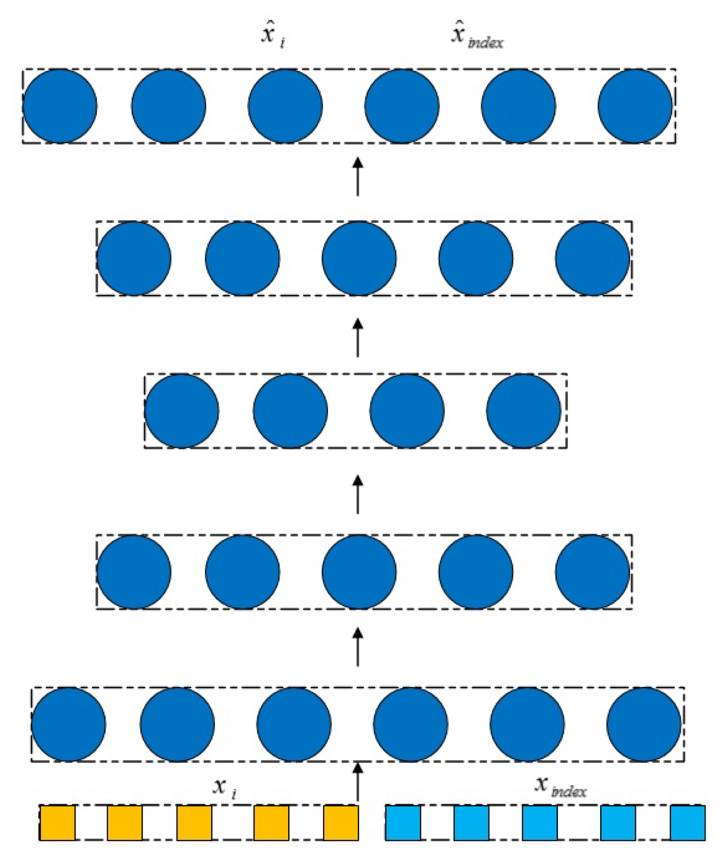
3.2. Non-Euclidean Autoencoder
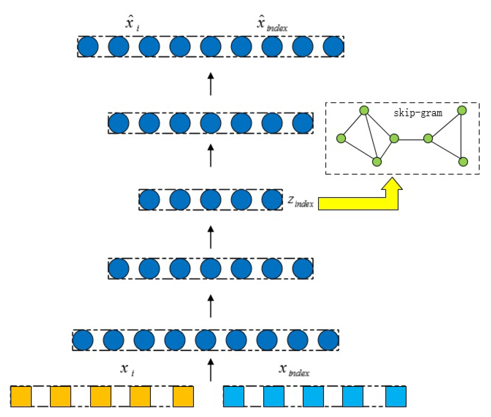
3.3. Skip-Gram Model Based on Ricci Curvature
3.4. RHAE Architecture
4. Experiment
4.1. Datasets
4.2. Baseline Methods Setup
4.3. Node Classification
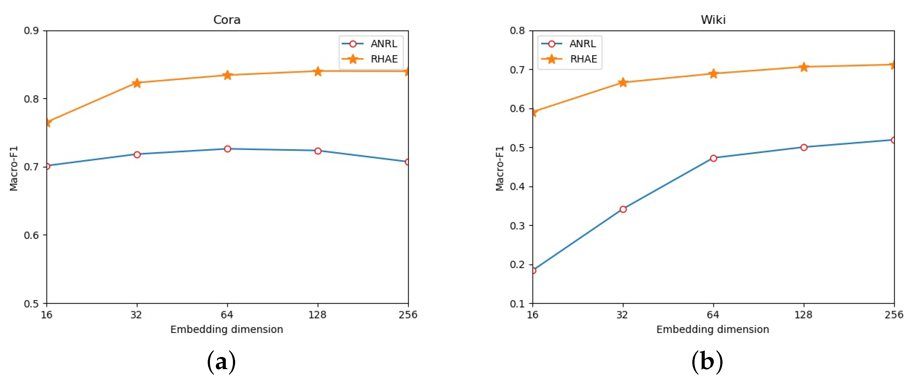
4.4. The Effect of Embedding Dimension
4.5. Training Time Comparison
5. Conclusions and Future Work
Author Contributions
Funding
Institutional Review Board Statement
Informed Consent Statement
Data Availability Statement
Conflicts of Interest
References
- Perozzi, B.; Al-Rfou, R.; Skiena, S. Deepwalk: Online learning of social representations. In Proceedings of the 20th ACM SIGKDD International Conference on Knowledge Discovery and Data Mining, New York, NY, USA, 24–27 August 2014; pp. 701–710. [Google Scholar] [CrossRef] [Green Version]
- Tang, J.; Qu, M.; Wang, M.; Zhang, M.; Yan, J.; Mei, Q. Line: Large-scale information network embedding. In Proceedings of the 24th International Conference on World Wide Web, Florence, Italy, 18–22 May 2015; pp. 1067–1077. [Google Scholar] [CrossRef] [Green Version]
- Zhang, D.; Yin, J.; Zhu, X.; Zhang, C. SINE: Scalable incomplete network embedding. In Proceedings of the 2018 IEEE International Conference on Data Mining (ICDM), Singapore, 17–20 November 2018; pp. 737–746. [Google Scholar]
- Galland, A.; Lelarge, M. Invariant Embedding for Graph Classification. In ICML 2019 Workshop on Learning and Reasoning with Graph-Structured Data; HAL: Long Beach, CA, USA, 2019; Available online: https://hal.archives-ouvertes.fr/hal-02947290/document (accessed on 15 May 2021).
- Tixier, A.J.P.; Nikolentzos, G.; Meladianos, P.; Vazirgiannis, M. Graph classification with 2d convolutional neural networks. In International Conference on Artificial Neural Networks; Springer: Cham, Switzerland, 2019; pp. 578–593. [Google Scholar]
- Wen, Y.; Guo, L.; Chen, Z.; Ma, J. Network embedding based recommendation method in social networks. In Proceedings of the WWW’18: Companion Proceedings of the Web Conference 2018, Lyon, France, 23–27 April 2018; pp. 11–12. [Google Scholar] [CrossRef] [Green Version]
- Shi, C.; Hu, B.; Zhao, W.X.; Philip, S.Y. Heterogeneous information network embedding for recommendation. IEEE Trans. Knowl. Data Eng. 2018, 31, 357–370. [Google Scholar] [CrossRef] [Green Version]
- Cavallari, S.; Zheng, V.W.; Cai, H.; Chang, K.C.C.; Cambria, E. Learning community embedding with community detection and node embedding on graphs. In Proceedings of the 2017 ACM on Conference on Information and Knowledge Management, Singapore, 6–10 November 2017; pp. 377–386. [Google Scholar]
- Jin, D.; You, X.; Li, W.; He, D.; Cui, P.; Fogelman-Soulié, F.; Chakraborty, T. Incorporating network embedding into markov random field for better community detection. In Proceedings of the AAAI Conference on Artificial Intelligence, Honolulu, HI, USA, 27 January–1 February 2019; Volume 33, pp. 160–167. [Google Scholar]
- Wang, D.; Cui, P.; Zhu, W. Structural deep network embedding. In Proceedings of the 22nd ACM SIGKDD International Conference on Knowledge Discovery and Data Mining, San Francisco, CA, USA, 13–17 August 2016; ACM: San Francisco, CA, USA, 2016; pp. 1225–1234. [Google Scholar] [CrossRef]
- Cao, S.; Lu, W.; Xu, Q. Deep neural networks for learning graph representations. In Proceedings of the AAAI Conference on Artificial Intelligence, Phoenix, AZ, USA, 12–17 February 2016; Volume 30. [Google Scholar]
- Zhang, Z.; Cui, P.; Wang, X.; Pei, J.; Yao, X.; Zhu, W. Arbitrary-order proximity preserved network embedding. In Proceedings of the 24th ACM SIGKDD International Conference on Knowledge Discovery & Data Mining, London, UK, 19–23 August 2018; pp. 2778–2786. [Google Scholar]
- Keikha, M.M.; Rahgozar, M.; Asadpour, M. Community aware random walk for network embedding. Knowl. Based Syst. 2018, 148, 47–54. [Google Scholar] [CrossRef] [Green Version]
- Yang, S.; Yang, B. Enhanced network embedding with text information. In Proceedings of the 2018 24th International Conference on Pattern Recognition (ICPR), Beijing, China, 20–24 August 2018; pp. 326–331. [Google Scholar]
- Bandyopadhyay, S.; Biswas, A.; Kara, H.; Murty, M. A Multilayered Informative Random Walk for Attributed Social Network Embedding. Front. Artif. Intell. Appl. 2020, 325, 1738–1745. [Google Scholar]
- Shen, E.; Cao, Z.; Zou, C.; Wang, J. Flexible Attributed Network Embedding. arXiv 2018, arXiv:1811.10789. [Google Scholar]
- Sala, F.; De Sa, C.; Gu, A.; Ré, C. Representation tradeoffs for hyperbolic embeddings. In Proceedings of the International Conference on Machine Learning, Stockholm, Sweden, 10–15 July 2018; pp. 4460–4469. [Google Scholar]
- Klimovskaia, A.; Lopez-Paz, D.; Bottou, L.; Nickel, M. Poincaré maps for analyzing complex hierarchies in single-cell data. Nat. Commun. 2020, 11, 1–9. [Google Scholar] [CrossRef]
- Chami, I.; Ying, R.; Ré, C.; Leskovec, J. Hyperbolic graph convolutional neural networks. Adv. Neural Inf. Process. Syst. 2019, 32, 4869. [Google Scholar] [PubMed]
- Zhang, Z.; Yang, H.; Bu, J.; Zhou, S.; Yu, P.; Zhang, J.; Ester, M.; Wang, C. ANRL: Attributed Network Representation Learning via Deep Neural Networks. In IJCAI; 2018; Volume 18, pp. 3155–3161. Available online: https://www.ijcai.org/Proceedings/2018/0438.pdf (accessed on 15 May 2021).
- Krioukov, D.; Papadopoulos, F.; Kitsak, M.; Vahdat, A.; Boguná, M. Hyperbolic geometry of complex networks. Phys. Rev. E 2010, 82, 036106. [Google Scholar] [CrossRef] [PubMed] [Green Version]
- Leimeister, M.; Wilson, B.J. Skip-gram word embeddings in hyperbolic space. arXiv 2018, arXiv:1809.01498. [Google Scholar]
- Ollivier, Y. Ricci curvature of Markov chains on metric spaces. J. Funct. Anal. 2009, 256, 810–864. [Google Scholar] [CrossRef] [Green Version]
- Lin, Y.; Lu, L.; Yau, S.T. Ricci curvature of graphs. Tohoku Math. J. Second Ser. 2011, 63, 605–627. [Google Scholar] [CrossRef]
- Jost, J.; Liu, S. Ollivier’s Ricci curvature, local clustering and curvature-dimension inequalities on graphs. Discret. Comput. Geom. 2014, 51, 300–322. [Google Scholar] [CrossRef]
- Pouryahya, M.; Mathews, J.; Tannenbaum, A. Comparing three notions of discrete ricci curvature on biological networks. arXiv 2017, arXiv:1712.02943. [Google Scholar]
- Gao, H.; Huang, H. Deep attributed network embedding. In Proceedings of the Twenty-Seventh International Joint Conference on Artificial Intelligence (IJCAI)), Stockholm, Sweden, 13–19 July 2018. [Google Scholar]
- Liao, L.; He, X.; Zhang, H.; Chua, T.S. Attributed social network embedding. IEEE Trans. Knowl. Data Eng. 2018, 30, 2257–2270. [Google Scholar] [CrossRef] [Green Version]
- Cen, K.; Shen, H.; Gao, J.; Cao, Q.; Xu, B.; Cheng, X. ANAE: Learning Node Context Representation for Attributed Network Embedding. arXiv 2019, arXiv:1906.08745. [Google Scholar]
- Wu, W.; Hu, G.; Yu, F. Ricci Curvature-Based Semi-Supervised Learning on an Attributed Network. Entropy 2021, 23, 292. [Google Scholar] [CrossRef] [PubMed]
- Mikolov, T.; Sutskever, I.; Chen, K.; Corrado, G.; Dean, J. Distributed representations of words and phrases and their compositionality. arXiv 2013, arXiv:1310.4546. [Google Scholar]
- Grover, A.; Leskovec, J. node2vec: Scalable feature learning for networks. In Proceedings of the 22nd ACM SIGKDD International Conference on Knowledge Discovery and Data Mining, San Francisco, CA, USA, 13–17 August 2016; pp. 855–864. [Google Scholar] [CrossRef] [Green Version]


| Dataset | Nodes | Edges | Classes | Features |
|---|---|---|---|---|
| Cora | 2708 | 5278 | 7 | 1433 |
| Wiki | 2405 | 17,981 | 17 | 4973 |
| Wisconsin | 251 | 499 | 5 | 1703 |
| Cornell | 183 | 295 | 5 | 1703 |
| Texas | 183 | 309 | 5 | 1703 |
| Methods | The Percentage of Labeled Nodes | |||||||||
|---|---|---|---|---|---|---|---|---|---|---|
| 10% | 20% | 30% | 40% | 50% | ||||||
| Macro-F1 | Macro-F1 | Macro-F1 | Macro-F1 | Macro-F1 | Macro-F1 | Macro-F1 | Macro-F1 | Macro-F1 | Macro-F1 | |
| DeepWalk | 63.32 | 71.90 | 71.83 | 76.29 | 78.02 | 78.99 | 78.26 | 78.68 | 79.91 | 80.53 |
| Node2vec | 63.32 | 71.89 | 72.88 | 76.46 | 78.12 | 79.08 | 78.04 | 78.73 | 79.64 | 80.37 |
| DANE | 76.48 | 78.11 | 76.88 | 78.77 | 77.94 | 79.95 | 78.64 | 80.65 | 78.64 | 80.91 |
| ANRL | 68.16 | 71.13 | 70.85 | 73.28 | 72.36 | 74.75 | 72.93 | 75.13 | 73.36 | 75.60 |
| RHAE | 80.13 | 81.50 | 82.64 | 83.83 | 84.01 | 85.13 | 84.77 | 85.86 | 85.29 | 86.27 |
| Methods | The Percentage of Labeled Nodes | |||||||||
|---|---|---|---|---|---|---|---|---|---|---|
| 10% | 20% | 30% | 40% | 50% | ||||||
| Macro-F1 | Macro-F1 | Macro-F1 | Macro-F1 | Macro-F1 | Macro-F1 | Macro-F1 | Macro-F1 | Macro-F1 | Macro-F1 | |
| DeepWalk | 37.05 | 56.51 | 41.13 | 60.43 | 42.87 | 62.39 | 43.70 | 63.06 | 45.32 | 63.78 |
| Node2vec | 36.87 | 56.33 | 40.52 | 60.51 | 43.78 | 61.54 | 44.42 | 63.76 | 45.58 | 63.97 |
| DANE | 57.23 | 72.36 | 61.12 | 75.58 | 63.12 | 77.20 | 68.07 | 78.63 | 68.60 | 78.93 |
| ANRL | 43.97 | 58.25 | 47.69 | 60.62 | 50.00 | 62.98 | 52.66 | 64.80 | 53.22 | 65.60 |
| RHAE | 62.23 | 74.63 | 68.14 | 77.91 | 70.59 | 79.22 | 71.94 | 80.12 | 73.68 | 81.07 |
| Methods | The Percentage of Labeled Nodes | |||||||||
|---|---|---|---|---|---|---|---|---|---|---|
| 10% | 20% | 30% | 40% | 50% | ||||||
| Macro-F1 | Macro-F1 | Macro-F1 | Macro-F1 | Macro-F1 | Macro-F1 | Macro-F1 | Macro-F1 | Macro-F1 | Macro-F1 | |
| DeepWalk | 15.09 | 44.51 | 15.08 | 47.36 | 15.99 | 46.99 | 18.91 | 48.74 | 17.09 | 47.30 |
| Node2vec | 14.05 | 45.09 | 15.78 | 46.32 | 17.94 | 48.01 | 17.86 | 48.48 | 18.87 | 48.89 |
| DANE | 49.25 | 71.28 | 51.23 | 74.18 | 52.27 | 74.66 | 51.76 | 75.30 | 52.00 | 73.49 |
| ANRL | 33.39 | 53.03 | 37.80 | 58.02 | 39.94 | 60.44 | 41.06 | 60.54 | 42.01 | 62.06 |
| RHAE | 49.66 | 73.80 | 56.82 | 77.24 | 62.06 | 80.84 | 64.36 | 82.23 | 65.11 | 83.06 |
| Methods | The Percentage of Labeled Nodes | |||||||||
|---|---|---|---|---|---|---|---|---|---|---|
| 10% | 20% | 30% | 40% | 50% | ||||||
| Macro-F1 | Macro-F1 | Macro-F1 | Macro-F1 | Macro-F1 | Macro-F1 | Macro-F1 | Macro-F1 | Macro-F1 | Macro-F1 | |
| DeepWalk | 14.57 | 55.09 | 15.34 | 55.51 | 15.45 | 55.12 | 15.37 | 53.64 | 16.53 | 54.35 |
| Node2vec | 14.53 | 54.79 | 15.03 | 54.56 | 14.94 | 55.19 | 15.87 | 56.18 | 14.45 | 54.46 |
| DANE | 37.07 | 60.73 | 40.17 | 69.53 | 44.85 | 73.18 | 42.83 | 71.55 | 46.00 | 74.13 |
| ANRL | 27.83 | 53.96 | 34.09 | 58.84 | 35.74 | 59.41 | 41.95 | 63.13 | 44.12 | 63.39 |
| RHAE | 42.12 | 69.25 | 52.04 | 75.45 | 57.15 | 77.83 | 59.63 | 78.17 | 61.63 | 78.39 |
| Methods | The Percentage of Labeled Nodes | |||||||||
|---|---|---|---|---|---|---|---|---|---|---|
| 10% | 20% | 30% | 40% | 50% | ||||||
| Macro-F1 | Macro-F1 | Macro-F1 | Macro-F1 | Macro-F1 | Macro-F1 | Macro-F1 | Macro-F1 | Macro-F1 | Macro-F1 | |
| DeepWalk | 15.17 | 54.48 | 17.05 | 55.51 | 15.67 | 55.19 | 16.75 | 55.82 | 15.74 | 55.65 |
| Node2vec | 14.07 | 54.30 | 15.50 | 55.31 | 16.22 | 55.58 | 14.61 | 53.45 | 16.32 | 53.59 |
| DANE | 32.76 | 54.00 | 38.21 | 68.98 | 46.11 | 73.56 | 35.05 | 67.64 | 41.81 | 71.63 |
| ANRL | 30.52 | 56.13 | 37.45 | 62.11 | 40.83 | 63.92 | 42.35 | 66.06 | 45.39 | 66.60 |
| RHAE | 40.93 | 68.33 | 52.31 | 75.06 | 57.80 | 77.50 | 60.13 | 79.31 | 62.61 | 78.59 |
Publisher’s Note: MDPI stays neutral with regard to jurisdictional claims in published maps and institutional affiliations. |
© 2021 by the authors. Licensee MDPI, Basel, Switzerland. This article is an open access article distributed under the terms and conditions of the Creative Commons Attribution (CC BY) license (https://creativecommons.org/licenses/by/4.0/).
Share and Cite
Wu, W.; Hu, G.; Yu, F. An Unsupervised Learning Method for Attributed Network Based on Non-Euclidean Geometry. Symmetry 2021, 13, 905. https://doi.org/10.3390/sym13050905
Wu W, Hu G, Yu F. An Unsupervised Learning Method for Attributed Network Based on Non-Euclidean Geometry. Symmetry. 2021; 13(5):905. https://doi.org/10.3390/sym13050905
Chicago/Turabian StyleWu, Wei, Guangmin Hu, and Fucai Yu. 2021. "An Unsupervised Learning Method for Attributed Network Based on Non-Euclidean Geometry" Symmetry 13, no. 5: 905. https://doi.org/10.3390/sym13050905
APA StyleWu, W., Hu, G., & Yu, F. (2021). An Unsupervised Learning Method for Attributed Network Based on Non-Euclidean Geometry. Symmetry, 13(5), 905. https://doi.org/10.3390/sym13050905