Android Malware Detection Using TCN with Bytecode Image

Abstract

With the rapid increase in the number of Android malware, the image-based analysis method has become an effective way to defend against symmetric encryption and confusing malware. At present, the existing Android malware bytecode image detection method, based on a convolution neural network (CNN), relies on a single DEX file feature and requires a large amount of computation. To solve these problems, we combine the visual features of the XML file with the data section of the DEX file for the first time, and propose a new Android malware detection model, based on a temporal convolution network (TCN). First, four gray-scale image datasets with four different combinations of texture features are created by combining XML files and DEX files. Then the image size is unified and input to the designed neural network with three different convolution methods for experimental validation. The experimental results show that adding XML files is beneficial for Android malware detection. The detection accuracy of the TCN model is 95.44%, precision is 95.45%, recall rate is 95.45%, and F1-Score is 95.44%. Compared with other methods based on the traditional CNN model or lightweight MobileNetV2 model, the method proposed in this paper, based on the TCN model, can effectively utilize bytecode image sequence features, improve the accuracy of detecting Android malware and reduce its computation.

1. Introduction

With the rapid development of smart phones, the Android system has become the most widely installed and used system because it is open source. In order to ensure the security of Android users, mobile security analysts are facing a large number of difficult challenges in malware detection. The 2019 China Internet Network Security Report [1] released by the National Internet Center shows that the number of malicious samples on the mobile internet continued to grow at a high speed from 2015 to 2019. In 2019, the number of mobile internet malware samples captured by CNCERTCC and obtained through vendor exchange was 2,791,278. According to the statistics of the operating system distribution, it is found that 100% of these malicious software are aimed at the Android platform. Although Google deployed the Google Play Protect detection mechanism [2] to Google Play in 2017, according to the latest test results of the German security company AV Test [3], Google Play Protect cannot provide proper security protection for Android devices. Moreover, most third-party app stores do not have the function of scanning and detecting submitted malware. It is still very important to find a fast and effective detection method for Android malware.

According to different analysis methods, the mainstream detection methods of Android malware can be divided into static analysis methods, dynamic analysis methods and hybrid analysis methods [4]. The static analysis method refers to analyzing software without executing software programs by using existing and unchangeable static features (such as permissions, Java code, intent filters, network addresses, strings, hardware components, etc.). For example, Ganesh et al. [5] adopted a permissions-based approach; 144 program permissions are extracted from Android programs, converted into 12 × 12 matrix, and finally, PNG images are generated. CNN is used to detect malicious software more accurately. Ding Y. et al. [6] extracted API sequence after decompiling APK, mapped it to image matrix, and constructed a convolution neural network to obtain classification. N. MCLaughlin et al. [7] used rich class, method and instruction information in Dalvik bytecode and used n-gram to extract semantic features, which can automatically learn features from the original opcode without manually designing features. Salah, A. et al. [8] proposed an Android malware detection method based on the symmetric features of Android malware, and they not only reduced the feature space, but also improved the accuracy of Android malware detection. In general, static analysis methods reduce the consumption of analysis time and resources, but code confusion and dynamic code loading bring major obstacles to static analysis  methods [9].

Dynamic analysis is different from static analysis in that applications are executed in isolated environments, such as virtual machines and sandboxes. During the execution of the program, the behavior of the program can be analyzed. Afonso et al. [10] used the tool strace to monitor the sequence of system calls during program operation, and then were able to detect malicious software by analyzing the frequency of system calls. Bagheri, H. et al. [11] monitored software by inserting bytecodes into java classes and analyzed malicious software, according to the network resources consumed by applications. The advantage of dynamic analysis is that it can monitor the behavior of malicious software in real time and identify malicious software variants more accurately. However, compared with static analysis, dynamic analysis requires a lot of time and resources. In order to combine the advantages and disadvantages of static analysis and dynamic analysis, Arshad, S. et al. [12] proposed a three-layer detection system, “SAMADroid”, which combines static and dynamic analysis methods. Kouliaridis et al. [13] proposed an automated and configurable hybrid analysis tool named “Androtomist”, which can analyze app behavior in the Android platform. Spreitzenbarth, M. et al. [14] proposed “Mobile-Sandbox” and proposed to use the results of the static analysis to guide the dynamic analysis and finally realize classification. The hybrid method is of great help to improve the accuracy, but it also introduces the shortcomings of the two methods. Because it requires a lot of time and space costs, this hinders its deployment on Android mobile phone systems with limited resources.

In recent years, researchers have gradually applied visualization-based analysis methods to Android malware detection. The visualization method first converts binary files into images, extracts important features, and then compares these features by using computer vision technology to construct the malware classifier. This method analyzes the characteristics of malicious software from a global perspective; the code coverage rate is relatively comprehensive, so it does not need to extract sensitive information of application code separately. According to the similarity of code structures in the same Android malicious family, a large number of malicious software and its variants can be efficiently detected. Y. Manzhi and W. Qiaoyan [15] proposed to decompress the Android executable file APK to obtain four files, AndroidManifest.xml, classes.dex, resource.arsc, and CERT.RSA, to construct a gray-scale image. GIST [16,17] was used to extract image texture features, and Random Forest classifier was trained with an accuracy rate of 95.42%. This method needs to use GIST to extract image texture features separately, and the number of samples used in the experiment was small. X. Xiao [18] only converted classes.dex files into RGB images and trained CNN classification that can obtain 93.0% accuracy. This method does not further analyze XML files.

In order to overcome the shortcomings of the above two methods, we propose an Android malware detection method based on the fusion features of AndroidManifest.xml and DEX data section through experiments. Our method extracts AndroidManifest.xml and classes.dex from APK first, and then extracts data_section.dex from the DEX file by dexparser [19]. The XML file and data_section.dex file are read together into 8-bit vectors. Then, we can use Pillow to convert vectors into gray images. By using bytecode image sequence features, we propose a Android malware detection model based on the time convolution neural network (TCN). Most IoT devices require real-time data, but real-time data amplify the cyber risk of IoT [20]. Android mobile devices also are a type of IoT device. Our proposed image-based analysis method detects malware before the application is installed on Android devices, so it can avoid the malicious behavior of application users while using them, and can be further applied to cybersecurity risk management of third-party application marketplaces.

The main contributions and findings of this paper are as follows:

• We discuss the effects of different texture image combinations of AndroidManifest.xml, classes.dex and the classes.dex data section on Android malware detection through experiments. The experimental results show that the fusion of AndroidManifest.xml and the classes.dex data section is the most accurate texture image feature for the detection model;
• We propose a new Android malware detection model by applying the time series convolution neural network to detect the bytecode image of malware for the first time. Compared with the convolution mode of traditional two-dimensional CNN and lightweight MobileNetV2, TCN based on dilated convolution and residual connection can make better use of bytecode sequence features, reduce computation and improve detection efficiency.

2. Related Work

The image analysis method was first applied to PC malware detection. Nataraj et al. [21] read malware binary files and converted them into 8-bit gray-scale images. Then, they used GIST to extract image features, and achieved 98.08% accuracy by using the KNN algorithm. Jung et al. [22] found that malicious code may cause virus infection or threats of ransomware through symmetric encryption, so they proposed "ImageDetox" to detect it in image files. A. Kumar [23] began his research in the Android malware field. He not only used the gray image format, but added three other image formats (RGB, CMYK, HSL) to carry out the same detection experiment. Finally, he found that the classification performance on gray images was better, reaching 91%. Y. Manzhi et al. [15] converted the four files of AndroidManifest.xml, Classes.dex, CERT.RSA and resources.arsc decompressed by APK into gray images in 2017. After extracting the global features of the images by GIST, the images were input into random forest for detection, and the accuracy rate was 95.42%. However, Y. Manzhi used a small number of samples and did not analyze the differences of different feature image combinations in these files. F. M. Darus et al. [24] extracted classes.dex files from Android APK in 2018, converted binary files into gray images, and constructed classification models, using machine-learning algorithms (KNN, RF, DT) of which the RF algorithm had the highest performance accuracy of 84.14%. The advantage of these methods is that we do not need to decompile the samples, so we can detect the symmetric encrypted malicious software.

Most of the above methods use the GIST method to extract the global features of the image. With the extensive application of the convolution neural network in the image field, many scholars use CNN to directly extract features from malicious code images. Huang, T.H. et al. [25] proposed a malware detection method based on the convolution neural network, which converts the bytecode of classes.dex into RGB images and inputs them into the convolution neural network for automatic feature extraction and training. The convolution neural network can learn without extracting features in advance, which is very suitable for fast iterations in response to Android malware. However, the traditional solution for detecting Android malware requires continuous learning through pre-extracted features to maintain high performance in identifying malware. Jaemin Jung et al. [26] proposed to visualize the data area of the classes.dex file in Android application programs into gray images. They believed that visualizing the entire DEX file would generate noise information and increase the storage capacity, thus inspiring our research ideas. Xiao, X. [17] converted classes.dex files into RGB images, and designed a convolution neural network with eight layers for malicious software detection with 93% accuracy, but its image conversion and training process takes a long time.

Many previous research methods have designed convolution neural networks based on two-dimensional CNN to detect Android malware. The number of parameters generated by the two-dimensional CNN is relatively large, and the training speed is relatively slow. Standard convolution cannot extract bytecode sequence features in sequence. One-dimensional CNN can obtain features of interest from short segments of the overall data set, and the position of the features in the data segment is not highly correlated; 1D CNN is very effective. The biggest highlight of TCN is that it can judge what sequence information is more appropriate at the future time point, according to the sequence of occurrence of a known sequence. In the research, we think that bytecode itself is sequential data and is more suitable for recognition by 1D CNN convolution kernel sliding. Therefore, we have constructed a one-dimensional TCN, which has a causal relationship with the convolution layers and is suitable for processing bytecodes with a sequential structure. Compared with the traditional two-dimensional CNN and lightweight MobileNetV2, the one-dimensional TCN convolution neural network can effectively utilize the sequence features of bytecode images, reduce computation and parameters, and improve detection efficiency and accuracy.

3. Methodology

3.1. Overview

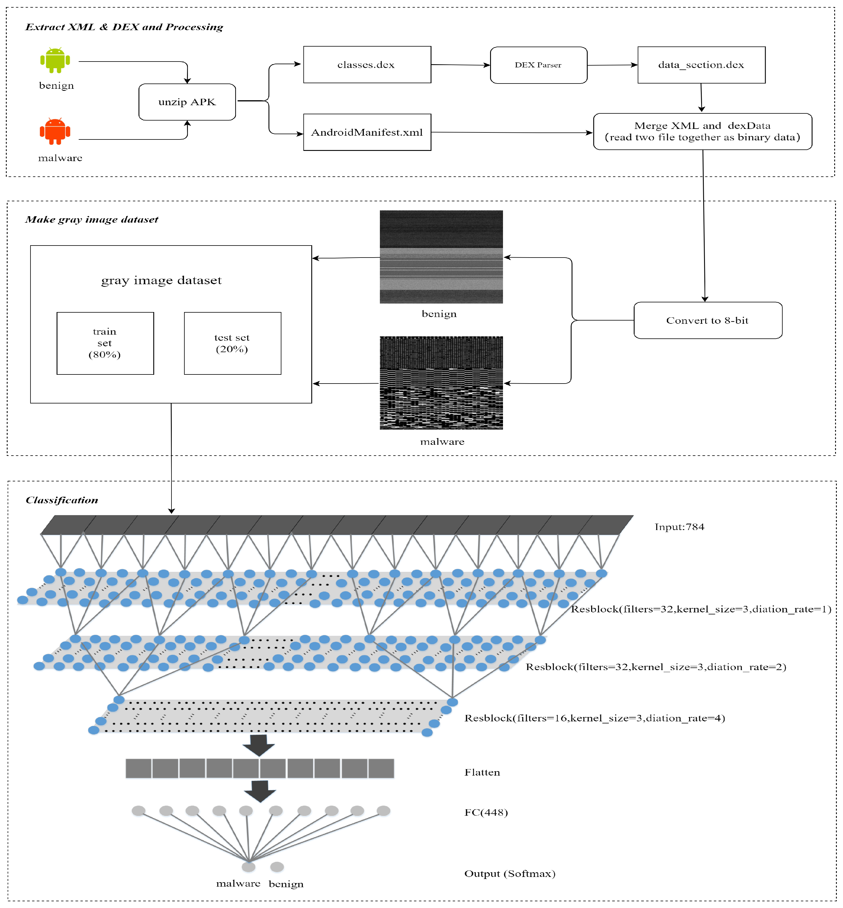
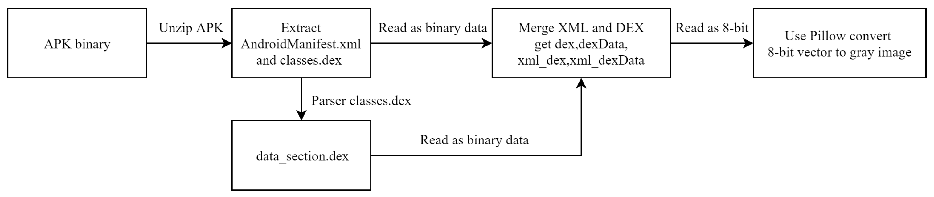
The method proposed in this paper is divided into three parts:

• Extract XML and DEX and processing:
  We extract AndroidManifest.xml and classes.dex from APK, decompiling the data section of classes.dex by using DEXparser. We save the DEX file data section as a data_section.dex file. Then, we merge AndroidManifest.xml and data_section.dex by reading them together as binary data;
• Make gray image dataset:
  The merged binary data is read as 8-bit vectors, then it is converted into gray-scale images with a unified size of 28 × 28. After being stored in the IDX format, the image data set is divided into a training set and test set, according to the ratio of 8:2;
• Classification:
  Finally, the classification module inputs the data set into our TCN model. We classify and verify the data set by using the tenfold crossvalidation method, and obtain the detection result by the Softmax method. Figure 1 shows an overview of our method.
  

  Figure 1. Android malware detection method overview.

3.2. APK File Structure

APK can be regarded as a compressed package file. After it is decompressed, it generally contains the following directories and files, as shown in Table 1 below:

Table 1. Structure of APK.

File or Directories	Function Description
assets	Store static files that need to be packaged into APK
META-INF	Store application signatures and certificates to ensure the integrity of APK packages and system security
res	All the resource files needed by the APK
libs	The library folder
AndroidManifesst.xml	The configuration file of the application program, which includes the name, version number, required permissions, registration service, linked other applications, declaration of the four components, and call information of the application program
classes.dex	The runnable file on the Dalvik virtual machine, which contains all the operating instructions of the application and runtime data
resources.ars	The compiled binary resource files

AndroidManifesst.xml contains permission information, which is the first line of defense for Android applications. Classes.dex is a very important file, and it is also the object that most security experts often analyze for Android malware at present. The structure of the DEX file is shown in Figure 2. We can extract the data area part of classes.dex, according to the data size and data offset contained in the header. Then, it is saved as data_section.dex.

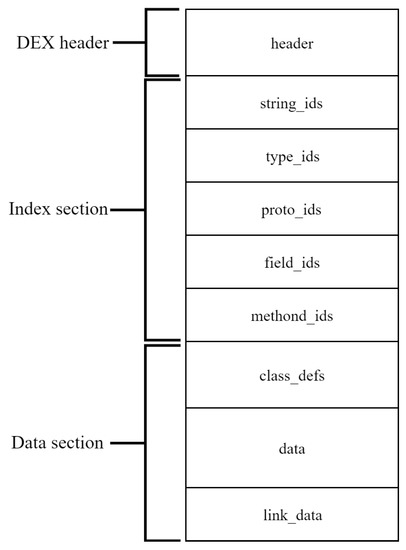
Figure 2. Structure of DEX file.

3.3. Visualization of Android APK File

The AndroidManifest.xml, classes.dex, data_section.dex files obtained by decompressing APK files can be read as vectors of 8bit unsigned integers. Then, the width of the generated image is determined according to the size of the files in Table 2. The vector size is divided by the width and the height of gray image. Finally, Pillow [27] is used to convert the 8bit vector into a gray image as shown in Figure 3 below:

Table 2. Image width for file sizes.

File Size Range	Image Width
<10 KB	32
10 KB~30 KB	64
30 KB~60 KB	128
100 KB~200 KB	384
200 KB~500 KB	512
500 KB~1000 KB	764
>1000 KB	1024

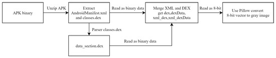
Figure 3. Visualizing XML and DEX files as gray images.

The following Algorithm 1 is the merge of AndroidManifest.xml and classes.dex files, and the xml_dexData gray image generation algorithm:

Algorithm 1 Gray image generation algorithm

Input: Binary file XML(AmdroidManifest.xml) and dexData(data_setcion.dex); Output: xml_dexData(gray_image); 1: xml_file_size ← get_file_size(XML); 2: dexData_file_size ← get_file_size(dexData); 3: merge_file_size ← xml_file_size + dexData_file_size; 4: width ← get_image_width(merge_file_size); 5: height ← dexData_file_size/width; 6: xml_array ← numpy.formfile(xml,dtype=numpy.unit8); 7: dex_array ← numpy.formfile(dexData,dtype=numpy.unit8); 8: xml_dexData_array ← numpy.append(image_xml,image_dex); 9: xml_dexData_array ← numpy.reshape(xml_dexData_array,(height,width)); 10: Gray image ← Pillow.Image.formarray(xml_dexdata_array); 11: return xml_dexData(gray image);

3.4. Experiment Features

In our experiment, there are four different features, divided by us. Two of them are combined features. The DEX image is obtained by directly visualizing classes.dex; the dexData image also is directly visualized from the data_section.dex file. The xml_dex image is visualized by combining classes.dex and AndroidManifest.xml. The xml_dexData image is visualized by combining AndroidManifest.xml and dex_section.dex.

Figure 4 shows four different gray images after visualization of an APK. The MD5 code of this APK is 000a067df9235aea987cd1e6b7768bcc1053e640b267c5b1f0deefc18be5dbe.

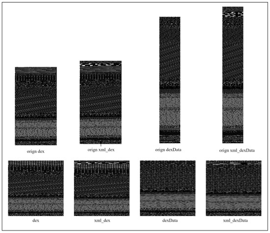
Figure 4. Gray image with four different feature combinations.

The original image is directly converted according to the file size, and below it is the image obtained after the uniform size is 28 × 28.

4. Malware Detection Introduction

In order to better evaluate the performance of different algorithms on the same data set, we implemented CNN, MobileNetV2 and TCN models to process data sets with four different feature combinations.

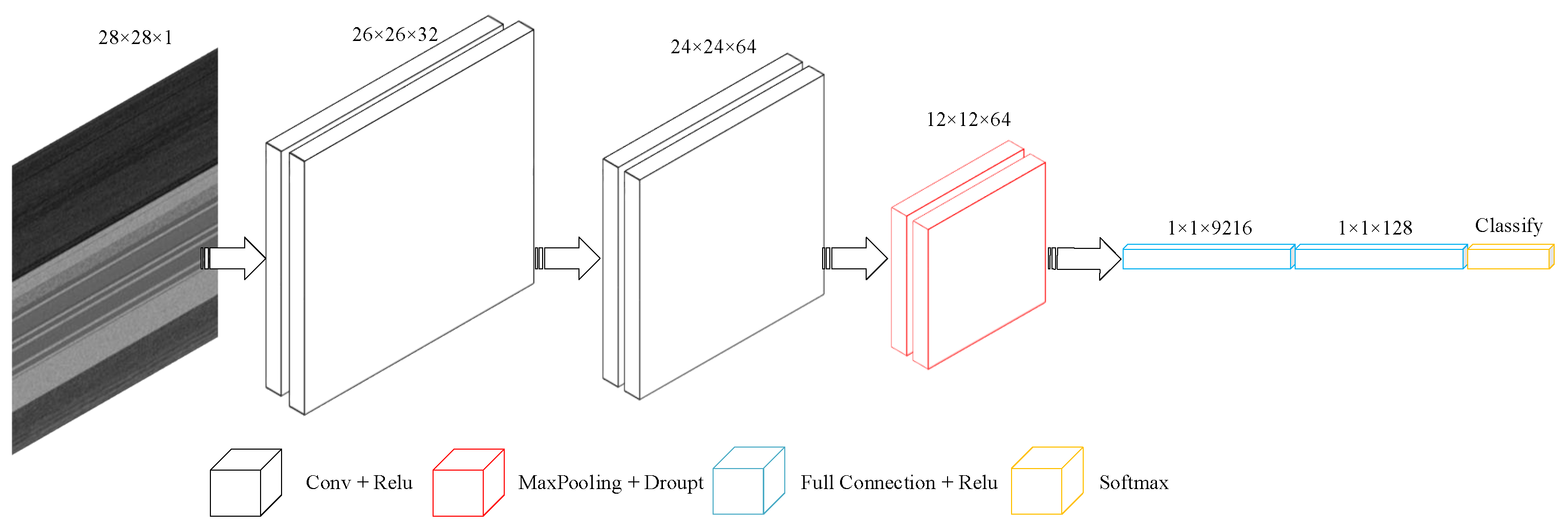
4.1. CNN Model

This is a baseline classification model designed by us to compare the influence of texture image feature combination of DEX, dexData, xml_dex, and xml_dexData on classification accuracy. The main architecture of the model is shown in the following Figure 5:

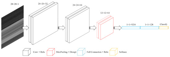
Figure 5. The classification structure of CNN.

The first convolution layer uses 32 convolution kernels with a kernel_size of (3,3). The second convolution layer uses 64 convolution kernels with a kernel_size of (3,3). The maximum pooling layer size of the third layer is (2,2), and the dropout parameter is 0.25. The dense layer parameter is 128. Finally, the Softmax function is used in the classification layer.

In the Softmax classification regression method, multi-category samples are classified by estimating the probability of the category to which the samples belong. Assuming that the training set is $x_i\in \left\{\left(x_1,y_1\right),\left(x_2,y_2\right),\cdots \left(x_m,y_m\right)\right\}$, the label data are $y_i\in \left\{1,2,\cdots k\right\}$. Then, for given test datum $x_i$, the probability distribution of its corresponding category label $y_i$ is as follows:

$$h_{\theta }(x^i)=\left[\begin{array}{c}p(x^i=1|x^i;\theta )\\ p(y^i=2|x^i;\theta )\\ ⋮\\ \mathrm{p}({\mathrm{y}}^i=k|x^i;\theta )\end{array}\right]=\frac{1}{\sum _{j=1}^k{e}^{{\theta }_j^T{x}^i}}\left[\begin{array}{c}{e}^{{\theta }_1^T{x}^i}\\ e^{{\theta }_2^T{x}^i}\\ ⋮\\ e^{{\theta }_k^T{x}^i}\end{array}\right]$$

(1)

where ${\theta }_1,{\theta }_1,\cdots {\theta }_k\in {}^{n+1}$ are the parameters of the model, and $\frac{1}{{\displaystyle \sum _{j=1}^k}{e}^{{\theta }_j^T{x}^i}}$ is a normalization of the probability distribution to ensure that the sum of all probabilities is 1.

4.2. MobileNetV2 Model

MobileNetV2 is a CNN model proposed by Marker Sander [28] for mobile device construction. MobileNetV2 introduces the residual structure based on the depth separable convolution of MobileNetv1. Because RELU has a very serious information loss problem in Feature Map with fewer channels, a linear bottleneck and inverted residual are added to solve it.

The depth separable convolution is different from the standard convolution, depth convolution and point convolution in the structure, thus generating different computations in corresponding convolution operations. In standard convolution, the number of channels in the convolution kernel needs to be equal to the number of channels in the input data. For example, for an input feature map with M channels, the convolution kernel size is $D_K$. We hope to get an output feature map with N channels and the size of the output feature map is $\left(D_W,D_H\right)$.

In the standard convolution, the computation of the one layer network is $D_W\times D_K\times M\times N\times D_W\times D_H$

The computational cost of depthwise convolution is $D_K\times D_K\times M\times D_W\times D_H$

The pointwise convolution computation is $M\times N\times D_W\times D_H$

The depth separable convolution computation is $D_K\times D_K\times M\times D_W\times D_H+M\times N\times D_W\times D_H$

The computational ratio of depth separable to traditional convolution is as follows:

$$\frac{D_K\times D_K\times M\times D_W\times D_H+M\times N\times D_W\times D_H}{D_K\times D_K\times M\times N\times D_W\times D_H}=\frac{1}{N}+\frac{1}{D_K^2}$$

(2)

Through the comparison of computation, it is found that depthwise separable convolution can solve the problem that the number of parameters and computation cost of traditional convolution are too high. Next, we introduce the network structure of MobileNetV2 used in this paper, which is mainly divided into a core structure and a network overview.

4.2.1. Core Architecture of MobileNetV2

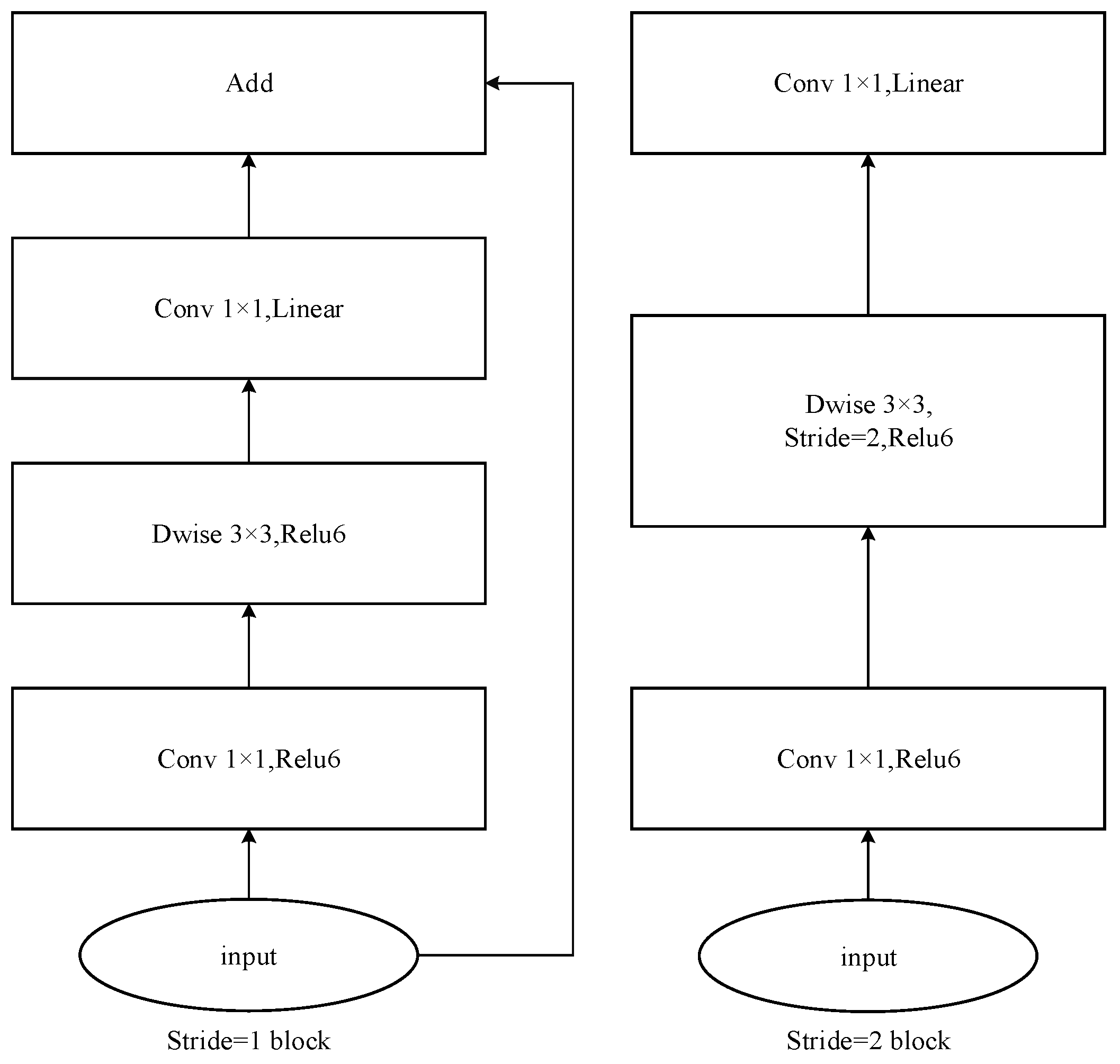
Inverted residuals and handstand residuals are used in MobileNetV2. It is different from the previous resident block, which compresses first, then convolves to extract features, and then expands. Inverted residuals first expand six times, then convolve to extract features, and finally compress and output features of this layer. When the ReLu activation function is used, some information will be lost. The addition of linear bottlenecks can play a role in preserving effective features. For stride = 1 and stride = 2, there is a slight difference in the block, mainly to match the dimension of shortcut. The purpose of shortcut is to solve the problems of gradient divergence and difficult training in deep networks. Therefore, when stride = 2, shortcut is not used. Figure 6 shows two basic bottleneck architectures for MobileNetV2:

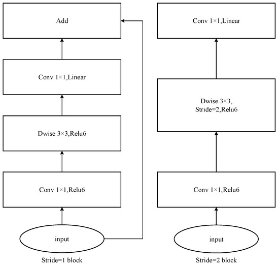
Figure 6. The core structure of MobileNetV2.

4.2.2. MobileNetV2 Network Architecture

We used the standard MobileNetv2 network architecture in our lab, as shown in Table 3.

Table 3. Network architecture of standard MobileNetV2.

Input	Operator	t	c	n	s
$224\times 224\times 3$	Conv2d	-	32	1	2
$112\times 112\times 32$	Bottleneck	1	16	1	1
$112\times 112\times 16$	Bottleneck	6	24	2	2
$56\times 56\times 24$	Bottleneck	6	32	3	2
$28\times 28\times 32$	Bottleneck	6	64	4	2
$14\times 14\times 64$	Bottleneck	6	96	3	1
$7\times 7\times 96$	Bottleneck	6	160	3	2
$7\times 7\times 320$	Conv2d $1\times 1$	-	1280	1	1
$7\times 7\times 1280$	Avgpool $7\times 7$	-	-	1	1
$1\times 1\times 1280$	Conv2d $1\times 1$	-	k	-	-

Here, t represents the expansion factor, c represents the number of output channels, n represents the number of repetitions, and s represents the step stride. The expansion factor t is used to adjust the size of the input image, as shown in Table 4:

Table 4. Application of expansion factor t.

Input	Operator	Output
$h\times w\times k$	$1\times 1$ Conv2d	$h\times w\times tk$
	ReLU6
$h\times w\times tk$	$3\times 3$ Dwise s = s	$\frac{h}{s}\times \frac{w}{s}\times tk$
	ReLU6
$\frac{h}{s}\times \frac{w}{s}\times tk$	Linear $1\times 1$	$\frac{h}{s}\times \frac{w}{s}\times k$

In the selection of the final classification function, we chose the Sigmod function because the Sigmod function is similar to the two-classification special case of the Softmax function. The Sigmod function formula is as follows:

$$\sigma \left(x\right)=\frac{1}{1+e^{-x}}$$

(3)

Assume the sample $x\in \left\{\left(x_1,y\right),\left(x_2,y\right),\cdots \left(x_i,y\right)\right\}$, and define the indicator function:

$$f_i\left(x,y\right)=\left\{\begin{array}{cc}x& \\ 0& \end{array}\begin{array}{c}\mathrm{y}=1\\ \mathrm{y}=0\end{array}\right.$$

(4)

According to the Sigmod formula, the probability of category 1 can be obtained as follows:

$$p\left(y=1|x\right)=\frac{1}{1+e^{-{\displaystyle \sum _i}{w}_{i}x}}$$

(5)

4.3. TCN Model

TCN was proposed by Shaojie Bai [29] to solve the problem of time series modeling. It was found that TCN can reach or even surpass the RNN model in many tasks. We read the image as 1-dimensional data, making TCN suitable for processing bytecode sequences with a sequential structure. The core structure of TCN is mainly composed of dilated convolution and residual connection. In the following two parts, we introduce the dilated convolution and residual connection used in our experiment.

4.3.1. Dilated Convolution

In the TCN model, causal convolution is introduced firstly. However, simple causal convolution still has the problem of a traditional convolution neural network. The problem is that the modeling length of events is limited by the size of the convolution kernel. In order to capture the dependencies of longer sequences, many layers need to be stacked linearly. In order to solve this problem, dilated convolution is added.

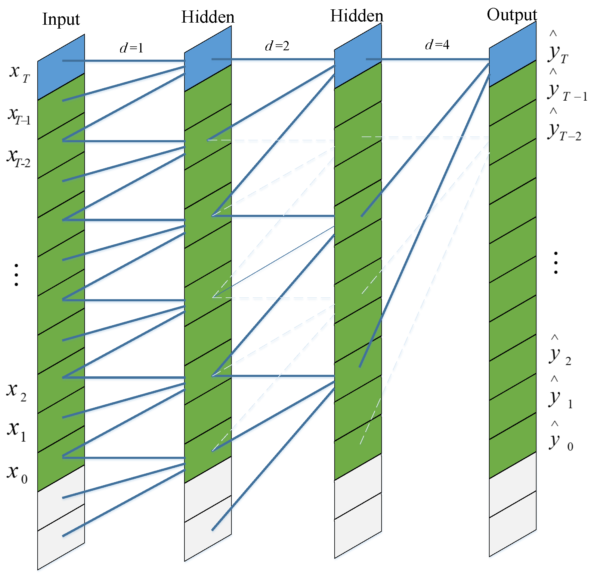
Assuming that, given an input sequence $x_0,x_1,x_2,\cdots ,x_{T-2},x_{T-1},x_T$. We hope that the output corresponding to the prediction $y_0,y_1,y_2,\cdots ,y_{T-2},y_{T-1},y_T$. The mapping function $f:X^{T+1}\to Y^{T+1}$ can be expressed as follows:

$${\widehat{y}}_0,{\widehat{y}}_1,{\widehat{y}}_2,\cdots ,{\widehat{y}}_{T-2},{\widehat{y}}_{T-1},{\widehat{y}}_T=f\left(x_0,x_1,x_2,\cdots ,x_{T-2},x_{T-1},x_T\right)$$

(6)

The schematic diagram of the prediction process for the input sequence is shown in Figure 7. Different from traditional convolution, the input of dilated convolution has interval sampling. The sampling interval is determined by the dilation factor d. When $d=1$ between input and hidden, this means that each point is sampled at the input. The middle layer $d=2$ indicates that every two points are sampled as one input at the time of input. When $d=4$, this means sampling every 4 points as the output. Typically, as the network layers increase, the value of d also needs to increase. In this way, the convolution network can obtain a large receptive field with a relatively small number of layers.

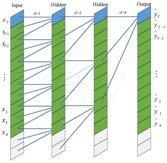
Figure 7. Dialted convolution of TCN model.

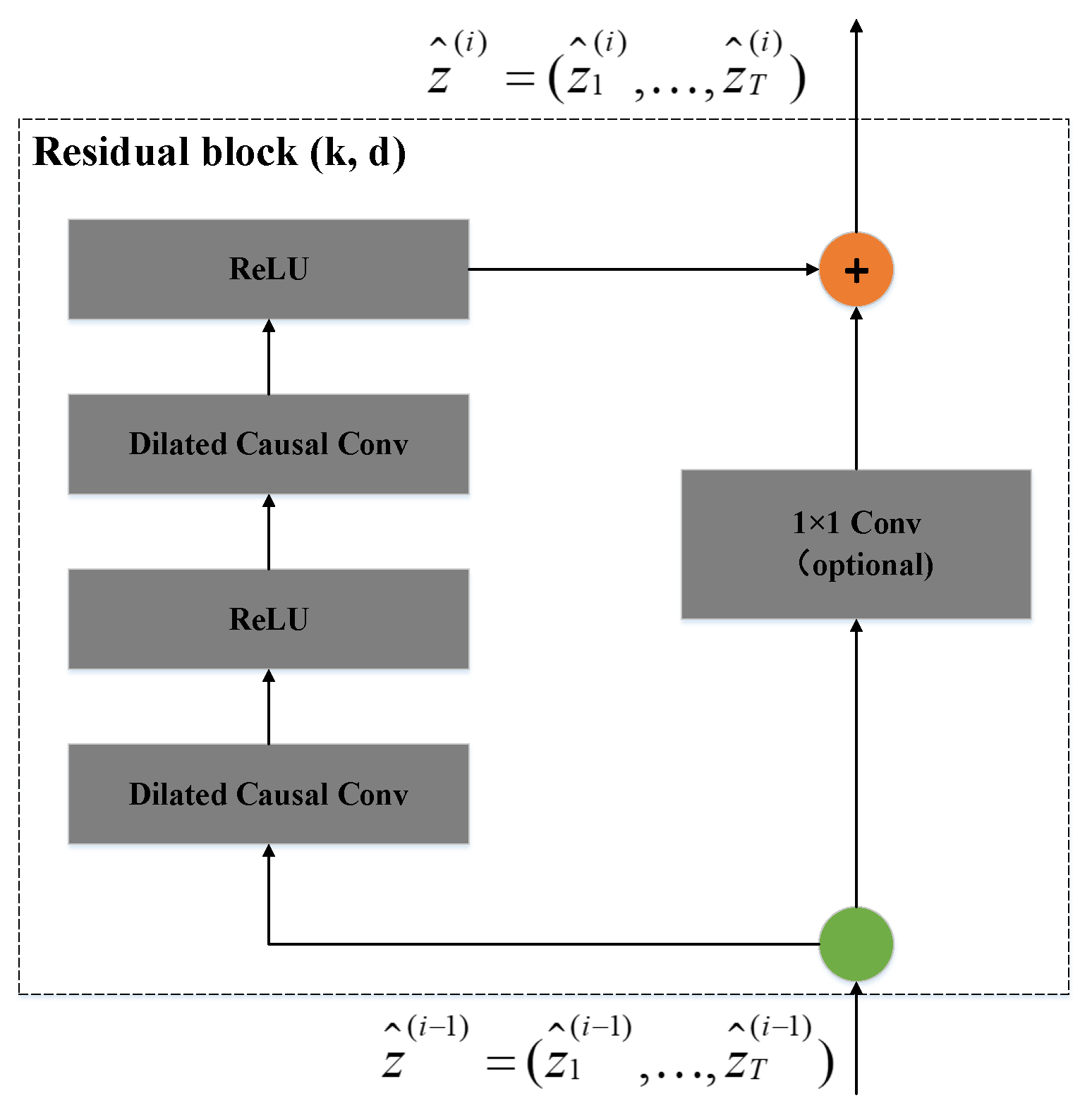
4.3.2. Residual Connection

Residual connection is an effective method to train a deep network, which can make the network transmit information in a cross-layer way. The residual module we implemented is different from the residual module in the standard TCN, without adding Dropout and WeightNorm layers.

In Figure 8, ${\widehat{z}}^{(i-1)}$ represents the input of the residual block, and ${\widehat{z}}^{\left(i\right)}$ represents the output of the residual block. In the final classification function selection, we used the probability score output by the Softmax function to obtain the prediction result, like the CNN before.

Figure 8. Residual block of TCN model.

5. Experiment

5.1. Experiment Conditions

The experimental environment is based on the Python [30] version 3.6.5, Anaconda integrated environment. All models are implemented using Tensorflow [31] version 1.14 and Keras [32] version 2.25. The experiment was carried out on a Windows system with Intel xeon CPU E5-2650 V4 with 2.20 GHZ.

5.2. Dataset

The data in this experiment come from the Canadian Institute for Cybersecurity [33], which is composed of three data sets: CICANdMal2017, CICInvesAndMal2019 and CICMalDroid 2020. The CICInvesAndMal2019 data set is the second part of the CICANdMal2017 data set. We sorted out and removed duplicate data, and selected 11,513 benign and malicious samples for the experiment. The data sets’ distribution is shown in Table 5.

Table 5. Data set distribution.

Samples	Type and Number	Source
	Adware (1104)
	Ransomware (101)	CICAndMal2017
malware (5826)	Scareware (112)	CICInvesAndMal2019
	SMSmalware (1680)	CICMalDroid2020
	Banking (1190)
benign (5687)	Google Play (5687)

After converting the bytecode file of APK into a gray image data set, it is stored in IDX format of which 80% is used as a training set and 20% is used as a test set.

5.3. Evaluation Metrics

In order to measure the effectiveness of our proposed Android malware detection model, the detection results are expressed by a confusion matrix.

As show in Table 6, true positive (TP) is the number of benign APKs correctly predicted as benign APKs. True negative (TN) is the number of malicious APKs correctly predicted as malicious APKs. False positive (FP) is the number of malicious APKs that are wrongly predicted as benign APKs. False negative (FN) is the number of positive APK errors predicted as malicious APK.

Table 6. Confusion matrix.

	Predict	Benign	Malware
Actual
benign		TP	FN
malware		FP	TN

There are four evaluation metrics to evaluate the performance of our model: accuracy, precision, recall and F1-score.

Accuracy represents the ability of the model to correctly detect benign and malicious APKs. The calculation formula is as follows:

$$accuracy=\frac{TP+TN}{TP+FP+FN+TN}$$

(7)

Precision represents the proportion of the actual benign APK in the model-predicted benign APK. The calculation formula is as follows:

$$precision=\frac{TP}{TP+FP}$$

(8)

Recall represents the proportion of the model that correctly predicts the benign APK in the number of results predicted by the benign APK. The calculation formula is as follows:

$$recall=\frac{TP}{TP+FN}$$

(9)

The F1-score represents the reconciled average of precision and recall. The calculation formula is as follows:

$$\mathrm{F}1-\mathrm{score}=2\times \frac{precision\times recall}{precision+recall}$$

(10)

5.4. Model Training and Result Analysis

In order to better compare the performance of different algorithms on the same data set, we implemented three convolution neural network models: CNN, MobileNetV2 and TCN. These three models were used to carry out experiments on four different datasets. Then, we compared and analyzed which algorithm and feature combination are more suitable for Android malware detection.

5.4.1. CNN (Base Model)

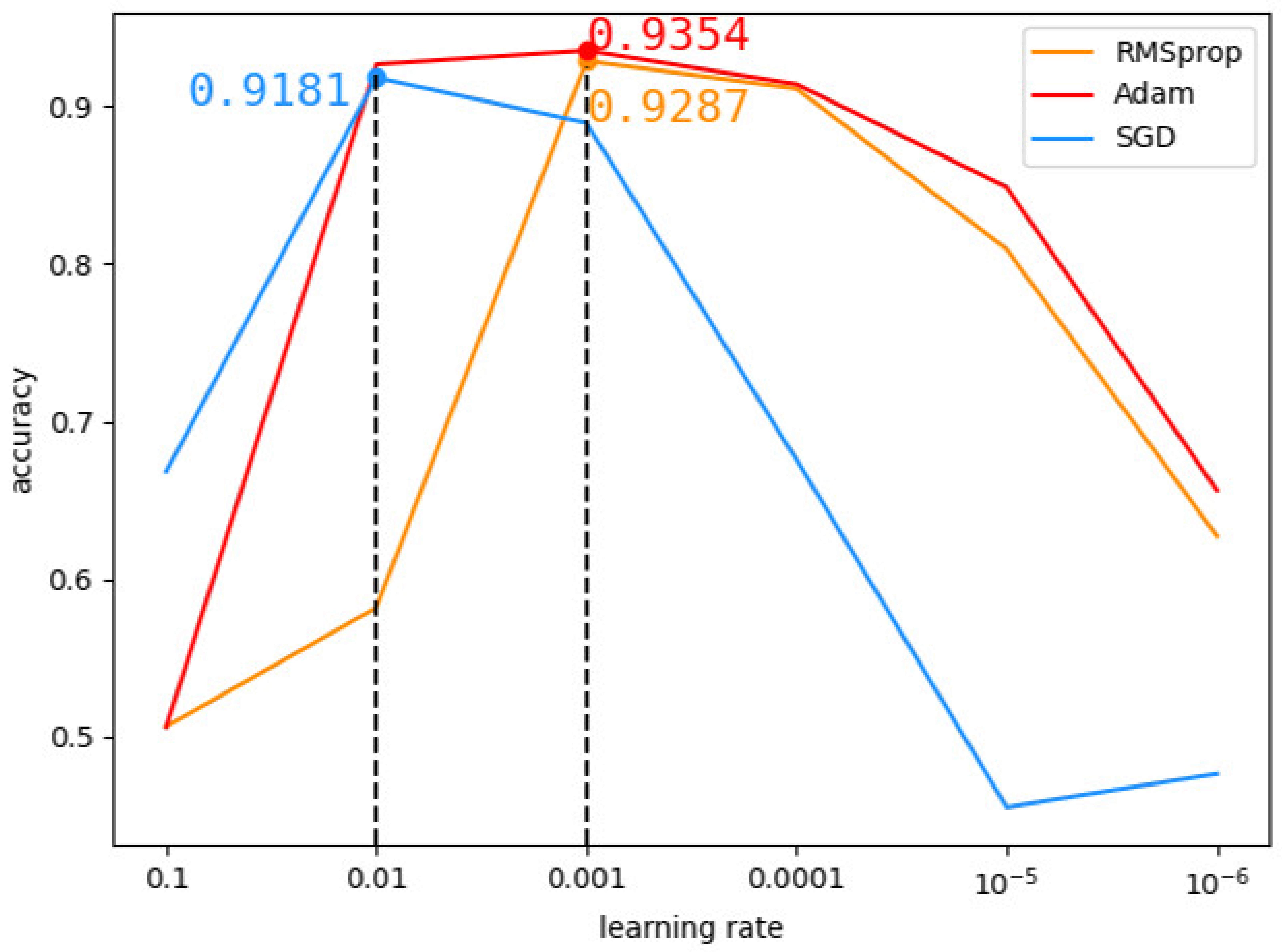
We analyzed the influence of Adam, RMSProp and SGD optimizers on the CNN model with the DEX data set. Firstly, the learning rate was set to 0.1, 0.01, 0.001, 0.0001, 0.00001 and 0.000001 respectively to observe the change in model accuracy. As shown in Figure 9, Adam optimizer was found to have the highest accuracy between 0.001 and 0.01. Finally, the learning rate in Adam optimizer was tested from 0.001 to 0.01, and Figure 10 shows that the optimal learning rate is 0.003.

Figure 9. Comparison of different optimizers.

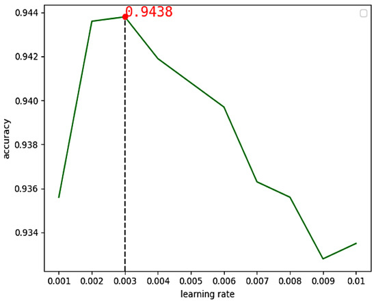
Figure 10. The accuracy of CNN changes with learning rates between 0.001 and 0.01.

Therefore, the final super parameter setting of CNN model in our experiment is learning rate = 0.003, batch_size = 128, epochs = 40. We used a ten-fold cross validation method to experiment on the training set. Referring to reference [13], using earlystopping can prevent the model from being over-fitted. We used earlystopping in Keras to monitor the accuracy changes of the validation set in 5 epochs and selected the optimal training model. The final experimental results are shown in Table 7 below:

Table 7. CNN model detection result metrics in four data sets.

Data Set	Accuracy	Precision	Recall	F1-Score
dex	0.9404	0.9407	0.9403	0.9404
xml_dex	0.9411	0.9411	0.9410	0.9410
dexData	0.9457	0.9459	0.9457	0.9456
xml_dexData	0.9470	0.9474	0.9470	0.9470

From Table 7, we can see that the accuracy of the xml_dex image feature data set on CNN model is 0.07% higher than that of the DEX image feature data set, and the accuracy of the xml_dexData image feature data set on CNN is slightly higher, 0.13%, than that of the dexData image feature data set. CNN performs best on xml_dexData image feature dataset. It is preliminarily confirmed that our addition of XML visualization features is conducive to Android malware detection.

5.4.2. MobileNetV2

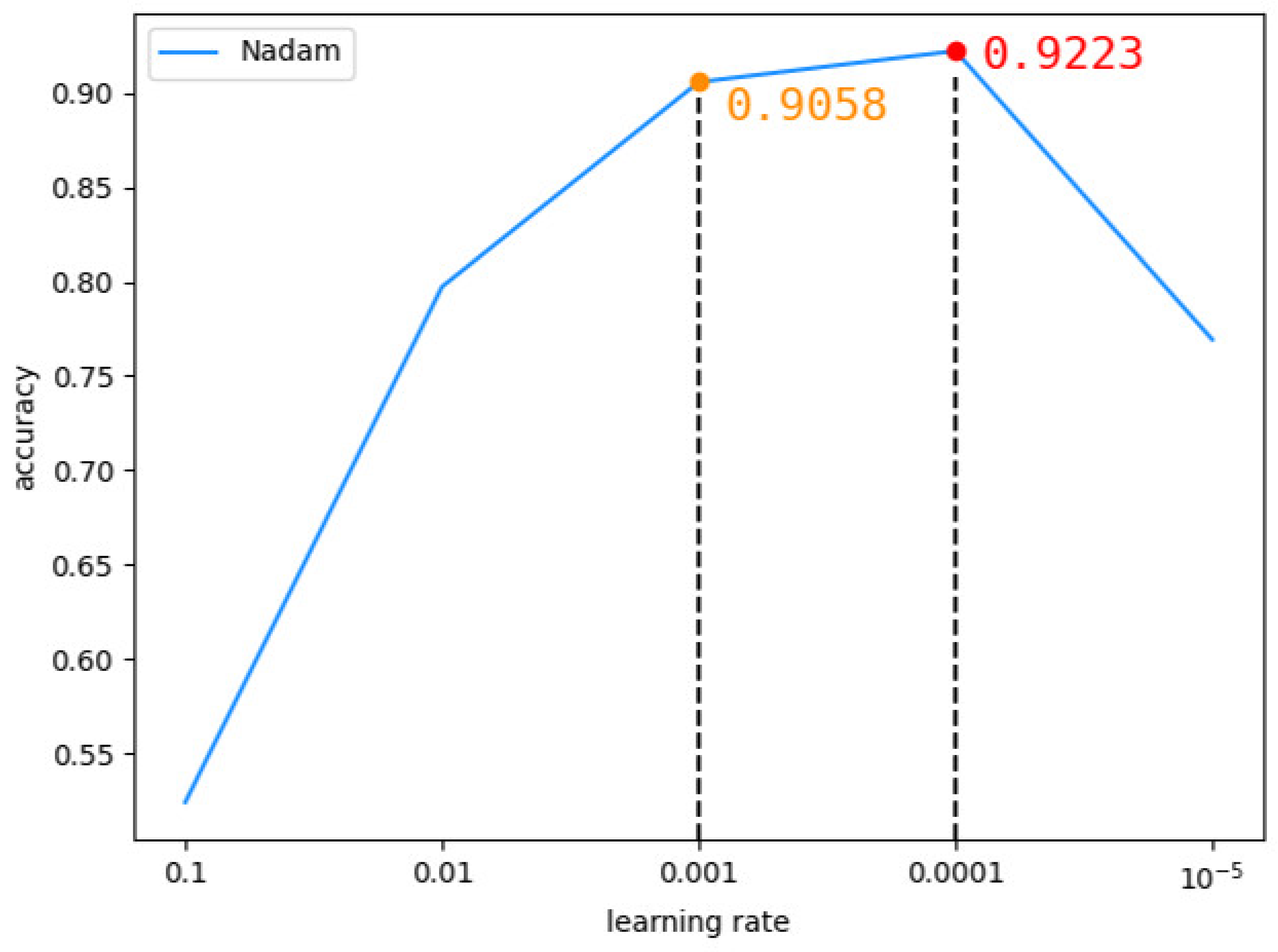
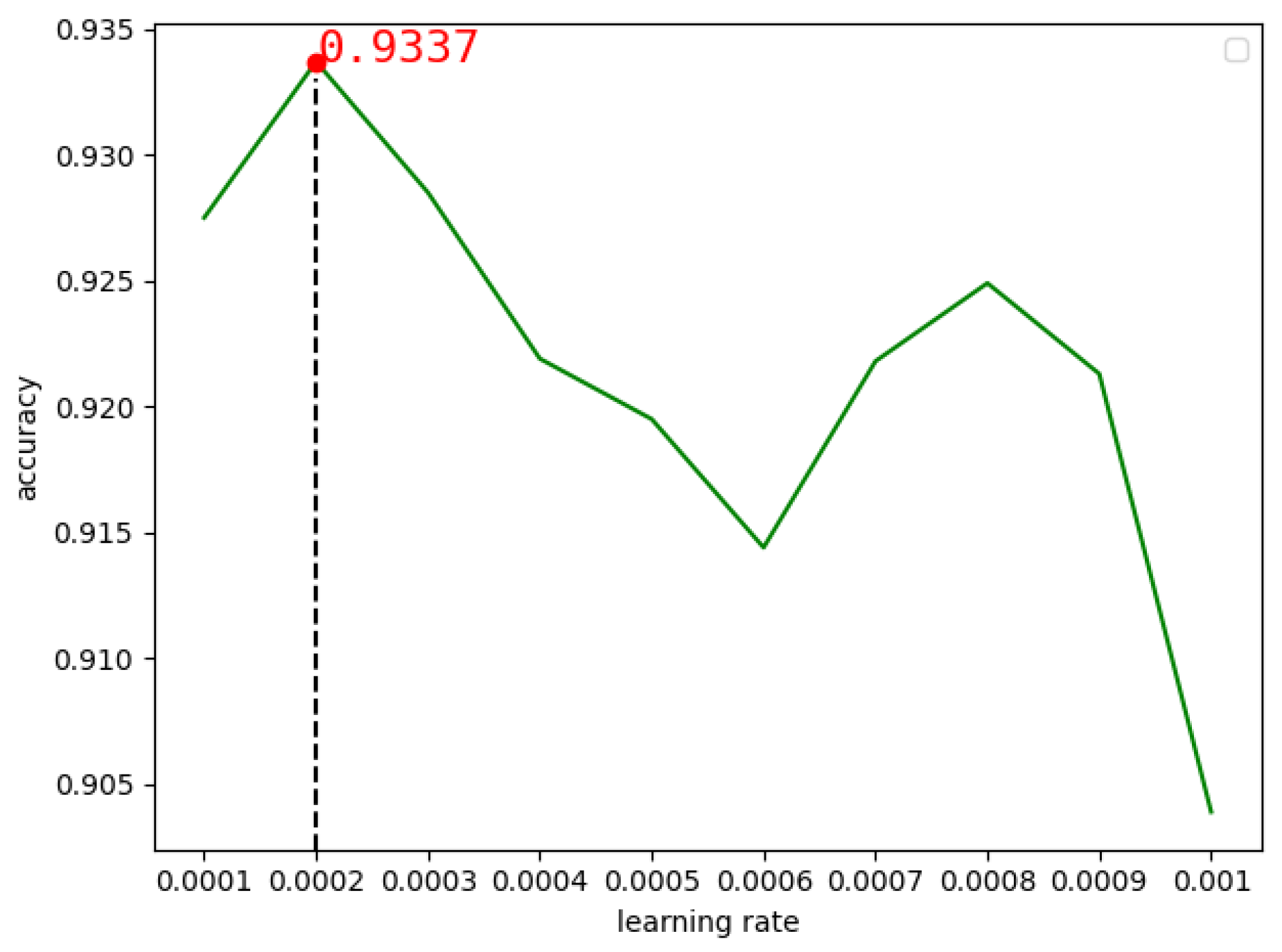
In the MobileNetV2 model, we chose to use the Nadam optimizer with the DEX data set. Firstly, the learning rate was set to 0.1, 0.01, 0.001, 0.0001 and 0.00001 respectively to observe the change of model accuracy. It was found that when the learning rate was 0.001, the accuracy rate of the model was 0.9058, and when the learning rate was 0.0001, the accuracy rate was 0.9223, as shown in Figure 11 below. Therefore, we conducted experiments between 0.0001 and 0.001, and found that when the learning rate was 0.0002, the highest accuracy rate was 0.9337, as shown in Figure 12 below.

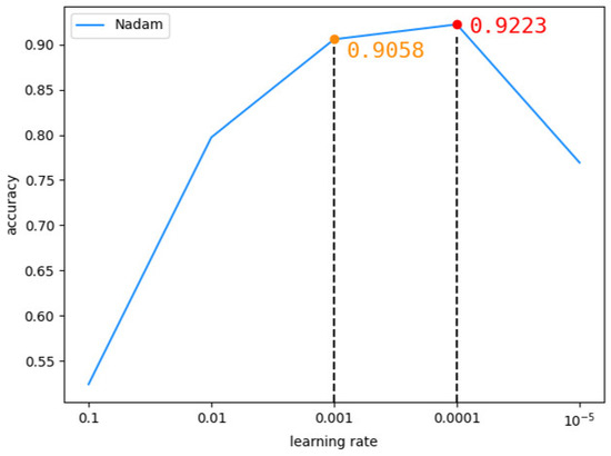
Figure 11. The accuracy of MobileNetV2 changes with learning rates between 0.00001 and 0.1.

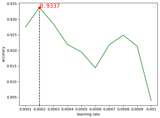
Figure 12. The accuracy of MobileNetV2 changes with learning rates between 0.0001 and 0.001.

Therefore, the super parameters in the experiment were set as follows: learning rate = 0.0002, batch_size = 128, epochs = 40. The experiment was carried out through 10-fold cross-validation, and earlystopping was also used to monitor the accuracy of every 5 epochs to avoid over-fitting. The final experimental results are shown in Table 8 below:

Table 8. MobileNetV2 model detection result metrics in four data sets.

Data Set	Accuracy	Precision	Recall	F1-Score
dex	0.9484	0.9484	0.9483	0.9483
xml_dex	0.9489	0.9490	0.9490	0.9489
dexData	0.9482	0.9483	0.9482	0.9482
xml_dexData	0.9506	0.9506	0.9505	0.9505

As can be seen from Table 8, the accuracy of the xml_dex image feature dataset on MobileNetV2 model is 0.05% higher than that of the DEX image feature dataset. The accuracy of the xml_dexData image feature data set on the MobileNetV2 model is also slightly higher than that of the dexData image feature data set, by 0.24%. MobileNetV2 also has the highest accuracy on xml_dexData image feature data set, which further confirms that visual XML features are conducive to Android malware detection.

5.4.3. TCN

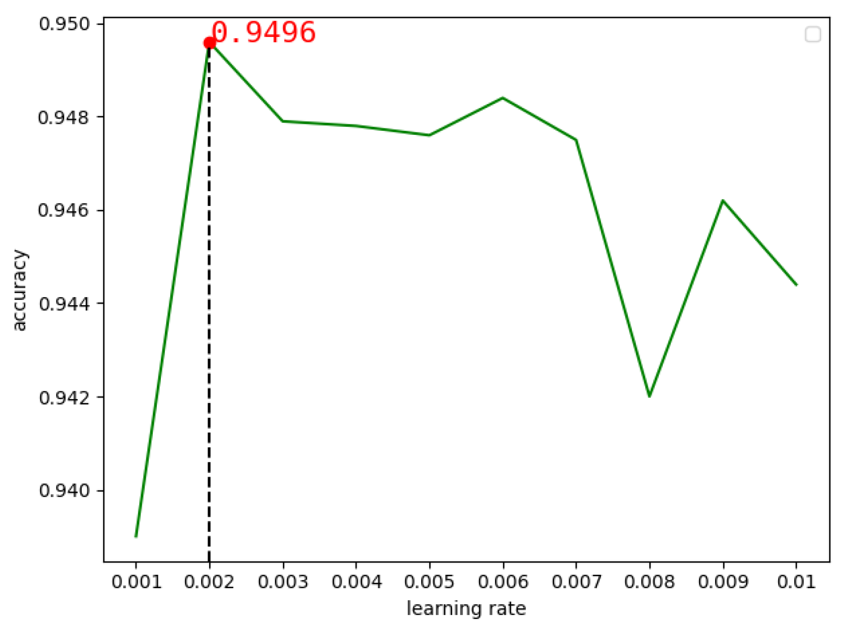
In the TCN model, we chose the Adam optimizer for experiments of the DEX dataset. The learning rate was set to 0.1, 0.01, 0.001, 0.0001 and 0.00001 respectively. Figure 13 shows that when the learning rate is 0.01, the accuracy rate is 0.9444, and when the learning rate is 0.001, the accuracy rate is 0.9459. We found that in the interval [0.01,0.001], the accuracy rate was the highest, so we continued to look for the optimal learning rate in this interval. As can be seen from Figure 14, when the learning rate is 0.002, the highest accuracy rate is 0.9496.

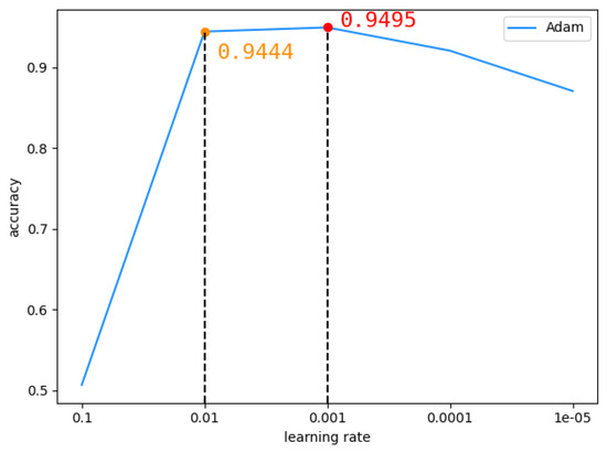
Figure 13. The accuracy of TCN changes with learning rates between 0.00001 and 0.1.

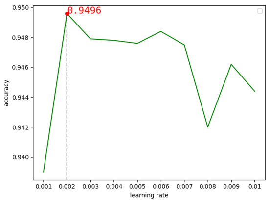
Figure 14. The accuracy of TCN changes with learning rates between 0.001 and 0.001.

So the super parameters we used for the experiment were learning rate = 0.002, batch_size = 128, and epochs = 40. The experiment was carried out through ten-fold cross-validation, and Keras earlystopping was used to monitor the accuracy changes of every 5 epochs to avoid over-fitting. We obtained the final experimental results as shown in Table 9.

Table 9. TCN model detection result metrics in four data sets.

Data Set	Accuracy	Precision	Recall	F1-Score
dex	0.9499	0.9499	0.9499	0.9499
xml_dex	0.9524	0.9526	0.9524	0.9524
dexData	0.9517	0.9518	0.9518	0.9517
xml_dexData	0.9544	0.9545	0.9545	0.9544

As can be seen from Table 9, the accuracy of xml_dex image feature data set on the TCN model is 0.25% higher than that of the DEX image feature data set. The accuracy of the xml_dexData image feature data set in TCN is also slightly higher than that of the dexData image feature data set by 0.27%. Consistent with the results of CNN and MobileNetV2 models in the experiment, the evaluation results of the xml_dexData image feature dataset on TCN are higher than those of the other three image feature data sets.

5.4.4. Result and Analysis

By comparing and verifying the experimental results of the above three models, we can find that after adding the visual features of AndroidManifest.xml file, the detection capability of Android malware is slightly improved. Moreover, our method can avoid the situation that the existing malware mainly relies on the visual features of DEX files, which is conducive to a more comprehensive detection of Android malware. Therefore, we recommend that xml_dexData is selected as the feature of Android malware detection. The evaluation results of CNN, MobileNetV2 and TCN for the xml_dexData data set are compared as shown in the following Table 10.

Table 10. Results comparison of different methods.

Method	Accuracy	Precision	Recall	F1-Score
CNN	0.9470	0.9474	0.9470	0.9470
MobileNetV2	0.9506	0.9506	0.9505	0.9505
TCN	0.9544	0.9545	0.9545	0.9544

We can see that TCN model has higher accuracy, precision, recall and F1-score than CNN and the MobileNetV2 models. Different from CNN and MobileNetV2, which process two-dimensional data as input, TCN processes one-dimensional sequence data as input. Because our visualization process of bytecodes is reading directly in bytecode order, one-dimensional sequence data are more suitable for extracting the sequence feature distribution of XML files and DEX files. Moreover, TCN itself is suitable for processing data with time series characteristics, and can capture similar information of fixed lengths by using its causal convolution characteristics. From the experiment, we know that TCN model can make full use of the sequence information in XML file, and has a good ability to detect Android malware.

We also compared the calculation parameters and time consumption of the three models in the experiment, as shown in Table 11.

Table 11. Effect Comparison of Different Models.

Model	Parameters	Training Times/Epochs	Accuracy
CNN	1,198,850	9.63 s	0.9470
MobileNetV2	2,278,210	44.76 s	0.9506
TCN	19,538	1.08 s	0.9544

The CNN model designed in our experiment generates more computations due to the traditional convolution method. MobileNetV2, as a lightweight convolution neural network, uses a deep separable convolution method, which can reduce the complexity and computation of the model. Because MobileNetV2 model is a deep neural network compared with the CNN model and TCN model, its training time is relatively long in the experiment.

Compared with the other two models, the TCN model has the fewest number of parameters and the least training time, and the accuracy of Android malware detection is the highest. This is because the residual module of the TCN model has 1 × 1 convolution, which can reduce the calculation amount of the model. The input of the TCN model is to process bytecode images as one-dimensional sequence data, which also confirms that the TCN model we built is suitable for Android malware detection. Compared with the traditional method, it can improve the detection rate of Android malware and, at the same time, reduce the computation and training time.

In order to better demonstrate the performance of the TCN model in Android malware detection, we compare it with the detection methods in the last four years. As shown in Table 12, the accuracy of GIST + RF [14] and CNN [32] is very close to ours, but the two methods have fewer samples and do not have their own open source data sets. Moreover, GIST + RF needs to use the GIST method to extract bytecode image features separately, which is more complicated than the CNN method. Although R2-D2 [23] uses large data sets, it does not use multiple evaluation metrics, and the accuracy rate is 2.44% lower than ours. CNN [16] uses the same magnitude data and the same evaluation metrics as our model, so we made a comprehensive comparison with it. This shows that the fusion of XML visualization features and DEX data section visualization features can be used as an effective feature for Android malware detection. The TCN model we built can effectively utilize visual sequence features, and the detection accuracy of Android malware exceeds that of traditional CNN methods and machine learning methods.

Table 12. The results of comparing the TCN and existing method.

Year	Method	Samples	Accuracy	Precison	Recall	F1-Score
2017	GIST+RF [15]	1280	95.42%	—	—	—
2018	R2-D2 [25]	829,356	93%	—	—	—
2019	CNN [18]	10,440	93%	93.6%	94.4%	94.0%
2020	CNN [34]	4962	95.1%	—	—	—
2021	TCN	11,513	95.44%	95.45%	95.45%	95.44%

6. Conclusions

In this paper, we used an image-based analysis method to avoid the malicious applications, which may have symmetric encryption, and confusion of the traditional static analysis process. The AndroidManifest.xml binary file feature and dex_section.dex binary file feature were fused together as Android malware visual features for the first time, and we proposed a new Android malware detection model based on TCN. Firstly, XML files and two DEX files were directly read and fused with binary data to create gray image data sets with different feature combinations. Then, experiments were carried out by using two-dimensional CNN and MobileNetV2 to analyze the differences of the four feature combinations. We found that adding visual features of XML files can reduce the dependence of the malware detection model on single DEX file features. We verified the reliability of the experiment by the ten-fold cross-validation method. MobileNetV2 can effectively reduce the computational complexity by using depth-separable convolution, but the network depth is too deep and cannot improve the accuracy of Android malware detection. However, 1 × 1 convolution is used in the residual module of TCN model, which can reduce the calculation amount of the model. The experimental results also showed that the TCN model has the least computation, the shortest average training time and the highest accuracy, compared with the other two models. Therefore, it is proved that the TCN model can be effectively applied to Android malware detection. On the other hand, the lightweight model in this paper can be deployed on Android mobile devices in the form of design APIs, as it takes up less storage resources.

TCN is a variant of the convolution neural network. Although the receptive field can be expanded by using extended convolution, it is still limited. We will explore the application of visual attention mechanisms to bytecode images to capture relevant information of any length in the future. More work in the future will entail conducting more in-depth analyses and research on XML files, improving the accuracy of Android malware detection, and embedding the improved model into mobile devices for use.

References

- National Internet Emergency Center. Overview of China’s Internet Network Security Situation in 2019. Available online: https://www.cert.org.cn/publish/main/46/2020/20200811124544754595627/20200811124544754595627_.html (accessed on 1 October 2020).
- Google Play Protect. 2018. Android. Available online: https://www.android.com/play-protect/ (accessed on 15 August 2020).
- Android’s Built-In Google Play Protect Protection Is Useless. Available online: https://www.cnbeta.com/articles/tech/759727.htm (accessed on 20 August 2020).
- Naway, A.; Li, Y. A Review on The Use of Deep Learning in Android Malware Detection. arXiv 2020, arXiv:1812.10360. [Google Scholar]
- Ganesh, M.; Pednekar, P.; Prabhuswamy, P.; Nair, D.S.; Park, Y.; Jeon, H. CNN-based android malware detection. In Proceedings of the 2017 International Conference on Software Security and Assurance (ICSSA), Altoona, PA, USA, 24–25 July 2017; pp. 60–65. [Google Scholar]
- Ding, Y.; Zhao, W.; Wang, Z.; Wang, L. Automaticlly Learning Featurs Of Android Apps Using CNN. In Proceedings of the 2018 International Conference on Machine Learning and Cybernetics (ICMLC), Chengdu, China, 15–18 July 2018; pp. 331–336. [Google Scholar]
- McLaughlin, N.; del Rincon, J.M.; Kang, B.; Yerima, S.; Miller, P.; Sezer, S.; Safaei, Y.; Trickel, E.; Zhao, Z.; Doupé, A.; et al. Deep Android Malware Detection. In Proceedings of the Seventh ACM on Conference on Data and Application Security and Privacy—CODASPY ’17, Scottsdale, AZ, USA, 22–24 March 2017; pp. 301–308. [Google Scholar]
- Salah, A.; Shalabi, E.; Khedr, W. A Lightweight Android Malware Classifier Using Novel Feature Selection Methods. Symmetry 2020, 12, 858. [Google Scholar] [CrossRef]
- Wang, X.; Yang, Y.; Zeng, Y. Accurate mobile malware detection and classification in the cloud. Springerplus 2015, 4, 1–23. [Google Scholar] [CrossRef] [PubMed] [Green Version]
- Afonso, V.M.; de Amorim, M.F.; Grégio, A.R.A.; Junquera, G.B.; de Geus, P.L. Identifying Android malware using dynamically obtained features. J. Comput. Virol. Hack. Tech. 2015, 11, 9–17. [Google Scholar] [CrossRef]
- Bagheri, H.; Sadeghi, A.; Jabbarvand, R.; Malek, S. Practical, Formal Synthesis and Automatic Enforcement of Security Policies for Android. In Proceedings of the 2016 46th Annual IEEE/IFIP International Conference on Dependable Systems and Networks (DSN), Toulouse, France, 28 June–1 July 2016; pp. 514–525. [Google Scholar]
- Arshad, S.; Shah, M.A.; Wahid, A.; Mehmood, A.; Song, H.; Yu, H. SAMADroid: A novel 3-level hybrid malware detection model for Android operating system. IEEE Access 2018, 6, 4321–4339. [Google Scholar] [CrossRef]
- Kouliaridis, V.; Kambourakis, G.; Geneiatakis, D.; Potha, N. Two Anatomists Are Better than One—Dual-Level Android Malware Detection. Symmetry 2020, 12, 1128. [Google Scholar] [CrossRef]
- Spreitzenbarth, M.; Schreck, T.; Echtler, F.; Arp, D.; Hoffmann, J. Mobile-sandbox: Combining static and dynamic analysis with machine-learning techniques. Int. J. Inf. Secur. 2015, 14, 141–153. [Google Scholar] [CrossRef]
- Manzhi, Y.; Qiaoyan, W. Detecting android malware by applying classification techniques on images patterns. In Proceedings of the 2017 IEEE 2nd International Conference on Cloud Computing and Big Data Analysis (ICCCBDA), Chengdu, China, 28–30 April 2017; p. 344347. [Google Scholar]
- Orralba, A.; Murphy, K.P.; Freeman, W.T.; Rubin, M.A. Context-based vision systems for place and object recognition. In Proceedings of the International Conference on Computer Vision (ICCV), Nice, France, 13–16 October 2003. [Google Scholar]
- Oliva, A.; Torralba, A. Modeling the shape of a scene: A holistic representation of the spatial envelope. Int. J. Comput. Vis. 2001, 42, 145–175. [Google Scholar] [CrossRef]
- Xiao, X. An Image-Inspired and CNN-Based Android Malware Detection Approach. In Proceedings of the 2019 34th IEEEACM International Conference on Automated Software Engineering (ASE), San Diego, CA, USA, 11–15 November 2019; pp. 1259–1261. [Google Scholar]
- Radanliev, P.; De Roure, D.C.; Nurse, J.R.C.; Montalvo, R.M.; Cannady, S.; Santos, O.; Maddox, L.; Burnap, P.; Maple, C. Future developments in standardisation of cyber risk in the Internet of Things (IoT). SN Appl. Sci. 2020, 2, 169. [Google Scholar] [CrossRef] [Green Version]
- Dexparser (Pil Fork). Available online: https://pypi.org/project/dexparser/0.0.1/ (accessed on 20 November 2020).
- Nataraj, L.; Karthikeyan, S.; Jacob, G.; Manjunath, B. Malware images: Visualization and automatic classification. In Proceedings of the 8th International Symposium on Visualization for Cyber Security, VizSec’11, Pittsburgh, PA, USA, 20 July 2011. [Google Scholar]
- Jung, D.-S.; Lee, S.-J.; Euom, I.-C. ImageDetox: Method for the Neutralization of Malicious Code Hidden in Image Files. Symmetry 2020, 12, 1621. [Google Scholar] [CrossRef]
- Kumar, A.; Sagar, K.P.; Kuppusamy, K.S.; Aghila, G. Machine learning based malware classification for Android applications using multimodal image representations. In Proceedings of the 2016 10th International Conference on Intelligent Systems and Control (ISCO), Coimbatore, India, 7–8 January 2016; p. 16. [Google Scholar]
- Darus, F.M.; Ahmad, S.N.A.; Ariffin, A.F.M. Android Malware Detection Using Machine Learning on Image Patterns. In Proceedings of the 2018 Cyber Resilience Conference (CRC), Putrajaya, Malaysia, 13–15 November 2018; p. 12. [Google Scholar]
- Huang, T.H.; Kao, H. R2-D2: ColoR-inspired Convolutional NeuRal Network (CNN)-based AndroiD Malware Detections. In Proceedings of the 2018 IEEE International Conference on Big Data (Big Data), Seattle, WA, USA, 10–13 December 2018; pp. 2633–2642. [Google Scholar]
- Jung, I.; Choi, J.; Cho, S.; Han, S.; Park, M.; Hwang, Y.-S. Android malware detection using convolutional neural networks and data section images. In Proceedings of the 2018 Conference on Research in Adaptive and Convergent Systems, Honolulu, HI, USA, 9–12 October 2018; pp. 149–153. [Google Scholar]
- Pillow (Pil Fork). Available online: https://pillow.readthedocs.io/en/stable/index.html (accessed on 1 October 2020).
- Sandler, M.; Howard, A.; Zhu, M.; Zhmoginov, A.; Chen, L.-C. MobileNetV2: Inverted Residuals and Linear Bottlenecks. In Proceedings of the IEEE Conference on Computer Vision and Pattern Recognition (CVPR), Salt Lake City, UT, USA, 18–23 June 2018; pp. 4510–4520. [Google Scholar]
- Bai, S.; Kolter, J.Z. Vladlen Koltun: An Empirical Evaluation of Generic Convolutional and Recurrent Networks for Sequence Modeling. arXiv 2018, arXiv:1803.01271. [Google Scholar]
- Python. Available online: https://www.python.org/ (accessed on 20 January 2020).
- TensorFlow. Available online: https://www.tensorflow.org/ (accessed on 20 January 2020).
- Keras. Available online: https://keras.io/ (accessed on 1 January 2020).
- Canandian Institute for Cybersecurity. Available online: https://www.unb.ca/cic/datasets (accessed on 20 January 2020).
- Ding, Y.; Zhang, X.; Hu, J.; Xu, W. Android malware detection method based on bytecode image. J. Ambient. Intell. Human Comput. 2020. [Google Scholar] [CrossRef]
Publisher’s Note: MDPI stays neutral with regard to jurisdictional claims in published maps and institutional affiliations. |
© 2021 by the authors. Licensee MDPI, Basel, Switzerland. This article is an open access article distributed under the terms and conditions of the Creative Commons Attribution (CC BY) license (https://creativecommons.org/licenses/by/4.0/).