Abstract
Additive manufacturing (AM) is employed for fabricating industrial products with complex geometries. As topological optimization is suitable for designing complex geometries, studies have combined AM and topological optimization, evaluating the density optimization of lattice structures as a variant of topological optimization. The lattice structures of components fabricated via AM comprise voids. Models designed using topological optimization should be modified to ensure structures suitable for AM. As the lattice unit can be easily fabricated using AM with fewer design modifications, this study uses lattice density optimization for an industrial AM product. We propose a method of optimizing the lattice distribution for controlling the surface temperature uniformity of industrial products, such as molds. The effective thermal conductivity of the lattice is calculated using the homogenization and finite element methods. The effective thermal conductivity changes depending on the internal pore sizes. The proposed methodology is validated using a 3D example; the minimization problem of surface temperature variations in the target domain is considered. The variable density of the embedded lattice in the target domain is optimized, and we experimentally validated the performance of the lattice unit cell and optimal 3D structure using metal powder bed fusion AM.
1. Introduction
Controlling the temperature distribution within and on the surface of a product is essential in the molds and machinery used for production processes involving high-temperature environments; this is because the resulting thermal deformation can affect production quality. For instance, in glass molding, unifying the surface temperature is an important issue [1]. Thus, many approaches have been proposed for this purpose, including methods employing induction heating [2] and steam heating [3]. Although these methods can actively control the surface temperature of molds through heating, their mechanisms are complicated, and using these approaches increases the cost of the molds. By contrast, additive manufacturing (AM) technology [4] enables the fabrication of resins and also metallic materials, while ensuring high strength and thermal conductivity; consequently, its use has been increasing rapidly. Moreover, the high-efficiency cooling of molds and heat engine components and its application to heat exchangers are being studied actively [5]; this is because it is suitable for fabricating complex structures that contain internal voids. An advantage of such a mold is that it is possible to freely design the internal thermal conduction and cooling structure, considering that the temperature of the mold can be designed as intended, without introducing the active control technologies mentioned earlier.
The shaping degree-of-freedom of the mold in AM is significantly better than that in the conventional method, and the design method is being significantly revised. One design method that can be adopted is the structural optimization method, which enables the derivation of an excellent optimal structure using numerical calculations. In particular, topology optimization [6,7] has many thermal applications, such as the heat transfer rate maximization problem [8]. Moreover, over recent years, many case studies have been reported, where the optimal structure was shaped using AM equipment and the thermal performance was experimentally verified [9]. To utilize TO in AM, the introduction of geometrical constraints, such as the maximum and minimum length scales, is a significant issue. A few studies have proposed the 3D CAD-oriented geometrical constraint approach using NURBS hyper-surfaces [10,11,12,13,14]. However, even after introducing geometric constraints, when fabricating the optimal structure derived via topology optimization by using AM equipment, it is occasionally necessary to alter the shape based on the design constraints imposed by the fabrication rules [15].
A characteristic structure fabricated by AM is the lattice structure including internal voids [3]. Lightweight components with high rigidity [16] or high thermal conductivity [17] can be realized by optimizing the void shapes in the lattice structures. Moreover, performance similar to that of functionally graded materials can be realized by incorporating localized changes in the lattice structures [18]. Such functionally graded lattice structures can be designed using an optimization algorithm that is highly similar to topology optimization. Thus far, this approach has been applied for rigidity maximization [18] and vibration characteristics improvement [19], while ensuring lightweight structures; it has also been used for realizing structures with high-efficiency cooling [20,21]. However, despite the feasibility of precise thermal design utilizing functionally graded characteristics, a structure aiming at the uniformity of surface temperatures has not been proposed thus far.
To address this issue, considering the design of a glass mold, this study attempts to realize uniformity in the surface temperature of a heated object. Specifically, the optimization of lattice density distribution was expanded to a thermal conductivity optimization problem, and experimental verification was conducted with unit cells and optimized structures fabricated using metal AM equipment. In this paper, we first formulate the thermal conductivity analysis and optimization problem in Section 2. We then describe the procedure for optimization in Section 3. We elaborate on the numerical computation of the effective thermal conductivity of the lattice unit cell in Section 4 and describe the related experimental verification in Section 5. In Section 6, we describe the fabrication of a simple mold using the optimization of the lattice density distribution. Lastly, in Section 7, we discuss the corresponding experimental verification and the validity of the proposed method. The acronyms used in this paper are summarized in Table 1.

Table 1.
Summary of the acronyms used in this paper.
2. Formulation of Thermal Conduction Problem
2.1. State Equation
In this study, we address the steady-state thermal conduction problems of lattice unit cells composed of metallic materials with isotropic thermal conductivity as well as the density distribution optimization of unit cells in the design area, Ω. To study the lattice unit cell shown in Figure 1, the state equation for the design area Ω with the fixed temperature boundary is expressed as follows:
where T is the temperature, λ is the thermal conductivity, and T0 is the temperature at the boundary .
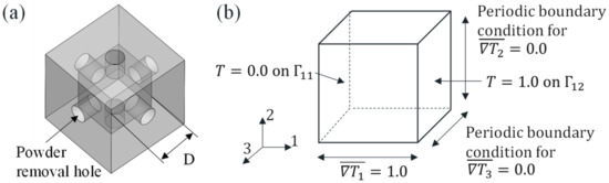
Figure 1.
(a) Base shape of the unit lattice; pore size is considered as the design variable. (b) Boundary conditions of the lattice unit cell for calculating effective thermal conductivity. A unit temperature gradient of is assigned in the i-direction as the Dirichlet boundary condition, and is assigned as the periodic boundary condition.
Moreover, for the unit cell density distribution optimization in the design area Ω, in addition to the heat input q0 from the heat source, the convection heat transfer between the outer surface of the design area Ω and the surrounding environment and the heat exchange via radiation are considered. Accordingly, the boundary condition at Γh is expressed as follows:
where Tamb is the external reference temperature, h is the convection heat transfer coefficient, ε is the surface emissivity of the design area Ω, σ is the Stefan–Boltzmann constant, and q is the heat flow owing to either convection or radiation at the boundary Γh.
2.2. Computation of Effective Thermal Conductivity of Lattice Unit Cell
The basic shape of the lattice unit cell used in this study is presented in Figure 1. The unit cell has a cubic structure, with a cubic internal pore for thermal conductivity control. The effective thermal conductivity tensor, λ*, for this unit cell is obtained by the representative volume element (RVE) method [22,23]. That is, Equation (3), which indicates that the sum of the macroscopic energies of the cell is equal to the sum of local energies, is solved.
where is the temperature gradient for the entire unit cell, and is the local temperature gradient. can be derived using Equation (3) with the boundary conditions of and . ; can be derived in a similar manner. In this study, to assign the temperature gradient as the boundary condition, T = 1.0 was set on one side, whereas T = 0.0 was set on the opposite side; this was to ensure that holds for the boundary between the two sides. was set as the periodic boundary condition.
Moreover, the length D of one side of the cubic pore inside the cell was formulated such that it corresponded with the design variable d . It is worth noting that the effect of thermal radiation was neglected to simplify the problem; this is a common approach in the topology optimization for thermal conduction problems [24].
3. Optimization Procedure
3.1. Problem Statement of Lattice Density Distribution Optimization
Variable lattice density optimization is performed using the unit cell defined in Section 2.2. In this method, an algorithm equivalent to the topology optimization is used [19,20]. In the lattice density distribution optimization, the design area Ω is subdivided into unit lattices. The normalized representative size d of each lattice is regarded as the design variable. In this study, the objective function is the variance of the temperature distribution on the target surface, as expressed in Equation (4). The purpose of this objective function is to unify the temperature distribution. As we predict that the optimal solution is not a fully dense structure, no volume constraint is introduced.
Subject to
Equations (1) and (2)
3.2. Optimization Flowchart
Figure 2 shows the optimization flowchart used in this study. First, for the basic shape of the lattice unit cell, the effective thermal conductivity is calculated using the finite element method. Furthermore, the approximation function of the effective thermal conductivity with respect to the design variable d is constructed. In the optimization iteration, the effective thermal conductivity of each lattice is derived using this approximation equation. The state equation for the design area Ω is then solved using the FEM. The objective function and its sensitivity are calculated based on the FEM results. The density function is then updated using the method of moving asymptotes (MMA) [25]. The parameters of the MMA are the standard ones used for unconstrained problems. Optimization iteration is repeated until convergence. In this research, a fixed number of iterations is introduced as a stopping criterion for the optimization.
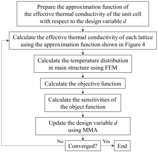
Figure 2.
Flowchart of optimization procedure.
4. Numerical Example of Unit Cell
First, the validity of the proposed method was evaluated by estimating the correlation between the design variable and the effective thermal conductivity for the unit cell defined in Section 2 and Section 3. The unit cell was designed according to the structure described in Section 2.1; the outer length of one side of the cell was set to 5.0 mm. The length of one side of the internal pore D was regulated to correspond with the design variable d by using the equation . The effective thermal conductivity was calculated by varying the design variable in steps of 0.1. The length of one side of the cubic pore was set to the allowable upper limit in order to sustain the minimum wall thickness necessary for the fabrication using metal AM equipment. Moreover, metal-selective laser melting AM equipment was used to fabricate the evaluation test piece used in this study. However, in this method, for the lattice structure fabrication, it is necessary to remove the unmelted powder from the structure after fabrication because the metal powder is selectively melted by a laser. Accordingly, in the design of the unit cell, holes were incorporated to remove the unmelted powder, and the control range of the effective thermal conductivity was evaluated for two cases of the hole diameter: 1.0 mm and 2.0 mm as shown in Figure 3. The material considered was SUS316-L, with a thermal conductivity of . The commercial software COMSOL Multiphysics (COMSOL AB Inc., Stockholm, Sweden) was used for the finite element method (FEM) in this study.
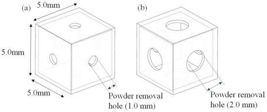
Figure 3.
Basic shape of the unit lattices. (a) Powder removal hole = 1.0 mm. (b) Powder removal hole = 2.0 mm.
Figure 4 shows the correlation between the design variable and the effective thermal conductivity under each condition. For the powder removal hole diameter of 1.0 mm, the thermal conductivity could be regulated within the range of with respect to the design variable in the range of . By contrast, for the powder removal hole diameter of 2.0 mm, the thermal conductivity could be regulated within the range of with respect to the design variable in the range of . In both these cases, the effective thermal conductivity became constant with respect to the design variable beyond the point where the internal pores were smaller than the powder removal hole diameter. The differences in the range of the thermal conductivity control for the same design variable are attributed to the effect of the differences in the volume reduction of the metallic part owing to the size of the powder removal hole. Accordingly, to determine whether the effective thermal conductivity can be calculated using the volume fraction when the bulk state of the unit cell is set to 1.0, the correlation between the volume fraction of the metallic part of the unit cell and the effective thermal conductivity was ascertained for each powder removal hole diameter (Figure 5). Consequently, based on the approximation curve under each condition, it was confirmed that, even under the same volume fraction, changes in the powder removal hole diameter alter the effective thermal conductivity. This is likely because the thermal resistance increases when the powder removal hole diameter is large, even for the same volume, owing to the decrease in the cross-sectional area around the pore. According to these results, it was deduced that, when calculating the thermal conductivity of the unit cell, it is valid to set the design variables considering topology, instead of using the unit cell volume fraction alone.
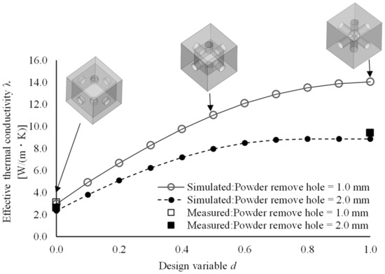
Figure 4.
Simulated and measured results of the effective thermal conductivity with respect to the design variable. Approximation of simulated result for powder removal hole of 1.0 mm: λ = −2.440d3 − 6.376d2 + 19.860d + 2.976, R2 = 1.000. Approximation of simulated result for powder removal hole of 2.0 mm: λ = −1.040d3 − 10.097d2 + 16.404d + 2.300, R2 = 0.999.
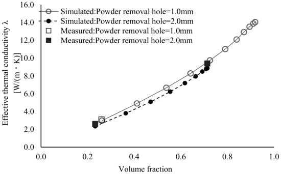
Figure 5.
Simulated and measured results of the effective thermal conductivity with respect to volume fraction. Approximation of simulated result for powder removal hole of 1.0 mm: λ = −13.007d3 − 12.978d2 +17.201d − 0.872, R2 = 0.999. Approximation of simulated result for powder removal hole of 2.0 mm: λ = −13.012d3 − 10.208d2 +13.720d − 0.463, R2 = 1.000.
5. Unit Cell Performance Evaluation
To evaluate the validity of the simulation results for the unit cell described in Section 4, a test piece consisting of unit cells was fabricated using metal-selective laser melting AM equipment, and its thermal conductivity was measured. The difference between the measurements and simulation results was then evaluated. The temperature gradient method was used for measuring the thermal conductivity. As shown in Figure 6a, in the temperature gradient method, one side of the test piece was heated, whereas the other side was cooled; this was to ensure a steady temperature gradient in the thickness direction of the test piece. Thermal conductivity was calculated based on the amount of heat transferred and the temperature difference. This measurement method is a steady-state method; it is considered suitable for a unit cell with an internal pore because it can be applied for the thermal conductivity measurements of materials, such as multilayer materials and composites. Considering the constraints of the measurement method, the dimensions of the test piece composed of the unit lattice were set as 40 mm × 40 mm × 10 mm, as shown in Figure 6b. Three test pieces with different shapes composed of unit cells, as shown in Figure 7, were prepared. For each test piece, the effect of the powder removal hole diameter and the range of the thermal conductivity control for the powder removal hole diameter of 2.0 mm were evaluated. As in the numerical simulation example discussed in the previous section, SUS316-L was used as the test material.
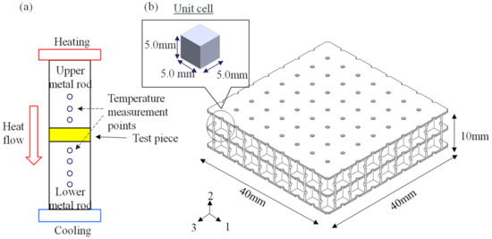
Figure 6.
Outline of experimental equipment for effective thermal conductivity measurements. (a) Schematic of measurement device. One side of the sample was heated and the other side was cooled; a steady temperature gradient was ensured in the thickness direction of the sample. Thermal conductivity was calculated based on the amount of heat transferred and temperature difference. (b) Schematic of test piece comprising the 5.0 mm × 5.0 mm unit cells.
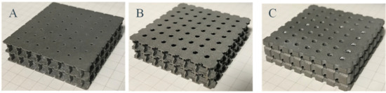
Figure 7.
Images of test pieces for effective thermal conductivity measurements. Labels (A–C) indicate the sample namescorresponding to Table 2.
The results of the evaluation of the test pieces are listed in Table 2. First, it was noted that the fabricated test pieces were 2–10% heavier than their design values. A close examination of the surface and the powder removal holes in the structures revealed that minute amounts of powder remained inside the pores, and some of the powder removal holes had distorted shapes; this may have contributed to the increase in weight. Additionally, it was observed that the measured values of thermal conductivity were approximately 3–11.1% higher than the corresponding simulation results. Considering that the thermal conductivity increased with the volume fraction, as indicated by the simulation results in Section 4, it is likely that the increase in the weight of the fabricated test pieces contributed toward an increase in the measured values of thermal conductivity. Additionally, as shown in Figure 4 and Figure 5, the results indicate that, for both the simulation and the measured values, it is possible to compare the relative superiority of the thermal conductivity over the volume fraction. This demonstrates the validity of the results in Section 4. It was, thus, inferred that it is feasible to use the proposed method for optimization.
Table 2.
Summary of measured and simulated effective thermal conductivities of the lattice unit cells.
6. Numerical Example of Optimized Structure
Using the unit cell designed in Section 4 and Section 5, for the structure shown in Figure 8, an optimized structure to minimize the surface temperature distribution on the target plane was computed. The analytical model is a 1/4 symmetric model for a structure with an internal heat source, and the top surface of the structure was selected as the target plane. Similar to the unit cell, the material assumed was SUS316-L, with a thermal conductivity of . Moreover, given that there are many devices capable of controlling the reference temperature at a specific location in industrial applications (such as molds), for the thermal conduction problem, in addition to the reference and optimized structures, the temperature distribution was evaluated under a condition where the maximum temperature on the target plane was 403.2 K (130 °C). To realize this maximum temperature on the target plane, the heat input from the heat source inside the structure was set in as 5.8–6.2 W/cm2. The heat source was positioned below the mid-point of the structure because there are often constraints on the heat source position depending on the design constraints in practical operations. It was presumed that such constraints may induce non-uniformity in the surface temperature. Moreover, assuming that the structure will be exposed to a room-temperature environment under natural convection conditions, h = 10 W/m2 and T = 293.2 K were set as the parameters for the convection heat transfer between the outer layer of the structure and its surrounding environment. Additionally, assuming heat radiation to the surrounding environment, the emissivity of the structure was set to ε = 0.94 with T = 293.2 K. The emissivity value for the structure was set assuming that black body paint will be applied to the structure in order to eliminate the effect of the texture and oxidation level of the surface during the actual measurements. The bottom surface of the structure was assumed to be insulated. Moreover, a shell with a thickness of 2 mm from the outer skin of the structure was excluded from the design area. The design area consisted of a unit cell with an outer length of 5 mm on one side and a powder removal hole with a diameter of 2 mm, as designed in Section 4 and Section 5. The thermal conductivity of the cell was estimated using the approximate formula for correlation between the design variable and the effective thermal conductivity. For the structure optimization, the initial value of the density function was set to ρ0 = 0.5. The unit cell with a powder removal hole diameter of 2.0 mm was selected to simplify the removal of the remaining powder inside the pore and facilitate the fabrication of larger components. This was based on the weight measurements of the test piece fabricated using the metal AM, as discussed in Section 5, which revealed that the actual weights often exceeded the design values. In the approximated model used in the optimization, the lattice domain is discretized by square elements which has the same size with the lattice, while the shell and heat source domains are discretized by tetrahedron elements. They are formulated as quadratic elements. The total degrees of freedom is 22888.
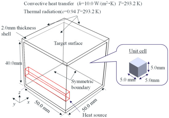
Figure 8.
Analysis domain of the 3D numerical example. The analysis domain was divided into a lattice with 5.0 mm spacing. In the heat conduction problem, the heat source was set inside the analysis domain, and convective heat transfer and thermal radiation were assumed for the outer layer of the structure. A shell with a thickness of 2.0 mm from the outer layer was excluded from the design area.
As shown in Figure 9, with regard to the convergence history of the objective function during optimization, the convergence is quite smooth, and convergence was realized within 30 iterations. Figure 10 shows the detailed geometry of the optimal lattice. After optimizing the thermal conductivity distribution, the thermal conductivity was lowered in the areas closer to the heat source; however, the thermal conductivity increased in regions farther from the heat source. This indicates an improvement in the uniformity of the surface temperature distribution. Figure 11 shows the temperature distributions of the optimal lattice and the reference structures. Table 3 lists the calculation results for thermal conductivity and the temperature distributions in the target plane, for both the reference and optimized structures. As a reference for comparison with the optimized structure, the temperature distribution in the target plane of the structure, the design area of which was composed of the bulk material, was also calculated. For the reference, as the thermal conductivity distribution in the design area was constant under the reference condition, the temperature was higher at the target plane closer to the heat source; by contrast, the temperature was lower at the target plane closer to the heat dissipation side, which was farther from the heat source. Specifically, the temperature difference on the target plane for the reference was 9.7 K, whereas the temperature difference after optimization was 7.1 K, demonstrating an improvement of approximately 30%.
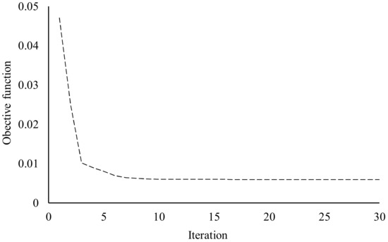
Figure 9.
Convergence history of the objective function for the 3D example.
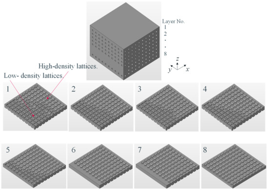
Figure 10.
Detailed geometry of the optimal lattice structure. Labels 1–8 indicate the layer numbers.
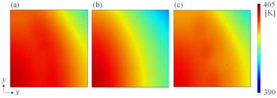
Figure 11.
Temperature distribution on the target surface: (a) optimal lattice using the effective thermal conductivity; (b) reference structure composed of bulk material; and (c) optimal lattice with full-scale geometry.
Table 3.
Summary of the temperature simulation for the optimal lattice structure.
Next, FEM was performed using the full-scale detailed model under the same boundary conditions as in the aforementioned optimization calculations, in order to verify the validity of the modeling with the effective thermal conductivity. In the full-scale detailed model, the whole domain is discretized by the second order tetrahedron elements. The total degree of freedom is 3343914. The results shown in Figure 11c indicate a temperature difference of 7.3 K in the simulation using the 3D model; this is nearly equal to the temperature difference of 7.1 K for the target surface obtained from the optimization calculations as shown in Table 3. The abovementioned results demonstrated the validity of the optimization method using the approximate formula for the effective thermal conductivity of the unit cell evaluated in this study, as well as the 3D modeling procedure utilizing the results of the optimization.
7. Performance Evaluation for Optimized Structure
7.1. Experimental Conditions
The optimal structure derived in Section 6 is experimentally validated. As the optimization was performed using the 1/4 model considering symmetry, the test piece was constructed by integrating the four optimal structures. The test piece is fabricated using the metal powder bed fusion AM device, ProX DMP 200 (3D Systems, Inc., Wilsonville, OR, USA). The material used is 316 L stainless steel.
Figure 12 shows the schematic of the experimental setting for the temperature distribution measurements. The heat source was a cartridge heater with specifications of φ 8.0 mm and 250.0 W; this was inserted inside the structure. The structure was heated such that the maximum temperature on the target surface was approximately 130 °C (403 K), as in the numerical analyses. Moreover, to reproduce the same thermal environment as the boundary condition used in the analysis, a 25 mm-thick insulation board was placed below the structure. The experiments were conducted in a room environment with a stable temperature of approximately 20 °C, without any forced convection. The effects of the surface texture and color were eliminated as far as possible by spray painting the structure using black paint with emissivity ε = 0.94. For the evaluation, two test pieces (samples) were prepared; one was the aforementioned optimized structure fabricated using AM, and the other was the reference bulk structure composed of 316L stainless steel. The temperature measurements were conducted using a thermoviewer and a thermocouple under the steady state after 1.5 h of heating. The thermocouples were placed at the corner and the center of the target surface comprising the minimum and maximum temperatures in the FEM.
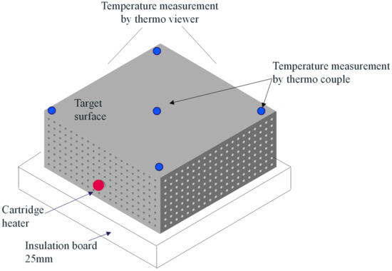
Figure 12.
Schematic of experimental setting for measuring the temperature distribution on the target surface.
7.2. Experimental Results
Figure 13 shows the external shapes for the original model data and the fabricated object. As can be seen, the outline was fully realized. Figure 14 shows the X-ray images of the internal lattice structures corresponding to a design variable value of approximately 0.7. By comparing the X-ray image and the original model data, the error in the geometric size was found to be approximately 0.1–0.2 mm in most areas. Considering the entire test piece (100 mm) and the unit lattice size (5 mm), such an error is sufficiently small. The density of the fabricated object was also measured based on the X-ray image by capturing the total volume of the small cavities. A nearly perfect density of 99.6% was noted. These evaluations indicate that the fabrication quality of the test piece is sufficient for the experiments.
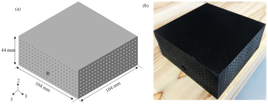
Figure 13.
Test piece for the demonstration experiment: (a) schematic of optimized 3D model, and (b) image of test piece fabricated via metal additive manufacturing. The picture model was painted by black body spray.
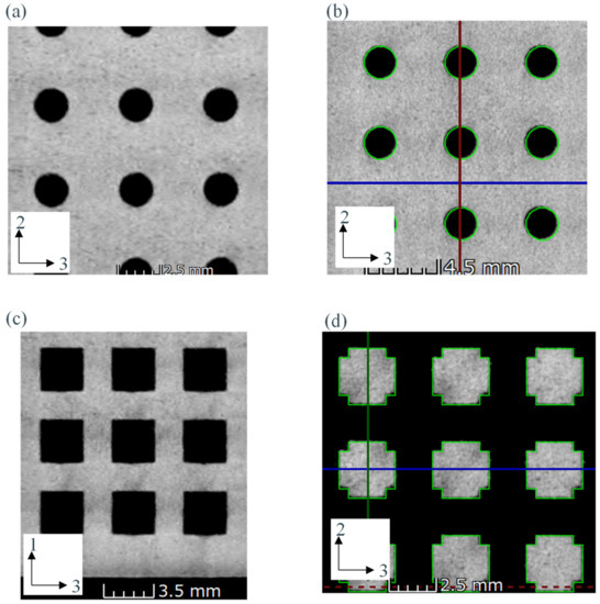
Figure 14.
X-ray images of fabricated model: (a) cross-section of powder removal hole; (b) comparison of hole diameters between fabricated model and 3D model (green line); (c) cross-section of inner pore in the unit cell; and (d) comparison of unit cell structures between the fabricated model and 3D model (green line).
The standard deviation of the temperature distribution on the target surface was evaluated using the thermoviewer. For precise measurements of the temperature, thermocouples were also introduced.
Table 4 lists the results of the temperature measurements, and Figure 15 shows the thermoviewer images for the entire target surface. Both these confirmed that the high-temperature area was larger for the optimized structure than for the reference structure. Moreover, the standard deviation in the target surface temperature was 2.3 K after optimization, as opposed to the deviation of 3.2 K prior to optimization; this represents an improvement of 28%. The maximum and minimum temperatures on the target surface, as measured by the thermocouples, were also improved by 32%. In other words, it was 6.9 K after optimization and 10.2 K before optimization. These values are nearly identical to the analysis results described in Section 6.
Table 4.
Measured results of temperature distribution for reference and optimized structures.
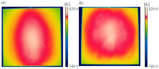
Figure 15.
Measured results of temperature distribution for the reference and optimized structures, as obtained using thermoviewer. (a) Reference structure. (b) Optimal structure.
8. Conclusions
In this study, we expanded the variable lattice density distribution optimization to the minimization of the temperature variations on the target surface. The highlights of this research are as follows:
- The steady-state heat conduction problem is formulated using the effective thermal conductivity of the lattice via the FEM.
- The lattice unit cell is structured as a cube with a cubic void. The effective thermal conductivity of the lattice is derived using the RVE method, and it is experimentally validated using metal AM.
- Polynomials were used to approximate continuous functions that related the design variable to the effective thermal conductivity. The objective function was the variance in the temperature of the target domain. A variable lattice density optimization algorithm was then constructed based on the sensitivity analysis and the MMA.
- The optimal structure reduced the variance in the temperature of the target surface by approximately 30%; the results were experimentally validated using metal AM. The results also indicated that, after optimization, the thermal conductivity in areas closer to the heat source decreased, resulting in a decrease in the maximum temperature of the hot region. Simultaneously, thermal conductivity increased in the regions farther from the heat source, thus improving the temperature distribution uniformity. The error between the numerical and experimental results for temperature was approximately 10%.
In this study, we only attempted using one base unit lattice shape. It is clear that the results can be affected by the lattice base shape. Furthermore, multi-scale optimization of the variable lattice density and the lattice shape is possible. Thus, future works should focus on evaluating the lattice unit cells. Moreover, as managing thermal deformation is a significant issue in forming dies, optimization considering thermal deformation can also be a potential direction of future research. More information please refer to Appendix A.
Author Contributions
Conceptualization, A.U. and A.T.; methodology, A.U., H.G., A.T. and R.M.; software, A.U., H.G., A.T. and R.M.; validation, A.U., H.G., A.T., R.M. and M.K.; investigation, A.U., H.G., A.T., R.M. and M.K.; resources, A.U., A.T. and M.K.; data curation, A.U., H.G., and R.M.; writing—original draft preparation, A.U. and A.T.; writing—review and editing, A.U., H.G., A.T., R.M. and M.K.; visualization, A.U. and A.T.; supervision, A.T.; project administration, A.U. and A.T.; funding acquisition, A.U., A.T. and M.K. All authors have read and agreed to the published version of the manuscript.
Funding
This research was funded by the New Energy and Industrial Technology Development Organization (NEDO) Project to support the discovery of young researchers by the public and private sectors.
Institutional Review Board Statement
Not applicable.
Informed Consent Statement
Not applicable.
Data Availability Statement
Not applicable.
Conflicts of Interest
The authors declare no conflict of interest.
Appendix A. Sensitivity Analysis of the Objective Function
The sensitivity analysis of the objective function is explained in detail here. First, the discretized form of the state equation is considered, as follows:
where K is the thermal conductivity matrix, t is the temperature vector, q is the heat flux vector, and d is the design variable vector. Assuming the scalar objective function f(d), the Lagrangian can be formulated as
where λ is the adjoint vector. Differentiating with the design variable yields the following expression:
When the second term is zero, the sensitivity is obtained as . In this case, the adjoint vector λ must satisfy the adjoint equation . The discrete form of the objective function is , where h is a 0–1 vector specifying the temperatures of the target domain, and i is the vector of ones.
References
- Dambon, O.; Wang, F.; Klocke, F. Efficient mold manufacturing for precision glass molding. J. Vac. Sci. Tech. B 2009, 27, 1445. [Google Scholar] [CrossRef]
- Jeng, M.; Chen, S.; Minh, P.; Chang, J.; Chung, C. Rapid mold temperature control in injection molding by using steam heating. Int. Commun. Heat Mass 2010, 30, 1295–1304. [Google Scholar] [CrossRef]
- Wang, G.; Zhao, G.; Li, H.; Guan, Y. Research of thermal response simulation and mold structure optimization for rapid heat cycle molding processes, respectively, with steam heating and electric heating. Mater. Des. 2010, 31, 382–395. [Google Scholar] [CrossRef]
- Gibson, I.; Rosen, D.; Stucker, B. Additive Manufacturing Technologies; Springer: Berlin/Heidelberg, Germany, 2010. [Google Scholar]
- Kang, J.; Shangguan, H.; Deng, C.; Hu, Y.; Yi, J.; Wang, X.; Zhang, X.; Huang, T. Additive manufacturing-driven mold design for castings. Addit. Manuf. 2018, 22, 472–478. [Google Scholar] [CrossRef]
- Bendsøe, M.P.; Kikuchi, N. Generating optimal topologies in structural design using a homogenization method. Comput. Comput. Method. Appl. M 1988, 71, 197–224. [Google Scholar] [CrossRef]
- Bendsøe, M.P.; Sigmund, O. Topology Optimization: Theory, Methods, and Applications; Springer: Berlin/Heidelberg, Germany, 2003. [Google Scholar]
- Iga, A.; Nishiwaki, S.; Izui, K.; Yoshimura, M. Topology optimization for heat convection problems including design-dependent effects. Trans. Jpn. Soc. Mech. Eng. 2008, 74, 2452–2461. (In Japanese) [Google Scholar] [CrossRef][Green Version]
- Dbouk, T. A review about the engineering design of optimal heat transfer systems using topology optimization. Appl. Eng. 2017, 112, 841–854. [Google Scholar] [CrossRef]
- Costa, G.; Montemurro, M.; Pailhes, J. A 2D topology optimisation algorithm in NURBS framework with geometric constraints. Int. J. Mech. Mater. Des. 2018, 14, 669–696. [Google Scholar] [CrossRef]
- Costa, G.; Montemurro, M.; Pailhes, J. NURBS hypersurfaces for 3D topology optimisation problems. Mech. Adv. Mater. Struct. 2021, 28, 665–684. [Google Scholar] [CrossRef]
- Costa, G.; Montemurro, M.; Pailhes, J. Minimum length scale control in a NURBS-based SIMP method. Comput. Method Appl. Mech. Eng. 2019, 354, 963–989. [Google Scholar] [CrossRef]
- Costa, G.; Montemurro, M.; Pailhes, J.; Perry, N. Maximum length scale requirement in a topology optimisation method based on NURBS hyper-surfaces. CIRP Ann. Manuf. Technol. 2019, 68, 153–156. [Google Scholar] [CrossRef]
- Montemurro, M.; Refai, K. Topology optimization method based on non-uniform rational basis spline hyper-surfaces for heat conduction problems. Symmetry 2021, 13, 888. [Google Scholar] [CrossRef]
- Meng, L.; Zhang, W.; Quan, D.; Shi, G.; Tang, L.; Hou, Y.; Breitkopf, P.; Zhu, J.; Gao, T. From topology optimization design to additive manufacturing: Today’s success and tomorrow’s roadmap. Arch. Comput. Method Eng. 2020, 27, 805–830. [Google Scholar] [CrossRef]
- Koizumi, Y.; Okazaki, A.; Chiba, A.; Kato, T.; Takezawa, A. Cellular lattices of biomedical Co-Cr-Mo-alloy fabricated by electron beam melting with the aid of shape optimization. Addit. Manuf. 2016, 12, 305–313. [Google Scholar] [CrossRef]
- Takezawa, A.; Koizumi, Y.; Kobashi, M. High-stiffness and strength porous maraging steel via topology optimization and selective laser melting. Addit. Manuf. 2017, 18, 194–202. [Google Scholar] [CrossRef]
- Cheng, L.; Zhang, P.; Biyikli, E.; Bai, J.; Robbins, J.; To, A. Efficient design optimization of variable-density cellular structures for additive manufacturing: Theory and experimental validation. Rapid Prototyp. J. 2017, 23, 660–677. [Google Scholar] [CrossRef]
- Wang, X.; Zhang, P.; Ludwick, S.; Belski, E.; To, A. Natural frequency optimization of 3D printed variable-density honeycomb structure via a homogenization-based approach. Addit. Manuf. 2018, 20, 189–198. [Google Scholar] [CrossRef]
- Takezawa, A.; Zhang, X.; Kato, M.; Kitamura, M. Method to optimize an additively-manufactured functionally-graded lattice structure for effective liquid cooling. Addit. Manuf. 2019, 28, 285–298. [Google Scholar] [CrossRef]
- Takezawa, A.; Zhang, X.; Kato, M.; Kitamura, M. Optimization of an additively manufactured functionally graded lattice structure with liquid cooling considering structural performances. Int. J. Heat Mass Transf. 2019, 143, 118564. [Google Scholar] [CrossRef]
- Hansin, Z. Analysis of composite materials: A survey. J. Appl. Mech. 1983, 50, 481–505. [Google Scholar]
- Hill, R. On constitutive macro-variables for heterogeneous solids at finite strain. Proc. Roy. Soc. A Math. Phys. 1972, 326, 131–147. [Google Scholar]
- Takezawa, A.; Yoon, G.H.; Jeong, S.H.; Kobashi, M.; Kitamura, M. Structural topology optimization with strength and heat conduction constraints. Comput. Method Appl. Mech. 2014, 276, 341–361. [Google Scholar] [CrossRef]
- Svanberg, K. The method of moving asymptotes: A new method for structural optimization. Int. J. Numer. Methods Eng. 1987, 24, 359–373. [Google Scholar] [CrossRef]
Publisher’s Note: MDPI stays neutral with regard to jurisdictional claims in published maps and institutional affiliations. |
© 2021 by the authors. Licensee MDPI, Basel, Switzerland. This article is an open access article distributed under the terms and conditions of the Creative Commons Attribution (CC BY) license (https://creativecommons.org/licenses/by/4.0/).