Abstract
Reinforcement Learning (RL) enables an agent to learn control policies for achieving its long-term goals. One key parameter of RL algorithms is a discount factor that scales down future cost in the state’s current value estimate. This study introduces and analyses a transition-based discount factor in two model-free reinforcement learning algorithms: Q-learning and SARSA, and shows their convergence using the theory of stochastic approximation for finite state and action spaces. This causes an asymmetric discounting, favouring some transitions over others, which allows (1) faster convergence than constant discount factor variant of these algorithms, which is demonstrated by experiments on the Taxi domain and MountainCar environments; (2) provides better control over the RL agents to learn risk-averse or risk-taking policy, as demonstrated in a Cliff Walking experiment.
1. Introduction
RL algorithms train a software agent to determine a policy, which can solve an RL problem in the most efficient way possible. Such a policy is termed an optimal policy. The problem is considered solved when the RL agent achieves its desired goal, which varies as per the problem [1]. An RL agent’s objective is generally to minimize its expected long-term costs (or maximize its expected long-term rewards) of problems that can be categorized as episodic and non-episodic depending upon whether a set of goal states exists. Episodic tasks have at least one winning state, such as games like Atari and Chess. An agent maintaining a power plant’s critical temperature is an example of non-episodic RL problems as there is no fixed goal state [2]. Algorithms solving RL problems have potential applications in various domains like games [3,4], robotics [5,6], wireless networks [7,8], self-driving cars [9,10,11]. Two such examples are shown in Figure 1 and Figure 2.

Figure 1.
RL agents beats human benchmark in Atari Games [25].
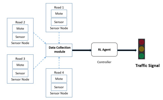
Figure 2.
RL agent as controller for autonomous traffic control system [26].
Many RL algorithms like Q-learning [12], SARSA [13], and Deep Q-learning [14] use a scaling parameter called the discount factor. This parameter exponentially scales down the effect of future costs in the current estimate of the value of a state [15]. This scaling makes the RL algorithms mathematically tractable in case of infinite horizon problems [16]. For the sake of simplicity, in most applications, the discount factor is generally assumed as constant [17]. However, Vincent et al. [18] show that increasing the discount factor, as the training progresses, may result in faster convergence in Atari Games. Later, Edwards et al. [19] show that adjusting the discount factors can be used for reward engineering, which prevents the agent from being stuck in Positive or Negative Reward Hallways (reward loops). These results garner our attention to non-constant discount factors.
One possible way to construct a non-constant discount factor is to take it as a function of iterations itself [20]. Some studies show that a discount factor as a function makes more sense than a constant discount factor in specific settings [21]. For example, incorporating a state-dependent discount factor is a natural setting to model interest rates in financial systems [22]. This use case is based on intuitions from studies on animals. It is common to observe animals show delaying and impulsive behaviour in different tasks [23] which might be because of discounting they use in their brain neurons depending upon the situations [24].
In RL algorithms, contrary to the general belief of choosing a discount factor value close to one, Tutsoy et al. [27] show that the discount factor should be chosen proportional to the inverse of the dominant pole. In other work [28], the author considers the role of the discount factor on both learning and control in a model-free approach. It was suggested by Pitis [20] that the discount factor can exceed one for some transitions if the overall discount is less than one so that the returns are bounded. Hence, the discount factors do not need to be equal for all transitions. Optimality has been studied in Markov Decision Processes (MDP) for unbounded costs using state-dependent discount factor [22] and randomized discount factor [29]. Inspired by Wei [22], Yoshida gave the convergence results of the Q-learning algorithm for the state-dependent discount factor [30]. These studies directly investigate a discount factor’s role for various cases by using both a test problem approach and a general function approximation case. Recently, a state-dependent discount factor model is introduced for infinite horizon case [31]. Other studies utilize state or transition dependent discount factors for better control over the RL agents [31,32,33,34]. This work establishes that the asymmetric discounting of Q-values in a systematic way results in more robust and efficient learning by RL agents. However, breakthrough work in discount factor as a function is done by White [35].
White gave a framework in which the author discussed the use of transition based discounting, that is, a discount factor which is a function of the current state, action, and next state, and proved contraction for generalized Bellman operator [35]. White demonstrated that both non-episodic and episodic tasks could be specified with the help of a transition-based discount. Hence, there is a benefit of using transition-based discount over constant one as the former provides a general unified theory for both episodic and non-episodic tasks. This setting of the discount factor has not been studied yet for Q-learning and SARSA algorithms.
The novelty of our work is the introduction of discount factor as a function of transition variables (current state, action and next state) to the two model-free reinforcement learning algorithms mentioned above and provide convergence results for the same. Experimental results show improvement in the performance of algorithms after using transition dependent discount factor. We have also provided a way to set the discount factor, which can be used in tasks where there are finite state and action spaces, and a positive reward is provided at the goal state. This is fundamentally different from White’s work which proposed to bridge the gap between episodic and non-episodic tasks. In addition, we propose an application of transition dependent discounting to learn risk-averse policies that can prevent frequent high-cost actions by an agent.
Our main contributions are as follows:
- Introduction of transition based discounts in Q-Learning and SARSA algorithms.
- Demonstration of optimal policies in these algorithms with the proposed discount factor setting using stochastic approximation theory to present a generalized result for the convergence of these algorithms.
- Comparison of transition based discount factor with the constant discount factor in Q-learning and SARSA on simulated Taxi domain, MountainCar and cliff-walking environments.
The rest of the paper is organized as follows: Section 2 describes Q-learning and SARSA algorithms. Section 3 introduces the proposed model and Section 4 explains the algorithms and their convergence. Section 5 provides the experimental results against other algorithms. Conclusions are drawn in Section 6.
2. Background
RL algorithms’ objective is to find a mapping for all possible states to actions (also known as policy) that minimizes the agent’s long-term cost in an environment. Reinforcement Learning problems are often modelled as Markov Decision Process (MDP), which is a tuple . Here, S is a set of finite states on which an MDP is defined, is a finite set of all the possible control actions associated with a state . T is the transition probability matrix, is the cost associated with action u in-state i with finite variance and is the discount parameter. We have considered the sets S and U to be finite sets. The algorithms discussed are model-free, that is, the class of algorithms which do not require model (state transition probabilities) of the environment. In both SARSA and Q-learning algorithms, agents generally follow some Greedy in Limit with Infinite Exploration (GLIE) policy (such as -greedy in which each action is taken greedily with probability and randomly otherwise). This policy explores the environment and iteratively calculates its estimate of the Q values for possible state-action pairs.
Q-learning and SARSA try to find an optimum policy , which, if followed, minimizes the total expected cost. This is achieved by defining an action-value function which denotes total expected discounted cost at time t after taking action u in-state i and following policy thereafter. Under the influence of the action value function gives an optimal value which is unique in an MDP and independent of t for a given ().
As we are not looking for any particular optimal policy, we denote as simply . For convenience, we denote as . Let Q-values are stored in a lookup table and all state-action pairs are visited infinitely often.
2.1. Q-Learning
Q-learning algorithm [12] iteratively updates the action-value function or Q-function () which takes state and action as arguments. The algorithm starts with a random table of Q-values for each state-action pair and follows a GLIE policy to choose action. Every action causes a transition from state i to next state u and returns a cost . This cost and the Q-value of the most optimal next state-action pair are used to calculate an estimate. This estimate is then used to update the Q-value of the present state-action pair. The update equation for Q-learning algorithms is given by
Here, is the step size parameter, is a successor state in which the agent arrives after taking action u in-state i. is a scalar constant discount factor. The algorithm draws all the random samples independently. Note that because the estimate is calculated independent of the GLIE policy, it is termed as off-policy. This process is repeated for every state-action pair. The algorithms converge when the change in values are within some threshold. The theoretical convergence result of this algorithm is given in Tsitsiklis et al. [36] and Jaakkola et al. [37].
2.2. SARSA
SARSA, which is State Action Reward State Action for short [38], is an on-policy reinforcement learning algorithm. Here, the estimated return for the state-action pairs is calculated based on the GLIE policy, which the learner is following. This algorithm is very similar to Q-learning except for the way it updates its Q-values. When the agent is in state i, first, it takes action as per the policy it is following (say ) and move to state . Then, the agent selects action v as per the policy and update previous states’ Q-value according to this equation:
This step differentiates SARSA from Q-learning. As in Equation (2), the agent chooses the next state with minimum Q-value, which can be different from the actual next state, whereas, in SARSA, only the next states’ Q-value is considered in the update as in Equation (3). The convergence of this algorithm was given by Singh et al. [39].
3. Transition Dependent Discount Factor
As the name suggests, the parameter discount factor is modelled as function of transition, that is, current state i, action u and next state j. It is denoted by such that ∀, . Hence, different transitions can have different discount factor values. This allows the emphasis of costs from certain transitions and the suppression of others. It can benefit training by avoiding reward loops, much like reward shaping [19]. It is assumed that the values of are stored in a finite length table.
Now with transition dependent discount factor, the update rule for Q-learning is given by:
Similarly, the update equation for SARSA with transition dependent discount is given by:
The Q-learning and SARSA algorithms with the transition dependent discount factor are shown in Algorithms 1 and 2, respectively. Flowcharts of the algorithms are given in Figure 3.
| Algorithm 1 Q-Learning with transition dependent discount |
|
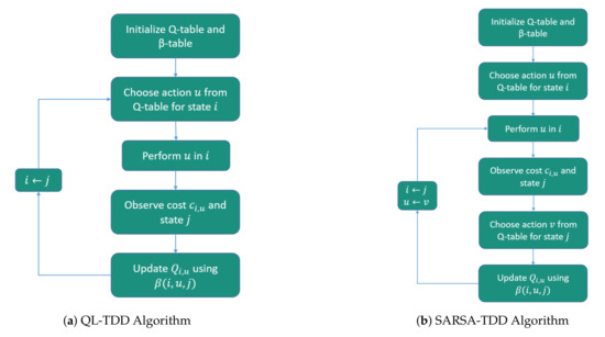
Figure 3.
Flowchart of the proposed algorithms.
Intuition behind Transition Dependent Discount Factor
To understand the intuition of transition dependent discount factor, consider the following finite-state episodic scenario.
Let be the start state and be the terminal state with many states in between them. Let each transition results in a cost of one unit except for transition to terminal state, which results in a cost of unit. Consider the last two transitions in path from to . Let be the set of states which are neighbors of terminal state and be the set of states which are neighbors to the states of set but not with . Thus if an agent goes from state to , the last two visited states are from set and respectively. Note that, the case where last two states are from set does not add value here and does not contradict later arguments. Assume that the states be in set and belongs to set and R is an action required for transition from left to right in Figure 4. Let the discount factor for each transition is , except for those transitions from states in to states in which are caused by the action R. In those transitions, the discount factor value is , where . Then, the Q-value update for the transition from to by action R with transition dependent discount factor is given by:
| Algorithm 2 SARSA with transition dependent discount |
|
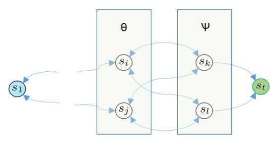
Figure 4.
Simplistic state transition diagram.
Now, for a vanilla Q-learning algorithm, this update would use a constant discount in place of , that is:
Similarly, transitions from to with action R involving and follow similar update rules for transition dependent discounting and and vanilla Q-learning as in Equations (6) and (7). Remaining all other transitions update Q-values using discount factor .
It is clear that as , hence, the Q-value in Equation (6) is less than or equal to the Q-value in Equation (7) (as final cost is negative). Thus, it propagates a lower Q value to previous states in later iterations. Therefore, the updates propagate at a faster rate leading to a shorter learning duration. This argument is valid for all transitions from state set to state set which are due to action R.
Hence, the use of a transition dependent discount factor eventually reduces training time. Similar arguments can be given for SARSA with transition-based discounting.
4. Convergence of Algorithms
Let be the MDP under consideration. Let t be a non-negative integer denoting time. The mapping from state to action is denoted by policy such that where is the set of all policies and action ∀. It is assumed that every action is taken by following some policy. We have defined discount factor as, , satisfying the assumption that ∀. As long as this assumption is satisfied, our analysis shows that discount factor can be any function.
Let be the set of all possible state-action pairs and let N be its cardinality(finite). Let, be the probability space on which are defined as random variables and to be an increasing sequence of - fields which represents the history of algorithm till time t.
On successful completion of both Q-learning and SARSA, the Q values approach for all state-action pairs, and the algorithm is said to converge to optimal. Next, we will present the formal proof for the convergence of these algorithms.
4.1. Q-Learning with Transition-Based Discounts
In Q-learning, instead of using a constant discount factor during Q-values update, a transition-based discount factor is used, which is maintained in a table as mentioned above. With , the update equation of Q-learning (Equation (2)) can be re-written as
Let be the expected cost of a state i which is optimal after action u. We define F to be the mapping from into itself. Its component is given by
After defining everything necessary about Q-learning with the adaptive discount factor, we now present the convergence of this algorithm.
Consider the following result of stochastic approximation equation from Tsitsiklis et al. [36]:
Theorem 1.
Letare random variables defined on the probability spacewhich satisfies this iterative equation:
Then, if following assumptions I, II and III hold, thenwill converge towith probability 1.
Assumption I. Consider the following:
- 1.
- is-measurable;
- 2.
- is-measurable.
- 3.
- is-measurable for every.
- 4.
- We havefor every i and t.
- 5.
- There exist (deterministic) constants A and B ∀such that
Assumption II.
- 1.
- For every i with probability 1,
- 2.
- There exists some (deterministic) constant C such that for every i with probability 1,
Assumption III. There exists a vector, a positive vector v, and a scalar, such that
for some vector v where all elements are equal to 1.
Next, we satisfy all the assumptions of Lemma 1 on Q-learning with a transition based discount factor to prove its convergence.
Proof.
Before we begin, for the sake of simplicity, we assume that v in assumption (III) is a vector of ones. This assumption is valid as we can get it from coordinate scaling of any general positive weight vector. We now discuss each assumption one by one in Q-learning with transition dependent discount factor setting:
Assumption I: This assumption implies that given the past history, it is possible to update at time t. As represents history till time t by definition, hence and are -measurable and -measurable respectively. Thus part (1) and (2) are satisfied. Part (3) follows from the design of Q-learning as it assumes that the requirement of samples is fulfilled by following a simulated trajectory. Updates is dependent on the decision of agent, as it controls which states to visit. Part (4) is inferred from Equation (11) by taking expectations w.r.t. action u on both sides, thus canceling out everything. For Part (5), consider the variance of which is given by:
So if we take variance of Equation (11):
Using Equation (14) and the property of expectations that for some random variable X, we can write the above equation as
It, therefore, satisfies part (5).
Assumption II: This assumption for the step-size parameter is standard for stochastic approximation algorithms. It ensures that all state-action pairs to be visited an infinite number of times.
Let the Q value of this state-action pair be when it is revisited. Then we will have:
4.2. Sarsa with Transition-Based Discounts
The update equation with transition-based discount factor is given by:
To prove the convergence of SARSA with transition-based discounts, we use the convergence result of SARSA [39] under GLIE policy. In GLIE, the probability of choosing a non-greedy action decreases over time, for example, -greedy policy. Other assumptions, like finite states and actions (for lookup table representation) and unlimited visits to all state-action pairs, are similar to Q-learning. Consider the following lemma from Singh et al. [39]:
Lemma 1.
For any random iterative process, , such thataremeasurable, are-measurable andsatisfies:
Thenconverge to zero w.p.1 if the following assumptions hold:
- 1.
- the set X is finite.
- 2.
- w.p.1.
- 3.
- whereandconverge to zero w.p.1.
- 4.
- Varwhere K is some constant.
Hereis an increasing sequence of σ-fields that includes the past of the process.. The notationrefers to some fixed maximum norm.
Proof.
For assumption 1, set X corresponds to the set of state S, which is assumed to be finite; thus, this assumption is satisfied. The second assumption is for the step size parameter for stochastic approximation algorithms and is the same as assumption II of Q-learning. In this lemma, corresponds to as x corresponds to pair of state and action . With this, the stochastic iterative process can be re-written as:
Note that looks similar to the left-hand side of the Equation (17) in assumption III of Q-learning. Both Q-learning and SARSA are very similar algorithms, with the only difference being how the action values are updated in both. Where the update in Q-values of Q-learning follows off-policy, SARSA updates are on-policy. So assumption III of Q-learning is valid here too. Hence,
Thus stating the contraction mapping. Note that differentiates from SARSA with of Q-learning. Now using this information,
This looks similar to the third property of Lemma 1, with the only remaining thing to show is converge to zero with probability 1. Now, as the MDP under consideration is finite, and policy is GLIE, eventually for the state j, action hence . Rest of the arguments relating to the boundedness of are same as Singh et al. [39]. The Q values of the Q-learning algorithm, which updates the same set of state-action pairs, in the same order as SARSA and using min in update equation will bound the Q values of SARSA from below (similarly max will bound from above). Furthermore, due to the similarities with the Q-learning algorithm, Q values of SARSA are also bounded in the same way as the Q values of Q-learning. Similar arguments are there for the boundedness of variance of , thus satisfying lemma’s third and fourth assumptions. □
The convergence proof for SARSA can be concluded by using the following theorem from Singh et al. [39].
Theorem 2.
Consider a finite state-action MDP and fix a GLIE learning policy π. Assume thatis chosen according to π and at time step t, π uses, where thevalues are computed by the SARSA (0) rule. Thenconverge toand the learning policyconverge to an optimal policyprovided that the conditions on the immediate costs, state transitions and learning rates mentioned in Section 2 and Lemma 1 hold and if the following additional conditions are satisfied:
- 1.
- The Q values are stored in a lookup table.
- 2.
- .
Proof.
All the necessary arguments have already been discussed in the lemma 1, hence the proof directly follows from [39]. □
5. Experiments
To demonstrate transition based discounting in Q-learning and SARSA, we performed experiments with a standard taxi domain, mountain car, and cliff walking environment.
Transition dependent discount factor for taxi domain and mountain car environments are constructed in the following way. Every transition to the state, which results in a positive cost, will have slightly more discount factor value than remaining transitions. For these two experiments, we increased the value of those transitions by , and all other transitions have a discount value of . For these values, the algorithms performed optimally. We found algorithms with constant discount performs best when the discount factor’s value is . For another parameter learning rate, the value assigned is . Here, t is the iteration number and is a constant. The value of is chosen heuristically as .
5.1. Taxi Domain
We have considered the Taxi domain environment as given by Dietterich [40]. It is a grid (Figure 5) where the agent (taxi) is allowed to perform six actions, viz. go up, left, right, down, perform pickup, and drops. We have used the original version of this problem, which has four coloured grids, as mentioned in Figure 5. However, the results are comparable even after changing the positions of these coloured grids.
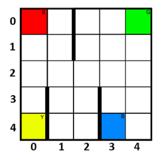
Figure 5.
A 5 × 5 grid of Taxi domain environment.
In this problem, a passenger is waiting in a grid cell to reach a specific destination cell. The goal is to train a taxi agent that can locate a passenger, perform a pickup operation, navigate to the destination cell and perform drop passenger action there in the least amount of time possible. Passenger’s pickup and drop locations are initialized randomly among these coloured blocks when an episode begins. The taxi agent is initialized on any random grid.
Each step results in a cost of 1 unit, successful pickup and drop-off results in a cost of −20 units (or reward of 20). There are three walls within the grid which is marked as bold vertical lines between columns , and . Besides, the boundary cells have walls that prevent the agent from going overboard. Bumping into the walls does not move the agent but induce a penalty of 1 unit (or reward of −1). After initialization, the agent must find the passenger and move towards it using up/down/left/right actions. Then, the agent has to perform a pickup action. A successful pickup costs units, whereas an unsuccessful pickup costs 10 units. The problem is considered solved when the average cost of more than is achieved from 100 consecutive trails.
Table 1 shows the number of episodes it took to solve this problem with vanilla Q-learning, SARSA and Expected SARSA compared with Q-learning with transition dependent discount (QL-TDD) and SARSA with transition dependent discount (SARSA-TDD). Clearly, the proposed algorithms significantly outperforms the baselines by minimum 67 episodes.

Table 1.
Number of episodes it took for Convergence in Taxi domain environment.
5.2. Mountain Car
In this classic control problem, there is a car in a valley controlled by an RL agent, as shown in Figure 6. The goal is to reach the top marked by a flag. The car is not powerful enough; hence, the agent must move it back and forth to build momentum for pushing the car towards its destination. There are only two actions: left and right. Each action costs one unit till the agent reaches the destination. The state-space here is continuous, so it is discretized by bins to apply the finite-state algorithms mentioned in this paper. Figure 7 shows the plot of cumulative rewards obtained versus the number of episodes that favours QL-TDD and SARSA-TDD.
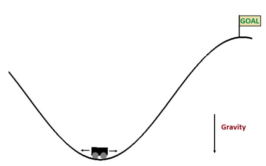
Figure 6.
Mountain Car environment from OpenAi Gym [41].
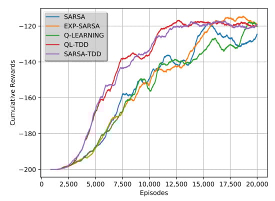
Figure 7.
Expected cumulative rewards for Mountain Car environment.
5.3. Cliff Walking
We can choose transition dependent discount factors to favour certain policy over others. By carefully choosing the discount factor’s value, agents can be made to learn risk-averse or risk-taking policy. This is demonstrated in the Cliff walking environment Figure 8. Here the goal is to reach destination block (G) from the start block (S) while avoiding cliff. Each step results in a cost of 1 unit. However, the cost is 100 if the agent falls from the cliff and the episode terminates. The agent can take one of the four actions in every grid (up, down, left, right). Reaching destination also terminates episode after returning a cost of one unit. Therefore, in order to maximize the expected return, the agent has to reach the destination block in the least number of steps.
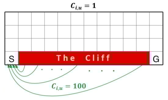
Figure 8.
A 4 × 12 grid of Cliff walking environment. S and G represents source and Goal respectively.
In Q-learning, if all the transitions have same discount () then the learned optimal path obtained is depicted in Figure 9 in orange-coloured arrow. In this path, a single mistake can result in a cost of 100 units. On the other hand, in Q-learning with transition dependent discount factor, the discount factor values for the transitions from left to right in the light blue coloured region is set to . This setting makes the path along with the light blue coloured tiles more favourable due to the increase in Q-values’ value. This new optimal path is depicted in dark blue colour in Figure 9. Note that transitions towards left and down in the light blue coloured cells and all transitions in white coloured cells have a discount value of . The observed results are similar for SARSA with transition dependent discount factor. This new path is safer than the orange coloured path.
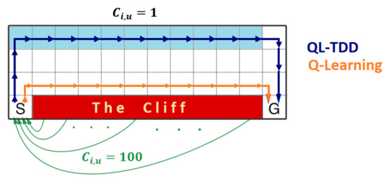
Figure 9.
Light blue tiles are states where discount factor values are changed for transitions towards right.
Thus this experiment demonstrates that by having transition dependent discount values, the agent’s policy can be controlled to behave in either a risk-averse or risk-taking manner.
6. Discussion and Conclusions
The gist of transition dependent discount factor is: we push the signal from goal-states more “intensely” than would otherwise be done and, therefore, be more “goal-oriented”. In this paper, we introduced transition dependent Q-learning and SARSA algorithms. We proved that even by having different discount factor values for all transitions, the algorithms manage to converge to optimal. The experiments demonstrate that by setting the right values of , algorithms can achieve faster convergence. Another benefit of transition dependent discount is more control over the policy learnt. The agent can be encouraged to take risky or non-risky policy by changing the values of as demonstrated in the cliff walking example. Thus, not only it can potentially speed up an RL agent’s learning process, but it can also provide better control over the agent in taking or avoiding risky paths.
In all experiments, the models with a transition dependent discount factor manage to converge to optimal strategy. Finding the correct discount function is a tedious process and a significant challenge that remains. Discount factor as a function also develops a path that leads towards a step in the direction of an adaptive discount factor. This paper concludes that the discount function is a viable choice for discounting, both theoretically and experimentally.
Author Contributions
Conceptualization, A.S., R.G., K.L., and A.G.; methodology, validation, and formal analysis, A.S., K.L. and R.G.; software, A.S. and A.G.; investigation, R.G., K.L. and A.G.; resources, R.G. and A.G.; data curation, K.L. and R.G.; writing-original draft preparation, A.S., K.L. and R.G.; writing—review and editing, A.S., R.G., K.L. and A.G.; visualization, A.S., R.G. and K.L.; supervision, R.G., K.L. and A.G.; project administration, R.G., K.L. and A.G. All authors have read and agreed to the published version of the manuscript.
Funding
This research received no external funding.
Institutional Review Board Statement
Not applicable.
Informed Consent Statement
Not applicable.
Data Availability Statement
Not applicable.
Conflicts of Interest
The authors declare no conflict of interest.
References
- Sutton, R.S.; Barto, A.G. Reinforcement Learning: An Introduction; MIT Press: Cambridge, UK, 1998; Volume 1. [Google Scholar]
- Adams, D.; Oh, D.H.; Kim, D.W.; Lee, C.H.; Oh, M. Deep reinforcement learning optimization framework for a power generation plant considering performance and environmental issues. J. Clean. Prod. 2021, 291, 125915. [Google Scholar] [CrossRef]
- Vinyals, O.; Babuschkin, I.; Czarnecki, W.M.; Mathieu, M.; Dudzik, A.; Chung, J.; Choi, D.H.; Powell, R.; Ewalds, T.; Georgiev, P.; et al. Grandmaster level in StarCraft II using multi-agent reinforcement learning. Nature 2019, 575, 350–354. [Google Scholar] [CrossRef]
- Napolitano, N. Testing match-3 video games with Deep Reinforcement Learning. arXiv 2020, arXiv:2007.01137. [Google Scholar]
- Johannink, T.; Bahl, S.; Nair, A.; Luo, J.; Kumar, A.; Loskyll, M.; Ojea, J.A.; Solowjow, E.; Levine, S. Residual reinforcement learning for robot control. In Proceedings of the 2019 International Conference on Robotics and Automation (ICRA), Montreal, QC, Canada, 20–24 May 2019; pp. 6023–6029. [Google Scholar]
- Lakshmanan, A.K.; Mohan, R.E.; Ramalingam, B.; Le, A.V.; Veerajagadeshwar, P.; Tiwari, K.; Ilyas, M. Complete coverage path planning using reinforcement learning for tetromino based cleaning and maintenance robot. Autom. Constr. 2020, 112, 103078. [Google Scholar] [CrossRef]
- Meng, F.; Chen, P.; Wu, L.; Cheng, J. Power allocation in multi-user cellular networks: Deep reinforcement learning approaches. IEEE Trans. Wirel. Commun. 2020, 19, 6255–6267. [Google Scholar] [CrossRef]
- Leong, A.S.; Ramaswamy, A.; Quevedo, D.E.; Karl, H.; Shi, L. Deep reinforcement learning for wireless sensor scheduling in cyber–physical systems. Automatica 2020, 113, 108759. [Google Scholar] [CrossRef] [Green Version]
- Duan, J.; Li, S.E.; Guan, Y.; Sun, Q.; Cheng, B. Hierarchical reinforcement learning for self-driving decision-making without reliance on labelled driving data. IET Intell. Transp. Syst. 2020, 14, 297–305. [Google Scholar] [CrossRef] [Green Version]
- Kiran, B.R.; Sobh, I.; Talpaert, V.; Mannion, P.; Al Sallab, A.A.; Yogamani, S.; Pérez, P. Deep reinforcement learning for autonomous driving: A survey. IEEE Trans. Intell. Transp. Syst. 2021. [Google Scholar] [CrossRef]
- Hu, B.; Li, J.; Yang, J.; Bai, H.; Li, S.; Sun, Y.; Yang, X. Reinforcement learning approach to design practical adaptive control for a small-scale intelligent vehicle. Symmetry 2019, 11, 1139. [Google Scholar] [CrossRef] [Green Version]
- Watkins, C.J.; Dayan, P. Q-learning. Mach. Learn. 1992, 8, 279–292. [Google Scholar] [CrossRef]
- Rummery, G.A.; Niranjan, M. On-Line Q-Learning Using Connectionist Systems; Department of Engineering, University of Cambridge: Cambridge, UK, 1994; Volume 37. [Google Scholar]
- Bertsekas, D.P. Reinforcement Learning and Optimal Control; Athena Scientific: Belmont, MA, USA, 2019. [Google Scholar]
- Sutton, R.S. Generalization in Reinforcement Learning: Successful Examples Using Sparse Coarse Coding. In Advances in Neural Information Processing Systems; The MIT Press: Cambridge, MA, USA, 1996; pp. 1038–1044. Available online: http://citeseerx.ist.psu.edu/viewdoc/download?doi=10.1.1.51.4764&rep=rep1&type=pdf (accessed on 16 June 2021).
- Kaelbling, L.P.; Littman, M.L.; Moore, A.W. Reinforcement learning: A survey. J. Artif. Intell. Res. 1996, 4, 237–285. [Google Scholar] [CrossRef] [Green Version]
- Arulkumaran, K.; Deisenroth, M.P.; Brundage, M.; Bharath, A.A. Deep reinforcement learning: A brief survey. IEEE Signal Process. Mag. 2017, 34, 26–38. [Google Scholar] [CrossRef] [Green Version]
- François-Lavet, V.; Fonteneau, R.; Ernst, D. How to Discount Deep Reinforcement Learning: Towards New Dynamic Strategies. arXiv 2015, arXiv:1512.02011. [Google Scholar]
- Edwards, A.; Littman, M.L.; Isbell, C.L. Expressing Tasks Robustly via Multiple Discount Factors. 2015. Available online: https://www.semanticscholar.org/paper/Expressing-Tasks-Robustly-via-Multiple-Discount-Edwards-Littman/3b4f5a83ca49d09ce3bf355be8b7e1e956dc27fe (accessed on 16 June 2021).
- Pitis, S. Rethinking the discount factor in reinforcement learning: A decision theoretic approach. Proc. Aaai Conf. Artif. Intell. 2019, 33, 7949–7956. [Google Scholar] [CrossRef] [Green Version]
- Jasso-Fuentes, H.; Menaldi, J.L.; Prieto-Rumeau, T. Discrete-time control with non-constant discount factor. Math. Methods Oper. Res. 2020, 92, 377–399. [Google Scholar] [CrossRef]
- Wei, Q.; Guo, X. Markov decision processes with state-dependent discount factors and unbounded rewards/costs. Oper. Res. Lett. 2011, 39, 369–374. [Google Scholar] [CrossRef]
- Groman, S.M. The Neurobiology of Impulsive Decision-Making and Reinforcement Learning in Nonhuman Animals; Springer: Berlin/Heidelberg, Germany, 2020. [Google Scholar]
- Miyazaki, K.; Miyazaki, K.W.; Doya, K. The role of serotonin in the regulation of patience and impulsivity. Mol. Neurobiol. 2012, 45, 213–224. [Google Scholar] [CrossRef] [Green Version]
- Aydın, A.; Surer, E. Using Generative Adversarial Nets on Atari Games for Feature Extraction in Deep Reinforcement Learning. arXiv 2020, arXiv:2004.02762. [Google Scholar]
- Ning, Z.; Zhang, K.; Wang, X.; Obaidat, M.S.; Guo, L.; Hu, X.; Hu, B.; Guo, Y.; Sadoun, B.; Kwok, R.Y. Joint computing and caching in 5G-envisioned Internet of vehicles: A deep reinforcement learning-based traffic control system. IEEE Trans. Intell. Transp. Syst. 2020. [Google Scholar] [CrossRef]
- Tutsoy, O.; Brown, M. Chaotic dynamics and convergence analysis of temporal difference algorithms with bang-bang control. Optim. Control Appl. Methods 2016, 37, 108–126. [Google Scholar] [CrossRef]
- Tutsoy, O.; Brown, M. Reinforcement learning analysis for a minimum time balance problem. Trans. Inst. Meas. Control 2016, 38, 1186–1200. [Google Scholar] [CrossRef]
- González-Hernández, J.; López-Martínez, R.; Pérez-Hernández, J. Markov control processes with randomized discounted cost. Math. Methods Oper. Res. 2007, 65, 27–44. [Google Scholar] [CrossRef]
- Yoshida, N.; Uchibe, E.; Doya, K. Reinforcement learning with state-dependent discount factor. In Proceedings of the 2013 IEEE Third Joint International Conference on Development and Learning and Epigenetic Robotics (ICDL), Osaka, Japan, 18–22 August 2013; pp. 1–6. [Google Scholar]
- Stachurski, J.; Zhang, J. Dynamic programming with state-dependent discounting. J. Econ. Theory 2021, 192, 105190. [Google Scholar] [CrossRef]
- Zhang, S.; Veeriah, V.; Whiteson, S. Learning retrospective knowledge with reverse reinforcement learning. arXiv 2020, arXiv:2007.06703. [Google Scholar]
- Hasanbeig, M.; Abate, A.; Kroening, D. Cautious reinforcement learning with logical constraints. arXiv 2020, arXiv:2002.12156. [Google Scholar]
- Hasanbeig, M.; Kroening, D.; Abate, A. Deep reinforcement learning with temporal logics. In International Conference on Formal Modeling and Analysis of Timed Systems, Vienna, Austria, 1–3 September 2020; Springer: Berlin/Heidelberg, Germany, 2020; pp. 1–22. [Google Scholar]
- White, M. Unifying Task Specification in Reinforcement Learning. In Proceedings of the 34th International Conference on Machine Learning, ICML 2017, Sydney, NSW, Australia, 6–11 August 2017; pp. 3742–3750. [Google Scholar]
- Tsitsiklis, J.N. Asynchronous stochastic approximation and Q-learning. Mach. Learn. 1994, 16, 185–202. [Google Scholar] [CrossRef] [Green Version]
- Jaakkola, T.; Jordan, M.I.; Singh, S.P. On the convergence of stochastic iterative dynamic programming algorithms. Neural Comput. 1994, 6, 1185–1201. [Google Scholar] [CrossRef] [Green Version]
- Rummery, G.A.; Niranjan, M. On-Line Q-Learning Using Connectionist Systems; Technical Report TR 166; Cambridge University Engineering Department: Cambridge, UK, 1994. [Google Scholar]
- Singh, S.; Jaakkola, T.; Littman, M.L.; Szepesvári, C. Convergence results for single-step on-policy reinforcement-learning algorithms. Mach. Learn. 2000, 38, 287–308. [Google Scholar] [CrossRef] [Green Version]
- Dietterich, T.G. Hierarchical reinforcement learning with the MAXQ value function decomposition. J. Artif. Intell. Res. 2000, 13, 227–303. [Google Scholar] [CrossRef] [Green Version]
- Brockman, G.; Cheung, V.; Pettersson, L.; Schneider, J.; Schulman, J.; Tang, J.; Zaremba, W. Openai gym. arXiv 2016, arXiv:1606.01540. [Google Scholar]
Publisher’s Note: MDPI stays neutral with regard to jurisdictional claims in published maps and institutional affiliations. |
© 2021 by the authors. Licensee MDPI, Basel, Switzerland. This article is an open access article distributed under the terms and conditions of the Creative Commons Attribution (CC BY) license (https://creativecommons.org/licenses/by/4.0/).