Dynamics of Plane Waves in the Fractional Nonlinear Schrödinger Equation with Long-Range Dispersion

Abstract

We analytically and numerically investigate the stability and dynamics of the plane wave solutions of the fractional nonlinear Schrödinger (NLS) equation, where the long-range dispersion is described by the fractional Laplacian ${(-\Delta )}^{\alpha /2}$. The linear stability analysis shows that plane wave solutions in the defocusing NLS are always stable if the power $\alpha \in [1,2]$ but unstable for $\alpha \in (0,1)$. In the focusing case, they can be linearly unstable for any $\alpha \in (0,2]$. We then apply the split-step Fourier spectral (SSFS) method to simulate the nonlinear stage of the plane waves dynamics. In agreement with earlier studies of solitary wave solutions of the fractional focusing NLS, we find that as $\alpha \in (1,2]$ decreases, the solution evolves towards an increasingly localized pulse existing on the background of a “sea” of small-amplitude dispersive waves. Such a highly localized pulse has a broad spectrum, most of whose modes are excited in the nonlinear stage of the pulse evolution and are not predicted by the linear stability analysis. For $\alpha \le 1$, we always find the solution to undergo collapse. We also show, for the first time to our knowledge, that for initial conditions with nonzero group velocities (traveling plane waves), an onset of collapse is delayed compared to that for a standing plane wave initial condition. For defocusing fractional NLS, even though we find traveling plane waves to be linearly unstable for $\alpha <1$, we have never observed collapse. As a by-product of our numerical studies, we derive a stability condition on the time step of the SSFS to guarantee that this method is free from numerical instabilities.

1. Introduction

The fractional Schrödinger equation was first introduced in [1,2] as the path integral of Lévy trajectories. Later, it was also derived from a microscopic lattice system with long-range interactions when passing to the continuum limit [3]. In contrast to its classical counterpart, the fractional Schrödinger equation can model nonlocal interactions, which enables it to describe complex phenomena in various fields; see in [1,2,4,5,6,7,8,9] and references therein. In this paper, we refer to these nonlocal interactions as “long-range dispersion”, because in the classical limit (i.e., for $\alpha =2$ in (1) below), the corresponding term describes group velocity dispersion of linear waves. However, the nonlocality of the fractional Schrödinger equation also introduces considerable challenges in understanding the properties of its solutions [10,11,12,13]. In this paper, we analytically and numerically study the dynamics of the simplest—plane wave—solutions of the fractional nonlinear Schrödinger (NLS) equation and reveal effects of the long-range dispersion on the stability and dynamics of plane wave solutions.

We consider the one-dimensional fractional NLS of the following form [2,3,5,6,11,14]:

$$\begin{array}{c}\hfill i{\partial }_{t}u(x,t)={(-\Delta )}^{\frac{\alpha }{2}}u+\gamma {|u|}^{2}u,x\in \mathbb{R},t>0,\end{array}$$

(1)

where $i=\sqrt{-1}$ is the imaginary unit, and $u(x,t)$ is a complex-valued wave function. The constant $\gamma \in \mathbb{R}$ describes the strength of local (or short-range) nonlinear interactions, where the interactions are repulsive (defocusing) if $\gamma >0$ or attractive (focusing) if $\gamma <0$. The fractional Laplacian ${(-\Delta )}^{\frac{\alpha }{2}}$ is defined via a pseudo-differential operator [5,15,16,17]:

$$\begin{array}{c}\hfill {(-\Delta )}^{\frac{\alpha }{2}}u(x,t):={\mathcal{F}}^{-1}\left[{|\mu |}^{\alpha }\mathcal{F}\left(u\right)\right],for\alpha >0,\end{array}$$

(2)

where $\mathcal{F}$ and ${\mathcal{F}}^{-1}$ denote, respectively, the Fourier transform and its inverse, and $\mu$ is the wave number. In a special case of $\alpha =2$, the definition in (2) reduces to the classical Laplace operator $-\Delta$, and thus Equation (1) becomes the classical (non-fractional) cubic NLS. In this paper, we will focus on the case with $0<\alpha \le 2$, in which case (2) represents the action of a nonlocal operator that describes the long-range dispersion mentioned above [3,10,18,19]. Note that physical relevance of the case $\alpha <1$ has not been universally accepted. Nonetheless, this case was considered for the Majda–McLaughlin–Tabak model [7], and therefore we also include it into the scope of our analysis.

The fractional NLS (1) has two important conserved quantities: the $L^2$–norm, or mass of the wave function,

$$\begin{array}{c}\hfill N\left(t\right):={\int }_{\mathbb{R}}{|u(x,t)|}^{2}dx={\int }_{\mathbb{R}}{|u(x,0)|}^{2}dx=N\left(0\right),t\ge 0,\end{array}$$

(3)

and the total energy,

$$\begin{array}{c}\hfill E\left(t\right):={\int }_{\mathbb{R}}\left[|{\nabla }^{\frac{\alpha }{2}}u{|}^2+\frac{\gamma }{2}{|u|}^4\right]dx=E\left(0\right),t\ge 0,\end{array}$$

(4)

where ${\nabla }^{\alpha }=-{(-\Delta )}^{\frac{\alpha }{2}}$. These conserved quantities can be used as benchmarks to test the performance of numerical methods for the fractional NLS.

Plane wave solutions are the simplest nontrivial solutions of the NLS. Understanding their dynamics and stability provides insight into the behavior of more complicated solutions. In the classical ($\alpha =2$) NLS, stability of the plane wave solutions is well known to critically depend on the sign of nonlinearity: If the nonlinearity is defocusing ($\gamma >0$), the plane waves are always stable, whereas they are subject to long-wave instability in the focusing ($\gamma <0$) case. This instability is known as the Benjamin–Feir instability in the context of water waves or as the modulational instability in the context of plasma physics and nonlinear optics. Unstable perturbations in the classical NLS do not grow without bound. For the fractional NLS, the dynamics of even the simplest nontrivial solution—the plane wave—is still not completely understood. One contribution of this paper is to study stability of both standing and traveling plane waves with respect to small perturbations. To our knowledge, modulational instability of the plane wave solutions of the fractional NLS was studied in [20]; however, its authors considered a different—spatio-temporal, in three dimensions—model, and therefore its results cannot be compared to those presented here.

While linear stability of plane wave solutions can be studied analytically, the nonlinear stage of their dynamics has to be studied numerically. One of the most popular numerical methods in studies of the NLS has been the split-step Fourier spectral (SSFS) method [11,21,22,23,24,25,26,27]. The SSFS method preserves exactly the mass conservation and dispersion relation of the NLS (1). However, the SSFS method could also introduce numerical instabilities which have no analytical counterparts. To interpret its results with confidence, one thus needs to ensure that the method does not introduce numerical, or spurious, instability. Such numerical instability of the SSFS method in simulating the plane wave solutions of the classical NLS has been studied in, e.g., [21,23,24,25,26], but it is missing in the literature on the fractional NLS. A second contribution of this paper is a detailed study of the conditions that ensure numerical stability of the SSFS method when it is used to simulate plane wave solutions of the fractional NLS.

Finally, we study with the SSFS the nonlinear stage of the evolution of perturbed plane waves. Our results for standing plane waves (i.e., those not moving in the reference frame of Equation (1)) are consistent with earlier results by the authors of [14,28], which showed increased localization of the field as $\alpha$ decreased and, in particular, demonstrated wave collapse in finite time for $\alpha =1$. However, to our knowledge, previous studies did not consider dynamics of traveling solutions. (The only exception known to us is in [29]; however, its authors proved the existence of a localized traveling wave solution for $1<\alpha <2$, but did not actually find its analytical or numerical form.) Thus, a third main contribution of this paper is a study of the nonlinear dynamics of traveling (plane) waves, which turns out to be quantitatively (although not qualitatively) different from that of standing waves.

This paper is organized as follows. In Section 2, the stability of plane wave solutions in the fractional NLS is studied by a linear stability analysis. In Section 3, the SSFS method is described, and its numerical stability condition is obtained. In Section 4, we numerically study the dynamics of the unstable plane wave solutions in the fractional NLS, revealing the role played by the long-range dispersion. Conclusions of this study are made in Section 5.

2. Plane Wave Solution and Its Stability

The fractional NLS (1) admits the plane wave solution of the form

$$\begin{array}{c}\hfill u(x,t)=aexp\left(i({\lambda }_{k}x-\omega t)\right),\end{array}$$

(5)

provided that the following nonlinear dispersion relation is satisfied

$$\begin{array}{c}\hfill =|{\lambda }_k{|}^{\alpha }+\gamma {|a|}^2.\end{array}$$

(6)

The constants a and ${\lambda }_k$ are the amplitude and the wave number, respectively, of the plane wave. A wave packet consisting of plane waves (5) with wave numbers in a narrow interval near ${\lambda }_k\ne 0$ would move with a group velocity

$$\begin{array}{c}\hfill v_g=\frac{\partial }{\partial {\lambda }_k}=\alpha \mathrm{sgn}\left({\lambda }_k\right){|{\lambda }_k|}^{\alpha -1},\mathrm{for}{\lambda }_k\ne 0,\end{array}$$

(7)

where $\mathrm{sgn}(·)$ denotes the sign function. For this reason, we will refer to a plane wave with ${\lambda }_k\ne 0$ as a traveling plane wave, contrasting it with a standing plane wave, which has ${\lambda }_k=0$. In simulations reported in subsequent sections, we will consider a finite domain of size L, i.e., $[-L/2,L/2]$, and thus the wave number is chosen as

$$\begin{array}{c}\hfill {\lambda }_k=2k\pi /L,k\in \mathbb{Z}.\end{array}$$

Without loss of generality, we will assume ${\lambda }_k\ge 0$ in this paper.

Due to the nonlinearity of NLS, the plane wave solution (5) is stable only under certain conditions. Here, we will focus on its linear stability analysis in the NLS (1) with the power $\alpha \in (0,2]$. Consider a perturbed solution of the form

$$\begin{array}{c}\hfill \tilde{u}(x,t)=u(x,t)(1+\epsilon (x,t)),\end{array}$$

(8)

where $u(x,t)$ is the plane wave solution in (5), and $\epsilon (x,t)$ is a small perturbation function satisfying $|\epsilon |\ll 1$. We assume that $\epsilon$ is periodic, and it can be expressed in Fourier series as

$$\begin{array}{c}\hfill \epsilon (x,t)=\sum _{l\in \mathbb{Z}}{\widehat{\epsilon }}_l\left(t\right)exp\left(i{\mu }_{l}x\right)\end{array}$$

with ${\mu }_l=2l\pi /L$, for $l\in \mathbb{Z}$. In what follows, we set $\mathrm{Re}\left({\widehat{\epsilon }}_0\left(0\right)\right)=0$ without loss of generality. Indeed, having $\mathrm{Re}\left({\widehat{\epsilon }}_0\left(0\right)\right)\ne 0$ simply rescales the amplitude a of the unperturbed wave (5) in the order $\mathcal{O}\left(\epsilon \right)$.

Substituting (8) into the NLS (1) and taking the leading order terms of $\epsilon$, we obtain

$${\partial }_t\epsilon (x,t)=i\left(|{\lambda }_k{|}^{\alpha }\epsilon -\sum _{l\in \mathbb{Z}}{\widehat{\epsilon }}_l\left(t\right)|{\lambda }_k+{\mu }_l{|}^{\alpha }exp\left(i{\mu }_{l}x\right)-\gamma {|a|}^2({\epsilon }^{*}+\epsilon )\right),$$

(9)

where ${\epsilon }^{*}$ represents the complex conjugate of $\epsilon$. Taking the Fourier transform of (9) and its complex conjugate, we get the following system of ODEs:

$$\frac{d}{dt}\left(\begin{array}{c}{\widehat{\epsilon }}_l\\ {\widehat{\epsilon }}_{-l}^{*}\end{array}\right)=G_l\left(\begin{array}{c}{\widehat{\epsilon }}_l\\ {\widehat{\epsilon }}_{-l}^{*}\end{array}\right),l\in \mathbb{Z}\setminus \left\{0\right\},$$

(10)

where

$$\begin{array}{c}\hfill G_l=i\left(\begin{array}{cc}{\displaystyle |{\lambda }_k{|}^{\alpha }-{\gamma |a|}^2-{|{\lambda }_k+{\mu }_l|}^{\alpha }}& -{\gamma |a|}^2\\ {\displaystyle {\gamma |a|}^2}& -|{\lambda }_k{|}^{\alpha }+{\gamma |a|}^2+{|{\lambda }_k-{\mu }_l|}^{\alpha }\end{array}\right).\end{array}$$

The eigenvalues of matrix $G_l$ are

$$\begin{array}{c}\hfill {\mathsf{\Lambda }}_l^{\pm }=-\frac{i}{2}\left(|{\lambda }_k+{\mu }_l{|}^{\alpha }-{|{\lambda }_k-{\mu }_l|}^{\alpha }\right)\pm \frac{1}{2}\sqrt{{\Delta }_l},\end{array}$$

(11)

where

$${\Delta }_l=-\left[\left(|{\lambda }_k+{\mu }_l{|}^{\alpha }+{|{\lambda }_k-{\mu }_l|}^{\alpha }\right)-2{|{\lambda }_k|}^{\alpha }\right]\left[\left(|{\lambda }_k+{\mu }_l{|}^{\alpha }+{|{\lambda }_k-{\mu }_l|}^{\alpha }\right)-2\left(|{\lambda }_k{|}^{\alpha }-2\gamma {|a|}^2\right)\right].$$

(12)

The solution of system (10) grows exponentially if at least one of the eigenvalues ${\mathsf{\Lambda }}_l^{\pm }$ has positive real part, which occurs if

$$\begin{array}{c}\hfill {\Delta }_l>0.\end{array}$$

(13)

In other words, if the condition (13) holds for at least one $l\in \mathbb{Z}\setminus \left\{0\right\}$, the plane wave solution (5) is unstable.

Below, we will focus on how the instability condition (13) depends on the power $\alpha$ and the wave number ${\lambda }_k$. It is well known that the plane wave solutions in the classical ($\alpha =2)$ NLS are always stable in the defocusing cases and unstable in the focusing cases. Moreover, stability of the plane wave solutions in the classical NLS is independent of its wave number ${\lambda }_k$. In contrast, both these well-established facts no longer hold in the fractional ($0<\alpha <2$) NLS: the plane wave may be unstable in the defocusing case, and its (in)stability is affected by ${\lambda }_k$. These situations are delineated in Theorems 1 and 2 below.

Theorem 1

( Defocusing NLS with $\gamma >0$).

(i) 

For $\alpha \in (0,2]$, a standing plane wave is always stable to infinitesimal perturbations.

(ii) 

For $\alpha \in [1,2]$, a traveling plane wave is always stable, independent of the wave number ${\lambda }_k$.

(iii) 

For $\alpha \in (0,1)$, a traveling plane wave could be unstable if ${\gamma |a|}^2$ is sufficiently large. Moreover, the growth rate of this instability is maximized at modes with $|{\mu }_l|=|{\lambda }_k|$, if the following condition is satisfied:

$$|{\lambda }_k{|}^{\alpha }<\frac{{4\gamma |a|}^2}{2-2^{\alpha }},\alpha \in (0,1).$$

(14)

When $\alpha =2$, our conclusions in Theorem 1 (i)–(ii) reduce to those in the literature [23,25] that a plane wave solution is always stable in the classical defocusing NLS, independent of its wave number. In the fractional NLS, the standing plane wave is always stable, but the stability of traveling plane waves crucially depends on the fractional order $\alpha$.

Figure 1 shows that for $\alpha \in [1,2]$, traveling plane waves are always stable, confirming the conclusion in Theorem 1 (ii). By contrast, they are unstable for $\alpha \in (0,1)$, and the instability is substantially affected by the wave number ${\lambda }_k$. It shows that unstable modes appear in the low-$\mu$ region, and their number generally increases with $|{\lambda }_k|$. If the condition (14) is satisfied, the growth rate of the instability reaches its maximum at ${\mu }_l=\pm {\lambda }_k$ (see Figure 1a,b), confirming the conclusion in Theorem 1 (iii). However, if the condition (14) is not satisfied, there exist stable bands centered at $\pm {\lambda }_k$, which are surrounded by unstable modes (these stable bands are clearly visible in Figure 1d for $\alpha \in (0,0.735)$).

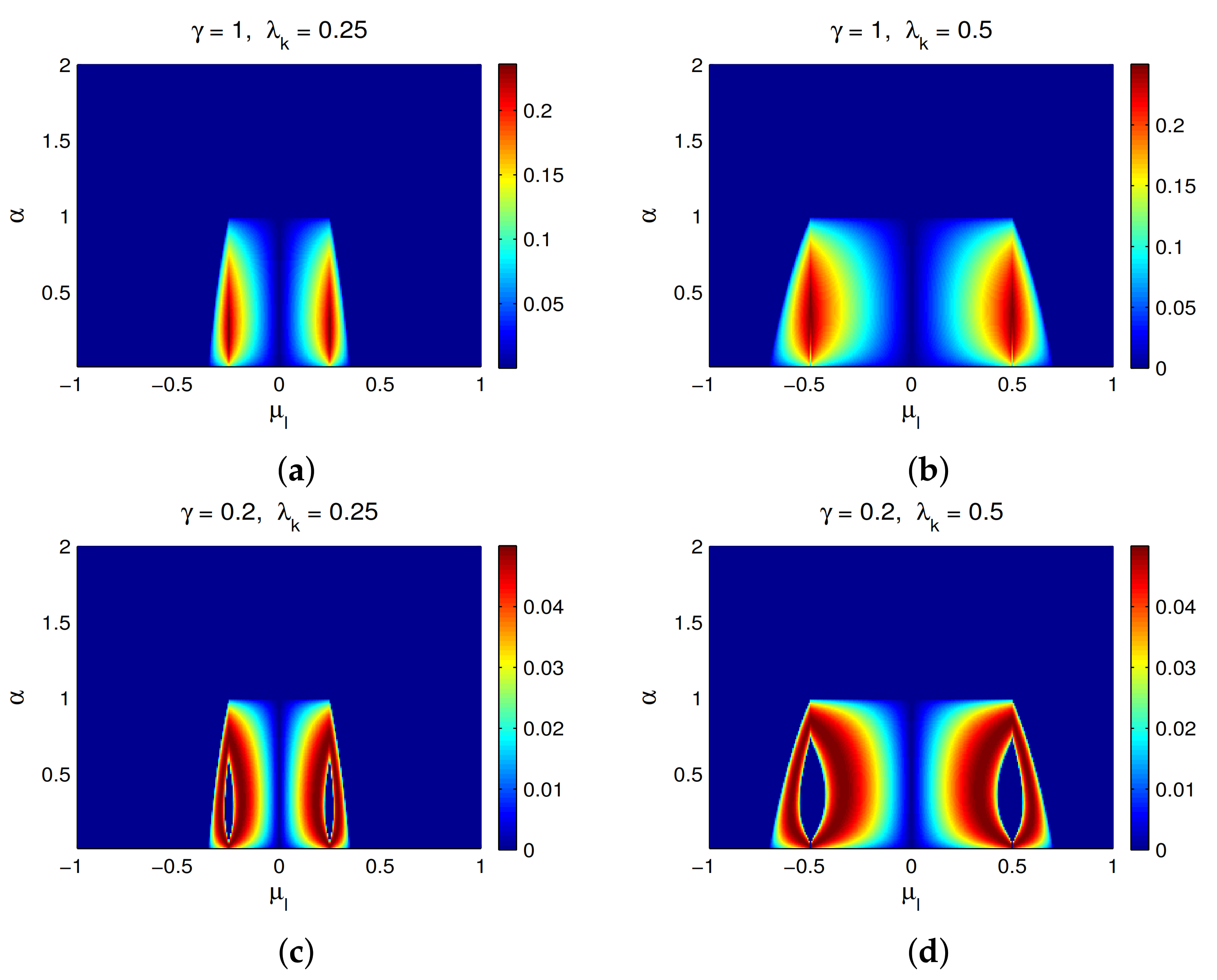
Theorem 2

(Focusing NLS with $\gamma <0$).

(i) 

For $\alpha \in (0,2]$, a standing plane wave is unstable, provided that there is at least one $l\in \mathbb{Z}\setminus \left\{0\right\}$ such that $|{\mu }_l{|}^{\alpha }{<2|\gamma ||a|}^2$. Moreover, the number of unstable pairs is given by

$$n_p=⌊\frac{{L(2|\gamma ||a|}^2{)}^{1/\alpha }}{2\pi }⌋,for\alpha \in (0,2],$$

(15)

where $\lfloor ·\rfloor$ denotes the floor function.

(ii) 

For $\alpha \in (0,2]$, a traveling plane wave is unstable, if L and/or ${|\gamma ||a|}^2$ are sufficiently large.

Theorem 2 (i) implies that if $|{\mu }_1{|}^{\alpha }{>2|\gamma ||a|}^2$, all standing plane waves in the focusing NLS are stable; see the cases of $\alpha \in (0,0.15)$ in Figure 2a.

Otherwise, unstable modes appear in the low-$\mu$ region, i.e., the region of $|{\mu }_l{|<(2|\gamma ||a|}^2{)}^{1/\alpha }$. It implies that for $\alpha \in (0,1)$, the bandwidth of instability is strongly affected by the nonlinearity ${|\gamma ||a|}^2$. In the special case of $\alpha \ll 1$, the bandwidth of instability is exponentially small if ${2|\gamma ||a|}^2<1$ (see Figure 2a), while if ${2|\gamma ||a|}^2>1$, this bandwidth is exponentially large (see Figure 2b, the thin light-green “band” near bottom).

Figure 3a–d presents the stability situation of traveling plane waves in the focusing NLS, which is more complicated than that of standing plane waves. For $\alpha \in (1,2]$, unstable modes always lie in a low-pass band, i.e., instability occurs for small $|{\mu }_l|$. By contrast, two distinctive phenomena are observed for $\alpha \in (0,1]$: (i) there is a “stable gap” in the low-$\mu$ region. Moreover, the bandwidth of this “stable gap” is around $\left(1+{(2-2^{\alpha })}^{1/\alpha }\right)|{\lambda }_k|$ for $\alpha \in (0,1]$, and in the special case of $\alpha =1$ it reduces to ${\lambda }_k$. Indeed, there is ${\Delta }_l<0$ in (12) for the wave numbers satisfying $|{\mu }_l|<{\mu }_{\mathrm{cr}}$, where the critical wave number ${\mu }_{\mathrm{cr}}$ is defined as the positive root of $\left(|{\lambda }_k{+\mu |}^{\alpha }+|{\lambda }_k{-\mu |}^{\alpha }-2{|{\lambda }_k|}^{\alpha }\right)$. Therefore, the wave numbers satisfying $|\mu |\le {\mu }_{\mathrm{cr}}$ are stable. (ii) The bandwidth of instability expands rapidly as $\alpha$ decreases. To show it, we take the Taylor expansion of (12) for $|{\mu }_l|\gg {\lambda }_k$ and obtain

$${\Delta }_l\approx -4\left(|{\mu }_l{|}^{\alpha }-{\lambda }_k^{\alpha }\right)\left(|{\mu }_l{|}^{\alpha }-{\lambda }_k^{\alpha }+2\gamma {|a|}^2\right).$$

(16)

Note that despite condition $|{\mu }_l|\gg {\lambda }_k$, the term of ${\lambda }_k$ cannot be neglected if $\alpha$ is sufficiently small.

In fact, it is this term that is responsible for the expansion of the unstable band compared to the case of ${\lambda }_k=0$. Indeed, the instability condition (13) along with (16) implies the unstable modes:

$$\begin{array}{c}\hfill |{\mu }_l|<{\left({\lambda }_k^{\alpha }+{2|\gamma ||a|}^2\right)}^{1/\alpha }.\end{array}$$

As the exponent $1/\alpha >1$, it suffices for the base to exceed one in order to make $|{\mu }_l|>1$, which makes the right-hand side rapidly increase as $\alpha$ is decreased.

3. Split-Step Fourier Spectral Method

In this section, we first briefly describe the split-step Fourier spectral (SSFS) method for solving the fractional NLS (1) and discuss some of its well-known properties. For our purposes, the first-order SSFS method suffices; if higher accuracy is sought in time, higher-order SSFS method are well known [11,22,27,30,31]. In Section 3.2, we investigate the numerical stability of the SSFS method when it is used to compute plane wave solutions of the NLS.

3.1. Description of the SSFS Method

Let $\tau >0$ be the time step, and define $t_n=n\tau$ for $n=0,1,\dots$ From time $t=t_n$ to $t=t_{n+1}$, one numerically solves the NLS (1) in two steps:

$$\begin{array}{ccc}\hfill & & i{u}_t(x,t)=\gamma {|u|}^{2}u,\hfill \end{array}$$

(17)

$$\begin{array}{ccc}\hfill & & i{u}_t(x,t)={(-\Delta )}^{\frac{\alpha }{2}}u.\hfill \end{array}$$

(18)

For $t\in (t_n,t_{n+1}]$, Equation (17) conserves the quantity $|u(x,t)|\equiv |u(x,t_n)|$, and consequently it reduces to a linear equation for $u(x,t)$. Integrating it in time gives the solution to (17):

$$\begin{array}{c}\hfill u(x,t)=u(x,t_n)e^{-i\gamma |u(x,t_n){|}^2(t-t_n)},t\in [t_n,t_{n+1}].\end{array}$$

To obtain a numerical solution of (18), we consider a computational domain $[-L/2,L/2]$ with periodic boundary conditions. Due to the definition of the fractional Laplacian in (2), the Fourier spectral method is the most natural method for spatial discretization of (18). Choose an even integer $J>0$, and define the mesh size $h=L/J$ and spatial grid points $x_j=-L/2+jh$, for $0\le j\le J$. We take

$$\begin{array}{c}\hfill u(x_j,t)=\sum _{m=-J/2}^{J/2-1}{\widehat{u}}_m\left(t\right)e^{i{\mu }_m{x}_j},\end{array}$$

(19)

where the m-th Fourier mode ${\widehat{u}}_m\left(t\right)$ is defined as

$$\begin{array}{c}\hfill {\widehat{u}}_m\left(t\right)=\frac{1}{J}\sum _{j=0}^{J-1}u(x_j,t)e^{-i{\mu }_m{x}_j},-\frac{J}{2}\le m\le \frac{J}{2}-1.\end{array}$$

Substituting (19) into (18), taking the discrete Fourier transform, and integrating the resulting ordinary differential equation for ${\widehat{u}}_m\left(t\right)$, one obtains

$$\begin{array}{c}\hfill {\widehat{u}}_m\left(t\right)={\widehat{u}}_m\left(t_n\right)e^{-i|{\mu }_m{|}^{\alpha }(t-t_n)},t\in [t_n,t_{n+1}],-\frac{J}{2}\le m\le \frac{J}{2}-1.\end{array}$$

(20)

Combining (20) with (19) leads to an approximate solution of (18).

Finally, denoting the numerical approximation of $u(x_j,t_n)$ by $u_j^n$, one obtains the first-order SSFS method as

$$\begin{array}{ccc}\hfill & & u_j^{n+1,-}=u_j^n{e}^{-i\gamma |u_j^n{|}^2\tau },\hfill \end{array}$$

(21)

$$\begin{array}{ccc}\hfill & & u_j^{n+1}=\sum _{m=-J/2}^{J/2-1}{\widehat{u}}_m^{n+1,-}{e}^{-i|{\mu }_m{|}^{\alpha }\tau }{e}^{i{\mu }_m{x}_j},0\le j\le J-1,n=0,1,\dots \hfill \end{array}$$

(22)

The SSFS method (21)–(22) has spectral accuracy in space and first-order accuracy in time; the latter can be easily improved by employing higher-order split-step schemes [11,22,27,30,31]. This method is explicit and thus easy to implement. In addition, it exactly preserves the discrete $L^2$-norm (mass) of the solution, as well as the dispersion relation $=|{\lambda }_k{|}^{\alpha }+\gamma {|a|}^2$ of plane wave solutions of the fractional NLS for any $\alpha \in (0,2]$ [22]. These quantities are also preserved by higher-order SSFS method. Due to all these features, the SSFS is one of the most popular methods for solving the classical NLS; for the same reasons it can be equally effectively applied to the fractional NLS.

3.2. Stability of the SSFS Method

In this subsection, we study numerical stability of the SSFS method (21)–(22) when it is used to simulate plane wave solutions in (5). The stability condition that we will obtain is essential to enable one to simulate the fractional NLS time-efficiently. That is, it allows one to select the time step small enough so as to avoid numerical artifacts, and yet not too small so as to avoid excessively large simulation times. Our approach is substantially different from those used in [24,25], due to the facts that $\alpha \ne 2$ and ${\lambda }_k\ne 0$. Here, we assume

$${\lambda }_k\ll {\mu }_{max},$$

(23)

where ${\mu }_{max}$ is the maximum wave number resolved by the spectral grids. Note that this assumption does not restrict the value of ${\lambda }_k$ to be small, as one can have, e.g., ${\lambda }_k=0.1{\mu }_{max}\gg 1$ for a sufficiently large ${\mu }_{max}$.

At time $t=t_n$, we consider a perturbed plane wave solution:

$$u_j^n={\tilde{u}}_j^n(1+{\epsilon }_j^n),\mathrm{with}{\tilde{u}}_j^n=a{e}^{i({\lambda }_k{x}_j-\omega t_n)},$$

(24)

where ${\epsilon }_j^n$, with $|{\epsilon }_j^n|\ll 1$, is a small periodic perturbation on $[-L/2,L/2]$ and can be expanded as:

$${\epsilon }_j^n=\sum _{l=-J/2-k}^{J/2-1-k}{\widehat{\epsilon }}_l^n{e}^{i{\mu }_l{x}_j},0\le j\le J-1.$$

(25)

In contrast to (19), a different range of indices is used in the summation of (25). This is the main difference in the analysis for nonzero wave number ${\lambda }_k\ne 0$ from the by-now standard analysis for ${\lambda }_k=0$ [25]. In fact, the perturbation term in (24) is ${\tilde{u}}_j^n{\epsilon }_j^n$, which has effective wave number of $({\lambda }_k+{\mu }_l)\equiv {\mu }_{k+l}$ rather than just ${\mu }_l$. To ensure this wave number fits into the range of $[{\mu }_{min},{\mu }_{max}]$, we have to require ${\mu }_l\in [{\mu }_{min}-{\lambda }_k,{\mu }_{max}-{\lambda }_k]$, resulting in asymmetric summation indices in (25). In order to emphasize this difference compared to the symmetric summation indices in Section 3.1, we use a different letter—l in (25) instead of m in (19). This labeling convention of indices will be used in the remainder of this subsection: m and l, respectively, for the Fourier transform of the solution, ${\widehat{u}}_m$, and the multiplicative perturbation, ${\widehat{\epsilon }}_l$.

Setting $n=n+1$ in (24) and taking its discrete Fourier transform, one obtains

$$\begin{array}{c}\hfill {\widehat{u}}_m^{n+1}=a{e}^{-i{t}_{n+1}}\left\{\begin{array}{cc}{\displaystyle 1+{\widehat{\epsilon }}_0^{n+1},}\hfill & m=k,\hfill \\ {\displaystyle {\widehat{\epsilon }}_{m-k}^{n+1},}\hfill & m\ne k,\hfill \end{array}\right.-\frac{J}{2}\le m\le \frac{J}{2}-1.\end{array}$$

(26)

On the other hand, ${\widehat{u}}_m^{n+1}$ can be independently found from the SSFS scheme (21)–(22). To this end, we substitute $u_j^n$ from (24) into (21) and take the leading order terms of ${\epsilon }_j^n$ to obtain

$$u_j^{n+1,-}={\tilde{u}}_j^n{e}^{-{i\gamma |a|}^2\tau }\left(1+{\epsilon }_j^n-i\gamma {|a|}^2\tau ({\epsilon }_j^n+{\left({\epsilon }_j^n\right)}^{*})\right),0\le j\le J-1.$$

(27)

Substituting (27) into (22) and taking its discrete Fourier transform, we obtain

$$\begin{array}{c}\hfill {\widehat{u}}_m^{n+1}=a{e}^{-i(t_n+\gamma |a{|}^2\tau +|{\mu }_m{|}^{\alpha }\tau )}\left\{\begin{array}{cc}{\displaystyle 1+{\widehat{\epsilon }}_0^n,}\hfill & m=k;\hfill \\ {\displaystyle {\widehat{\epsilon }}_{m-k}^n-i\gamma {|a|}^2\tau ({\widehat{\epsilon }}_{m-k}^n+{\left({\widehat{\epsilon }}_{k-m}^n\right)}^{*}),}\hfill & (m-k)\in {𝒮}_{\mathrm{main}};\hfill \\ {\widehat{\epsilon }}_{m-k}^n-i\gamma {|a|}^2\tau ({\widehat{\epsilon }}_{m-k}^n+{\left({\widehat{\epsilon }}_{k-m-J}^n\right)}^{*}),\hfill & (m-k)\in {𝒮}_{\mathrm{aliased}}.\hfill \end{array}\right.\end{array}$$

(28)

For $m=k$, we have used the convention Re$\left({\widehat{\epsilon }}_0^n\right)=0$, adopted in Section 2. Furthermore, we have split the wave number indices $l\equiv (m-k)$ of the perturbation terms ${\widehat{\epsilon }}_{m-k}^n$ into the “main” and “aliased” sets defined as

$$\begin{array}{ccc}& & {𝒮}_{\mathrm{main}}=\left\{l|-(J/2-1-k)\le l\le J/2-1-k\right\},\hfill \end{array}$$

(29)

$$\begin{array}{ccc}& & {𝒮}_{\mathrm{aliased}}=\left\{l|-J/2-k\le l\le -J/2+k\right\}.\hfill \end{array}$$

(30)

To understand this choice, note that when $(m-k)\equiv l$ is within one of these sets, then the indices of both $\widehat{\epsilon }$- and ${\widehat{\epsilon }}^{*}$-terms in each line in (28) are within the same set. For ${𝒮}_{\mathrm{main}}$, this is evident, while for ${𝒮}_{\mathrm{aliased}}$ this follows from the fact that discrete Fourier transform “wraps” (i.e., aliases) indices modulo J when they fall outside the range $[-J/2,J/2-1]$. Note that the aliased region ${𝒮}_{\mathrm{aliased}}$ was considered in the SSFS stability study for the classical NLS in [24], where stability on the background of traveling waves was studied, but did not need to be considered in the SSFS stability study on the background of a standing plane wave [25], because in that case ${𝒮}_{\mathrm{aliased}}$ is an empty set.

Carrying on and comparing (28) with (26) and their complex conjugates, we obtain the following equations:

$$\left(\begin{array}{c}{\displaystyle {\widehat{\epsilon }}_l^{n+1}}\hfill \\ {\displaystyle {\left({\widehat{\epsilon }}_s^{n+1}\right)}^{*}}\hfill \end{array}\right)=A_l\left(\begin{array}{c}{\displaystyle {\widehat{\epsilon }}_l^n}\hfill \\ {\displaystyle {\left({\widehat{\epsilon }}_s^n\right)}^{*}}\hfill \end{array}\right),\mathrm{for}-\frac{J}{2}-k\le l\le \frac{J}{2}-1-k,$$

(31)

where we let $l=m-k$, and denote s as

$$\begin{array}{c}\hfill s=\left\{\begin{array}{cc}-l,\hfill & \mathrm{if}l\in {𝒮}_{\mathrm{main}};\hfill \\ -(l+J),\hfill & \mathrm{if}l\in {𝒮}_{\mathrm{aliased}}.\hfill \end{array}\right.\end{array}$$

The matrix

$$\begin{array}{ccc}\hfill A_l& =& \left(\begin{array}{cc}{\displaystyle {(1-i\gamma |a|}^2\tau )e^{-i(|{\mu }_{k+l}{|}^{\alpha }-|{\lambda }_k{|}^{\alpha })\tau }}\hfill & {\displaystyle -{i\gamma |a|}^2\tau e^{-i(|{\mu }_{k+l}{|}^{\alpha }-|{\lambda }_k{|}^{\alpha })\tau }}\hfill \\ {\displaystyle {i\gamma |a|}^2\tau e^{i(|{\mu }_{k+s}{|}^{\alpha }-|{\lambda }_k{|}^{\alpha })\tau }}\hfill & {\displaystyle {(1+i\gamma |a|}^2\tau )e^{i(|{\mu }_{k+s}{|}^{\alpha }-|{\lambda }_k{|}^{\alpha })\tau }}\hfill \end{array}\right)\hfill \end{array}$$

has eigenvalues

$${\mathsf{\Lambda }}_{l,\pm }=\left(cos{\theta }_l-\gamma {|a|}^2\tau sin{\theta }_l\right)\pm \sqrt{{\left(cos{\theta }_l-\gamma {|a|}^2\tau sin{\theta }_l\right)}^2-1}$$

(32)

with

$${\theta }_l=\frac{\tau }{2}\left(|{\mu }_l+{\lambda }_k{|}^{\alpha }+|{\mu }_s+{\lambda }_k{|}^{\alpha }-2{|{\lambda }_k|}^{\alpha }\right).$$

(33)

The solution of system (31) will exponentially grow if either $|{\mathsf{\Lambda }}_{l,+}|>1$ or $|{\mathsf{\Lambda }}_{l,-}|>1$. From (32), we then deduce the instability condition summarized below.

Lemma 1

( General instability condition). The unstable modes of the SSFS method in simulating a plane wave solution in (5) satisfy

$$\left|cos{\theta }_l-\gamma {|a|}^2\tau sin{\theta }_l\right|>1,$$

(34)

with ${\theta }_l$ being defined in (33).

We remark that Lemma 1 predicts both analytically unstable modes as described in (13) and numerically unstable modes introduced by the SSFS method. In what follows, we assume that the time step $\tau$ is small enough such that

$${|\gamma ||a|}^2\tau \ll 1,$$

(35)

which is necessary to ensure accuracy of the SSFS method. We then divide our discussion of the instability condition (34) into two parts. On one hand, with assumption (35) the condition $\left(cos{\theta }_l-\gamma {|a|}^2\tau sin{\theta }_l\right)>1$ is satisfied only when $|{\theta }_l|\ll 1$, implying that unstable modes in this case occur only in the main spectral region. Furthermore, the Taylor expansion of $\left(cos{\theta }_l-\gamma {|a|}^2\tau sin{\theta }_l\right)>1$ up to terms $\mathcal{O}\left({\tau }^2\right)$ yields

$$\begin{array}{c}\hfill \left(|{\mu }_l+{\lambda }_k{|}^{\alpha }+|{\mu }_l-{\lambda }_k{|}^{\alpha }-2{|{\lambda }_k|}^{\alpha }\right)\left(|{\mu }_l+{\lambda }_k{|}^{\alpha }+|{\mu }_l-{\lambda }_k{|}^{\alpha }-2(|{\lambda }_k{|}^{\alpha }-{2\gamma |a|}^2)\right)<0,\end{array}$$

i.e., the same condition as in (13). Therefore, the condition $\left(cos{\theta }_l-\gamma {|a|}^2\tau sin{\theta }_l\right)>1$ in (34) predicts the analytically (i.e., truly) unstable modes of the plane wave solutions.

On the other hand, the numerical instability condition of the SSFS method is given by

$$\left(cos{\theta }_l-\gamma {|a|}^2\tau sin{\theta }_l\right)<-1,$$

(36)

which occurs when ${\theta }_l\approx \pi +2n\pi$ (for $n\in \mathbb{Z}$). Then, we have the following results:

Theorem 3

(Numerical stability condition). Assume that the wave number ${\lambda }_k\ll {\mu }_{\max }$ and the nonlinearity ${|\gamma ||a|}^2\tau \ll 1$. Then, the SSFS method remains numerically stable, provided that the time step satisfies

$$\tau <\left\{\begin{array}{cc}{\displaystyle \frac{{\pi }^{1-\alpha }{h}^{\alpha }}{max\left\{(1+{(1-2r)}^{\alpha })/2,{(1-r)}^{\alpha }\right\}-r^{\alpha }},}\hfill & ifr=0,orr\ne 0 and \alpha >{\alpha }_{\mathrm{cr}}\left(r\right)\hfill \\ {\displaystyle \frac{{\pi }^{1-\alpha }{h}^{\alpha }}{(1-2^{\alpha -1})r^{\alpha }},}\hfill & ifr\ne 0 and \alpha \le {\alpha }_{\mathrm{cr}}\left(r\right)\hfill \end{array}\right.$$

(37)

where the ratio $r={\lambda }_k/{\mu }_{max}$, and the critical value ${\alpha }_{\mathrm{cr}}\left(r\right)<1$ is defined as satisfying

$$2-2^{\alpha -1}={\left((1-r)/r\right)}^{\alpha };$$

it is plotted in Figure A1b. Note that the condition in the second line of (37), when it applies, sets a smaller stability threshold than that in the first line.

A detailed derivation of this Theorem can be found in Appendix A. The condition (37) implies that the larger the speed of the simulated plane wave, the larger the time threshold of numerical stability. In simulating the standing plane wave solutions, the stability condition for the SSFS method reduces to $\tau <{\pi }^{1-\alpha }{h}^{\alpha }$ for any $\alpha \in (0,2]$.

Corollary 1

(Classical NLS with $\alpha =2$).

(i) 

For the classical NLS ($\alpha =2$), condition (37) reduces to

$$\begin{array}{c}\hfill \tau <\frac{h^2}{\pi {(1-{\lambda }_k/{\mu }_{max})}^2},\end{array}$$

(38)

in agreement with the conclusions in [25] for ${\lambda }_k=0$ and [24] for ${\lambda }_k\ne 0$.

(ii) 

For the practical case of ${\lambda }_k/{\mu }_{max}\equiv r\ll 1$, the first line of condition (37) reduces to

$$\tau <\frac{{\pi }^{1-\alpha }{h}^{\alpha }}{(1-\alpha r)-r^{\alpha }+O\left(r^2\right)}.$$

Remark 1.

The condition (37) suggests that for $\alpha \ll 1$, the stability threshold of time step may become $\mathcal{O}\left(1\right)$. However, such a large time step cannot be used solely from the accuracy perspective. Therefore, in this case a reasonable requirement to impose on the time step is (35).

The analysis of this section can be generalized to higher-order split-step methods. We have numerically verified that the stability condition (37) remains the same for a fourth-order split-step method, although the growth rate of the numerical instability has been observed to be different. This sameness of the stability condition and the difference of the instability growth rates for the SSFS applied to the fractional NLS parallels that for the case of the classical NLS [32].

4. Dynamics of Plane Wave Solutions

Here, we study the dynamics of unstable plane wave solutions by directly simulating the NLS (1) with the first-order SSFS method. In selected cases, we have verified that using a fourth-order SSFS method does not affect the conclusions. Our main goal here is to highlight effects of the fractional, versus classical, Laplacian, on the dynamics of the plane wave solutions beyond the linear stage of the analytical instability development.

The initial condition is chosen as a perturbed plane wave solution of the following form:

$$u(x,0)=a{e}^{i{\lambda }_{k}x}\left(1+{\epsilon }_{0}cos\frac{2\pi x}{L}\right),-\frac{L}{2}\le x\le \frac{L}{2},$$

(39)

where a and ${\epsilon }_0$ are constants, and $|{\epsilon }_0|\ll 1$. Note that the shape of this perturbation has a maximum at the middle of the computational window and minima at its boundaries. Therefore, for the standing plane waves, this perturbation is expected to favor the emergence of a pulse in the middle of the computational domain. Perturbations that have maxima at different locations will favor formation of pulses there. This all pertains to the initial stage of the evolution; at later times, the pulses begin to move due to their interaction with many different Fourier harmonics created from the background noise, which thus generically have different magnitudes. Nonetheless, our simulations show that various initial perturbations of a similar size may do not affect our conclusions about differences between the fractional and classical NLS.

In the following, we choose ${\epsilon }_0={10}^{-5}$ and $a=\frac{1}{2}$ in (39). Unless stated otherwise, we set domain length $L=5\pi$ with number of grid points $J=2^{13}$. In all cases considered, we selected the time step $\tau$ according to condition (37) so as to avoid numerical instability.

4.1. Standing Plane Waves

In the defocusing NLS, the analysis in Theorem 1 (i) shows that the standing plane waves are always stable for any $\alpha \in (0,2]$, and our numerical simulations confirm this. Therefore, below we report results for the standing plane wave in the focusing NLS. We chose ${\lambda }_k=0$ in the initial condition (39) and $\gamma =-1$ in the NLS (1).

For the parameters stated in the preamble for this Section, formula (15) predicts that for any $\alpha \in (0.76,2]$, there exists one pair of unstable modes with $l=\pm 1$ on the spectral grid ${\mu }_l$, and thus the standing plane wave is linearly unstable. Figure 4 presents the time evolution of $|u(x,t)|$ for different $\alpha$. It shows that the solution remains a plane wave for a short time, and then around $t=50$ (which, of course, depends on the parameters chosen in (39)) one hump appears due to the instability. For $\alpha \lesssim 2$, the hump retains its shape only for a short period of time, after which it dissolves into a delocalized state (a plane wave for $\alpha =2$), then reassembles itself again, and this process goes on approximately periodically. As $\alpha$ decreases, the time interval between the hump reappearances decreases, and both it and the amplitude of the re-emerging pulse become more and more irregular. As $\alpha \to 1^{+}$, the solution tends to form a narrow pulse (see Figure 4 bottom row). For $\alpha \in (0.76,1]$, the plane wave was found to collapse. (For $\alpha <0.76$, there are no unstable modes according to (15), and thus the plane wave remains stable. The more analytically unstable modes exist in the computational domain (which can be controlled either by the domain’s length L or by the wave’s amplitude $|a|$), the earlier the collapse occurs. Furthermore, the modulational instability growth rate, found from Equations (11)–(13), has an evident effect on the time of the collapse occurrence.) The above observations about collapse are consistent with findings in [14,28], which also demonstrated collapse for $\alpha <1$, albeit in their case the initial condition was a localized solitary wave. It is also similar to what has been reported about solutions of the Majda–McLaughlin–Tabak model, a model with nonlocality in both dispersion and nonlinearity, which has been proposed to mimic wave turbulence [4,7,8].

Figure 5 displays the time evolution of the spectrum of the solution $u(x,t)$, with the corresponding density dynamics shown in Figure 4.

In the NLS with $\alpha$ equal or close to 2, the spectrum expands (almost) periodically as the unstable modes evolve. The smaller the fractional order $\alpha$, the more frequently the spectrum expands and shrinks, and also the broader the expanded spectrum becomes. When $\alpha$ is sufficiently close to 1, the spectrum expands quickly after the analytical instability is triggered, but does not shrink back (see Figure 5 for $\alpha =1.1$).

Let us note that for a given power $\alpha$, a smaller nonlinearity (i.e., the value of ${|\gamma ||a|}^2$) results in a less broad spectrum of the emerging pulse (cf. Figure 6 for $\gamma =-0.8$). Additionally, the time required for the formation of a narrow pulse increases as the nonlinearity decreases.

The Fourier spectrum shown in Figure 5 illustrates the role of long-range dispersion that is described by the fractional Laplacian ${(-\Delta )}^{\frac{\alpha }{2}}$. Due to an interplay of nonlinearity with long-range dispersion, the instability at low wave numbers triggers creation of new harmonics in the high wave number region. The smaller the fractional power $\alpha$, the stronger the long-range interactions, and thus the stronger this effect. While the linear analysis predicts this instability, it could not predict that the instability would lead to a dramatic spectral expansion. Numerical simulations were required to reveal this nonlinear stage of the instability development. Our observations are consistent with those reported in the literature [19], where a discrete (with finite inter-site spacing) version of the NLS with long-range interactions was studied. As we noted in Section 1, the continuum limit of such a discrete equation leads to the fractional NLS. In fact, it is stated in [19] that reproducing their results within the framework of a continuous fractional NLS was then an open problem; we have addressed this problem here.

To conclude this section, we present, in Figure 7a,b, snapshots of the field and its Fourier spectrum at time instances shortly before the collapse occurs (the last snapshot is taken within 0.1 time unit from the instance when the Fourier spectrum becomes essentially flat).

A feature to note is the cusp in the spectrum at $\mu =0$. This signals a slow decay of the field u with x, which is due to the long-range interactions enabled by the Lévy index $\alpha =0.9$.

4.2. Effects of a Larger Domain

In this section, we focus on the dynamics of standing plane waves in the focusing NLS when the domain length L increases. Here, we use $\gamma =-1$ and $L=10\pi$, instead of $L=5\pi$ used in the previous subsection. By formula (15), more unstable modes appear as the domain size increases. Specifically, in this case we find that there exist three unstable pairs (i.e., $l=\pm 1,\pm 2,\pm 3$) for any $\alpha \in [1.36,2]$. Their interaction with one another can result in an emergence of more than one pulse; this expectation is indeed borne out by our numerical simulations, reported in Figure 8.

The field dynamics in the classical NLS ($\alpha =2$) appears to be regular. This is likely the consequence of this equation’s integrability and the presence of only a small number of unstable modes, as the computational domain is still relatively short. As $\alpha$ decreases, the evolution of the initially emerged “humps” in the field (around $t=100$) becomes more an more chaotic. This may be explained by the fact that in nonintegrable systems, pulse interaction is usually accompanied by energy transfer from a smaller to a larger pulse (see, e.g., in [33]). Eventually, such repeated interactions lead to formation of a single dominant pulse propagating in a “sea” of small-amplitude dispersive waves. Another feature, most evident from the lower panels of Figure 8, is that a spatially symmetric initial condition results in the formation of a moving pulse (i.e., an asymmetric one). This can be explained by the fact that since the linearly unstable modes, which grow initially, arise from a background noise due to the computer round-off error and thus have different amplitudes (i.e., are asymmetric).

For $\alpha \le 1$, as in the case of the shorter domain, the solution eventually collapses as long as linearly unstable modes exist.

4.3. Effects of Nonzero Group Velocity (7) of the Plane Wave

The analysis in Theorem 1 shows that the traveling (${\lambda }_k\ne 0$) plane waves in the defocusing NLS are always stable if the fractional power $\alpha \in [1,2]$, which is confirmed by our numerical simulations. Therefore, we will focus our following study on the traveling plane wave in the focusing NLS with $\alpha \in (0,2]$ or in the defocusing NLS with $\alpha \in (0,1)$.

Figure 9 shows the time evolution of $|u(x,t)|$ for three representative values of $\alpha$ in the focusing NLS when $\alpha >1$, where ${\lambda }_k=2\pi /L$ (i.e., $k=1$) in the initial condition (39). Equation (13) predicts that there is one pair of unstable modes at $l=\pm 1$ for $\alpha =2$ and $1.9$. Correspondingly, the instability develops into a single soliton-like pulse that moves over a nonzero background.

In the classical NLS, the reappearance of plane wave solution is observed, and the frequency of this recurrence is almost the same as that observed in Figure 4 for standing plane waves. Similar to the observations in Figure 4, a small decrease of $\alpha$ from the classical value $\alpha =2$ leads to a more frequent appearance of the pulse out of the quiescent state. While for $\alpha =1.3$, two unstable pairs occur at $l=\pm 1,\pm 2$, and the behavior of the solution becomes more chaotic due to a nonlinear interaction of these modes (initially) and others excited by them (eventually).

Our simulations show that traveling plane waves in the focusing NLS with $\alpha \in (0,1]$ also collapse, but the occurrence of collapse is progressively delayed by the greater values of ${\lambda }_k$ (with all other parameters being fixed).

Table 1. Collapse time $t_{\mathrm{col}}$ of traveling plane waves in the focusing NLS with $\gamma =-1$ and $L=5\pi$, rounded to the nearest 5 units.

$\mathit{\alpha }$	0.9	0.8	0.7	0.6	0.5
$k=1$	125	120	110	105	80
$k=5$	290	255	245	205	85
$k=20$	>500	355	285	240	215

shows the collapse time in the focusing cases, where the collapse time $t_{\mathrm{col}}$ is defined as the instance where the magnitude of the Fourier component at the edge of the computational spectral window reaches ${10}^{-5}$. While this number is, of course, chosen arbitrarily, replacing it with, say, ${10}^{-3}$ or ${10}^{-7}$ would cause only an insignificant change in the numbers reported in Table 1 and would not change the trends observed. This is because, as earlier for the case of the standing plane wave, collapse in the x-space corresponds to the continuing broadening of the solution’s Fourier spectrum. Once this spectrum increases by several orders of magnitude at the edges of the computational spectral window, the solution can no longer be considered valid. Of course, we verified that doubling the width of the computational spectral window would not prevent the solution’s spectrum from continuing to broaden; therefore, doubling that width only insignificantly affected the collapse times.

We find that for a given ${\lambda }_k$, collapse of solution appears earlier for a smaller $\alpha$. This is the opposite of the situation with the standing wave’s collapse and is explained by the magnitude of the modulational instability growth rates in the two cases. Indeed, for the standing wave, this rate decreases with decreasing $\alpha$ (see Figure 2) and disappears for some small enough $\alpha$ (see the discussion in Section 4.1), it retains its value for a traveling wave as $\alpha$ decreases (see Figure 3). On the other hand, for a given $\alpha$, the collapse is delayed by increasing ${\lambda }_k$. We hypothesize that this may occur because for a larger ${\lambda }_k$, unstable modes ${\mu }_l$ appear at larger $|l|$ (see Figure 3); a possible causal link is discussed at the end of next paragraph.

Snapshots of the solution and its spectrum evolving towards collapse are shown in Figure 10a,b.

The last snapshot is taken within 0.2 time unit before the collapse occurs. A few observations follow from this figure. First, similar to Figure 7b, the spectrum has a cusp at the top, indicating some long-range “order” present in the solution, in agreement with the presence of long-range interactions due to the fractional Laplacian with a low value of $\alpha$. Second, the following scenario of collapse can be deduced. The initial small corrugation grows to a finite size and develops a so-called dispersive wave region, seen as faster oscillations on the right side of each of the periods of the sinusoid for $t=156$. Next, due to these faster oscillations moving through the slower corrugation, there form “humps” with slightly different amplitudes ($t=278$). Due to their interaction with one another, one dominant “hump” forms ($t=286$). This is similar to the behavior observed in other non-integrable systems [33], where the dominant pulse “sucks in” the energy from the ambient field and smaller pulses via collisions with them. It is this dominant pulse that subsequently undergoes collapse. Finally, this scenario explains the reason behind the delay of the collapse caused by a nonzero ${\lambda }_k$ of the initial wave. Apparently, collapse requires that a certain “amount” of the field be concentrated near a given location. As long as there is a corrugation with peaks of the (approximate) sinusoid of similar amplitude, collapse cannot form. However, as soon as “enough” energy has been absorbed by the dominant pulse, collapse becomes possible. The larger ${\lambda }_k$, the smaller the period of the corrugation, and thus the smaller the energy within each one of its periods, and the longer it takes for a sufficient amount of energy to amass near a given location to begin the onset of collapse.

Two more remarks are in order. First, we stress that this ability of the smaller period of the initial corrugation to delay the onset of collapse was stated for the condition that $\alpha$ is fixed. Indeed, as one takes $\alpha$ so small that the results of Section 2 (see Figure 2) predict a wide band of modulationally unstable modes (e.g., for $\alpha =0.15$), the corrugation at the initial stage of the evolution is quite irregular (due to many modes growing at a similar rate). Yet, the fact that $\alpha$ is smaller, and hence the dispersion term ${(-\Delta )}^{\alpha /2}$ has a significantly longer range, acts to overcome the effect of this irregularity and promotes collapse; the latter is found to occur significantly earlier than for $\alpha =0.9$.

Second, while the smaller period of the initial corrugation can only delay, but not arrest, collapse, a recent study [34] has shown that a trapping potential can arrest it. This is consistent with the fact that collapse is caused by the interaction of the field over a sufficiently large range, and a suitable trapping potential is able to essentially truncate this range by localizing the field.

To conclude this subsection, we briefly comment on the defocusing NLS with $\alpha \in (0,1)$. In this case, although the traveling plane waves are also unstable, their dynamics are substantially different from those in the focusing case. No collapse of solution is observed, and the evolution of the solution is qualitatively similar to that in the focusing NLS with $\alpha >1$, shown in Figure 9.

5. Conclusions

In this paper, we investigated the stability and dynamics of the plane wave solutions of the fractional NLS from both analytical and numerical perspectives. The comparison between the classical and fractional NLS were made to understand the role of long-range dispersion in the fractional NLS.

First, in Section 2, we showed that modulational stability of the plane wave solutions to small perturbations can be significantly different in the fractional NLS (1) compared to its classical counterpart when the Lévy index $\alpha \in (0,1)$. In the defocusing ($\gamma >0$) NLS, the standing plane wave solution (i.e., ${\lambda }_k=0$) is always stable for any $\alpha \in (0,2]$. In contrast, the traveling plane wave solution (i.e., ${\lambda }_k\ne 0$) is stable only for $\alpha \in [1,2]$. In the focusing ($\gamma <0$) NLS, the plane wave solution can be linearly unstable for any $\alpha$ and ${\lambda }_k$. Furthermore, unstable modes occur at low-frequency region for $\alpha \in [1,2]$, but they appear at relatively high-frequency region for $\alpha \in (0,1)$, which implies that the dynamics of the plane wave solution (before they collapse) for $\alpha \in (0,1)$ could be more chaotic.

Second, in Section 3, we studied stability of the split-step Fourier spectral (SSFS) method in simulating the dynamics of the plane wave solution of the fractional NLS. This is essential in order to guarantee that the numerical solution does not suffer a blow-up due to purely numerical artifacts; then, one can ascertain that, if the solution undergoes collapse, it reflects the true behavior of the analytical solution. We obtained an expression for the time step threshold below which numerical instability does not occur. This threshold depends on both the parameter $\alpha$, of the NLS, and ${\lambda }_k$, of the simulated plane wave. In particular, for smaller $\alpha$, this threshold can be quite large, and then the time step should be chosen to satisfy the requirement of accuracy, rather than stability, of the numerical method.

Third, in Section 4, we studied the nonlinear stage of the plane wave instability by directly simulating the NLS. For the initial condition being a perturbed standing plane wave in the focusing NLS, we found that the perturbation generically develops into a localized pulse on a nonzero background; the lower the Lévy index $\alpha >1$, the more localized the pulse. In the Fourier space this corresponds to of a significant widening of the solution spectrum, which expands well beyond the band of modulationally unstable modes found by the linear stability analysis. For $\alpha >1$, the pulse undergoes “breathing”, whereby it narrows and broadens intermittently. For $\alpha \le 1$, the pulse localization (in x-space) eventually leads to its collapse, in agreement with findings in [14,28].

We also found that the increase of the group velocity of the plane wave (so that the latter is traveling as opposed to standing) in the focusing NLS delays the formation of a localized pulse (or pulses), for a given fractional index $<1\alpha \le 2$, and delays the onset of collapse, for $\alpha <1$. To our knowledge, this has not been reported before. We also presented a hypothesis as to why this delay could occur. In the defocusing case, even though traveling plane waves are found to be linearly unstable for $\alpha <1$, that instability does not not lead to collapse of the solution.