Optimal Trajectory Synthesis for Spacecraft Asteroid Rendezvous

Abstract

Several researchers are considering the plausibility of being able to rapidly launch a mission to an asteroid, which would fly in close proximity of the asteroid to deliver an impulse in a particular direction so as to deflect the asteroid from its current orbit. Planetary motion, in general, and the motion of asteroids, in particular, are subject to planetary influences that are characterised by a kind of natural symmetry, which results in an asteroid orbiting in a stable and periodic or almost periodic orbit exhibiting a number of natural orbital symmetries. Tracking and following an asteroid, in close proximity, is the subject of this paper. In this paper, the problem of synthesizing an optimal trajectory to a NEO such as an asteroid is considered. A particular strategy involving the optimization of a co-planar trajectory segment that permits the satellite to approach and fly alongside the asteroid is chosen. Two different state space representations of the Hill–Clohessy–Wiltshire (HCW) linearized equations of relative motion are used to obtain optimal trajectories for a spacecraft approaching an asteroid. It is shown that by using a state space representation of HCW equations where the secular states are explicitly represented, the optimal trajectories are not only synthesized rapidly but also result in lower magnitudes of control inputs which must be applied continuously over extended periods of time. Thus, the solutions obtained are particularly suitable for low thrust control of the satellites orbit which can be realized by electric thrusters.

1. Introduction

Near-earth objects (NEOs) moving in resonant, Earth-orbit like orbits are potentially important, as there is always the possibility of a few of them colliding with the Earth at some point in the future. One example is 3753 Cruithne, the Earth’s first co-orbital asteroid discovered in 1986. In 1997, 3753 Cruithne was found to move around the Earth in a horseshoe orbit. However, it was found not to follow the same orbit as the Earth around the Sun and so cannot strictly be called a co-orbital asteroid.

The object is 2002 AA29, found to be closely following Earth’s orbit in a reversible horseshoe orbit. It is known to become a temporary second moon to the Earth from time to time, with the next rendezvous expected in 2600. Its orbit is special as it approaches the Earth on one side, as it did in 2003, and then in about 95 years sweeps to the other side of the Earth. Calculations show that in a time frame of 600 years, this asteroid will orbit the Earth, once a year for 50 years. In a sense, its orbit can resemble that of a satellite. Behaviours such as the above, involving large amplitude oscillations of the eccentricities and inclinations, could in principle be predicted by the Kozai–Lidov mechanism, which is a secular phenomenon in the case of co-orbiting bodies and involves a family of resonance type librations and bifurcations of the equilibrium states, leading to set of stable Kozai resonance states. The coupling of large oscillations of eccentricities and inclination with the continuous motion or libration of the argument of the perhelion is known as the Kozai resonance (Kozai [1]).

In the co-orbital region of the Earth, three types of orbit can occur: tadpole, horseshoe and quasi-satellite orbits. Moreover, spatial tadpole or horseshoe orbits could merge with quasi-satellite orbits and transitions between different types of orbits could appear, in principle. Co orbital asteroids (Brasser, [2]) with tadpole orbits are also known as trojans as they librate about the trojan Lagrangian points of the Sun–Earth and third body system. Horseshoe orbits enclose the L4, L3 and L5 points while Tadpole orbits oscillate or librate only about the L4 or L5 Lagrangian points. Horseshoe orbits librate over much larger amplitude and consequently their shape resembles a horseshoe. Quasi satellite orbits are co-orbital orbits with a high eccentricity so part of the orbit lies well beyond the planet’s sphere of influence and could be unstable in the long term.

Another Earth co-orbital asteroid recently discovered is designated 2010 SO16, and is on a “horseshoe” class orbit. Since its discovery eight other asteroids, 2010 TK7, 2013 BS45, 2013 LX28, 2014 OL339, 2015 SO2, 2015 XX169, 2015 YA and 2015 YQ1 have also been added to list of Earth co-orbiting satellites. Over 24 Earth co-orbital asteroids that have been discovered so far, only 2010 TK7 is a trojan asteroid (Connors, Wiegert and Veillet, [3]) and its orbit is a tadpole or trojan orbit (Dvorak, Lhotka and Zhou, [4]). While it is stable in the short term, its stability in the long term over periods ranging from 10,000 to a million years is questionable. In 2016, HO3, an asteroid discovered on 27 April 2016, is possibly the most stable quasi-satellite of Earth. As it orbits the Sun, 2016 HO3 appears to circle around Earth as well. It is too distant to be a true satellite of Earth, but is the best and most stable example of a quasi-satellite, a type of near-Earth object. They appear to orbit a point other than Earth itself, such as the orbital path of the NEO asteroid 3753 Cruithne. Other small natural objects in orbit around the Sun may enter orbit around Earth for a short amount of time, becoming temporary natural satellites. To date, the only confirmed example has been 2006 RH120 in Earth orbit during 2006 and 2007, though further instances are already predicted. The increasingly high number of potentially hazardous asteroids discovered so far has led to the concept of asteroid deflection (Izzo and Rathke [5]). The problem of artificially changing the orbit of an asteroid to avoid possible future impacts is discussed from the orbital mechanics point of view, by Izzo, Olympio and Yam [6] and the consequences of the deflection of an asteroid by Rathke and Izzo [7]. Izzo et al. [8] discussed the computation of optimal trajectories for the impulsive deflection of near Earth objects.

The primary idea is to give the asteroid an impulse in a particular direction so as to deflect the asteroid from its current orbit and place it in a new orbit which is the preferred orbit of the asteroid in order to avoid a possible collisions. Possibilities of collisions are found by evaluating the minimum orbit intersection distance (MOID). Phenomenon such as the Kozai resonance offer protection from possible collision with several of the asteroids (Libert and Tsiganis [9]). However, there are several others and the potential threat of a collision with an asteroid remains (Domingos and Winter [10]). For this reason, several researchers are considering the need and plausibility of being able to launch a mission to an asteroid, which would fly in close proximity to the asteroid and then deliver the impulse in a particular direction so as to deflect the asteroid from its current orbit and place it in another orbit. Based on the currently available methods of trajectory design such a mission could take up to three years, before a satellite could arrive at an asteroid and fly alongside it in order to be able to deliver a precomputed impulse to it. There is also a need to minimize the fuel requirements in such a mission. Thus, methods are being developed so as to reduce the overall fuel requirements to complete such mission within the constraints of currently available technologies.

In order to compare trajectories and times, a baseline reference trajectory is essential. The initial conditions for the baseline trajectory computation were chosen in the following way: for the Trojan asteroid, the almost stationary orbital elements, the semi-major axis, orbit inclination and the argument of the perihelion and the non-stationary orbital elements, the mean anomaly ‘M’, the argument of the ascending node ‘$\mathsf{\Omega }$’ and the eccentricity ‘e’, were defined from values known on a particular Julian day. For the Earth, the corresponding orbital elements were obtained for the same Julian day from JPL’s Horizon’s website. The integrations were started in the ecliptic plane. The satellite was assumed to be at the edge of Earth’s sphere of influence (SOI) and an impulse was given to it so it intersects the asteroid’s orbit plane. At this node, a further impulse is provided to change the satellites inclination and align its orbit plane with that of the asteroid. Now the satellite and the asteroid are on the same plane but moving in slightly different orbits and with different speeds. When the phase angle between the two is relatively small, an optimally calculated continuous thrust is applied to the satellite so it eventually flies alongside the asteroid. The above methodology could be applied to planning a trajectory to any of the asteroids named in this paper.

The calculation of the optimal segment and the associated thrust history applied in the baseline reference trajectory is done using the HCW linearized equations of relative motion. The HCW equations (Clohessy and Wiltshire [11]) assume that both the target body and the chaser satellite are in near locally circular orbits and that the relative perturbations acting on the chaser satellite relative to the target body are small. The HCW equations may be extended to include all the nonlinearities and Earth oblateness perturbations (Kuiack and Ulrich [12], Vepa [13]). The assumptions on which the derivation of the HCW linearized equations of relative motion is based, are quite restrictive and to initiate a change in both the change in the position and velocity of the satellite so it flies alongside or just behind the target body, the application of the continuous thrust should be done when the phase angle between the two is within certain acceptable limits. Of course, there is always the option of using the full nonlinear equations of relative motion of the chaser satellite relative to the target body. An alternate approach is to use the full nonlinear equations of relative motion, with true anomaly as the independent variable. It is expected that such an approach would provide some flexibility in choosing the optimal trajectory over which the continuous thrust is applied to the chaser satellite. It must be mentioned at this stage, extensive computations of optimal relative motion trajectories have been carried out by Patel, Udrea and Nayak [14] and by Frey et al. [15].

In this paper, the problem of synthesizing an optimal trajectory to a NEO such as an asteroid is considered. In particular, the focus is on the synthesis of low, continuous thrust, trajectories that could be realized by the use of electric propulsion. While there are several possible alternate strategies that one could adopt, a particular strategy involving the optimization of a co-planar trajectory segment that permits the satellite to approach and fly alongside the asteroid is chosen. It must be said, that HCW equations are not generally used for orbit prediction. They are used mainly for guidance and control applications. The HCW equations of motion are derived by linearizing about a reference solution, and as such they are valid in the vicinity of the target point. When used far away from the reference point their validity is questionable, and therefore, are not generally used to design trajectories starting from Earth and flying to an asteroid, which requires solving a fully nonlinear optimal control problem. In this application, they have been used when the spacecraft is in close proximity of the asteroid. Initially, the spacecraft is manoeuvred into a position close to the asteroid by a minimal set of discrete impulses. Once the spacecraft is in close proximity to the asteroid, the HCW equations may be used to synthesize a co-planar trajectory segment that permits the satellite to approach and fly alongside the asteroid. How close the spacecraft should be to an asteroid before one can adopt the HCW equations, depends on a number of factors such as the differences in the orbital elements of the Cartesian position coordinates. There are two cases to consider, without and with perturbations. When the perturbation effects on the asteroid and the spacecraft are approximately the same, then the nonlinear equations of relative motion can be approximated by the linear equations of relative motion. When the closeness that can be determined by a single parameter, $\delta$ which must be relatively small and, $\delta =2\left(x/r\right)+{\left(\rho /r\right)}^2$$<<$ 0.001,where $x$ is the relative local vertical position coordinate of the spacecraft, $r$ is the distance of the asteroid from the Sun and $\rho$ is the relative distance of the spacecraft from the asteroid. (The derivation of this parameter is presented in Vepa [13]). In practice, however, for a satellite in circular co-planar orbit, with almost the same orbit radius as the asteroid, ${\left(\rho /r\right)}^2\le 0.05$.

Because of the appearance of two different time scales in the solutions, one of which represents the secular motion, it is extremely important that the reduction to a state space is done carefully, separating the solutions with different time scales. In this paper, this has been demonstrated by a simple application.

Two different state space representations of the HCW linearized equations of relative motion are used to obtain optimal trajectories for a spacecraft approaching an asteroid. It is shown that by using a state space representation of HCW equations where the secular states are explicitly represented, the optimal trajectories are not only synthesized rapidly but also result in lower magnitudes of control inputs which must be applied continuously over extended periods of time. Thus, the solutions obtained are particularly suitable for low thrust control of the satellites orbit which can be realized by electric thrusters.

2. Governing Equations of Relative Satellite Motion

The HCW equations (see for example, Vepa [13]) in terms of the local vertical and local horizontal (LVLH) coordinates are:

$$\ddot{x}\left(t\right)=2n\dot{y}\left(t\right)+3n^{2}x\left(t\right)+a_{Tx},$$

(1)

$$\ddot{y}\left(t\right)=-2n\dot{x}\left(t\right)+a_{Ty},$$

(2)

$$\ddot{z}\left(t\right)=-n^{2}z\left(t\right)+a_{Tz},$$

(3)

where $n=\sqrt{\mu /a^3}$ is the angular rate of the target body, which is assumed to be in almost circular orbit with radius $a$ and $\mu$ is the gravitational parameter associated with the central body. In Equations (1)–(3), $a_{Tx}$, $a_{Ty}$ and $a_{Tz}$ are the control accelerations that could include disturbances.

The linear state space representation of the HCW equations given by six first order equations:

$$\dot{x}\left(t\right)=v_x,$$

(4)

$$\dot{y}\left(t\right)=v_y,$$

(5)

$$\dot{z}\left(t\right)=v_z,$$

(6)

$${\dot{v}}_x\left(t\right)=2n{v}_y\left(t\right)+3n^{2}x\left(t\right)+a_{Tx},$$

(7)

$${\dot{v}}_y\left(t\right)=-2n{v}_x\left(t\right)+a_{Ty},$$

(8)

$${\dot{v}}_z\left(t\right)=-n^{2}z\left(t\right)+a_{Tz},$$

(9)

The general solutions to the LVLH coordinates and their rates in the HCW equations are as follows:

$$x\left(t\right)=\left({\dot{x}}_0/n\right)\sin nt-\left(3x_0+2{\dot{y}}_0/n\right)\cos nt+2\left(2x_0+{\dot{y}}_0/n\right),$$

(10)

$$y\left(t\right)=2\left({\dot{x}}_0/n\right)\cos nt+2\left(3x_0+2{\dot{y}}_0/n\right)\sin nt-3\left(2n{x}_0+{\dot{y}}_0\right)t-2\left({\dot{x}}_0/n\right)+y_0,$$

(11)

$$z\left(t\right)=\left({\dot{z}}_0/n\right)\sin nt+z_0\cos nt,$$

(12)

$$\dot{x}\left(t\right)=n\left({\dot{x}}_0/n\right)\cos nt+n\left(3x_0+2{\dot{y}}_0/n\right)\sin nt,$$

(13)

$$\dot{y}\left(t\right)=-2n\left({\dot{x}}_0/n\right)\sin nt+2n\left(3x_0+2{\dot{y}}_0/n\right)\cos nt-3\left(2n{x}_0+{\dot{y}}_0\right),$$

(14)

$$\dot{z}\left(t\right)=n\left({\dot{z}}_0/n\right)\cos nt-n{z}_0\sin nt.$$

(15)

3. HCW Equations in Terms of the Secular and Periodic Relative Orbital Motion States

Following Lovell and Spencer [16], it may be observed that only one of the solutions has a secular or linearly time dependent term. It may also be observed that time scales of the periodic terms are the same, but the magnitudes of the secular would depend on the initial velocity perturbations in a direction tangential to the orbit.

From the solutions we observe that, the secular and constant terms may be isolated by considering the combinations of states given by:

$$2\dot{x}\left(t\right)-ny\left(t\right)=2{\dot{x}}_0-n{y}_0+3n\left({\dot{y}}_0+2n{x}_0\right)t,$$

(16)

$$\dot{y}\left(t\right)+2nx\left(t\right)=-3\left(2n{x}_0+{\dot{y}}_0\right)+4\left(2n{x}_0+{\dot{y}}_0\right)={\dot{y}}_0+2n{x}_0.$$

(17)

From the above equations, one may introduce a transformation of the variable to separate the periodic and secular parts of the solution:

$$x_r\equiv nx\left(t\right)+\frac{\dot{y}\left(t\right)}{2}=n{x}_0+\frac{{\dot{y}}_0}{2}; \Rightarrow \dot{y}\left(t\right)=2\left(x_r\left(t\right)-nx\left(t\right)\right),$$

(18)

$$y_r\equiv ny\left(t\right)-2\dot{x}\left(t\right)=n{y}_0-2{\dot{x}}_0-6\left(n{x}_0+\frac{{\dot{y}}_0}{2}\right)t; \Rightarrow \dot{x}\left(t\right)=\frac{1}{2}\left(ny\left(t\right)-y_r\left(t\right)\right).$$

(19)

Using the above definitions of the relative orbital states, $x_r$ and $y_r$, the original in-plane HCW equations may be expressed as:

$$\left(2\ddot{x}\left(t\right)-n\dot{y}\left(t\right)\right)/2=3n\left(nx\left(t\right)+\dot{y}\left(t\right)/2\right)+a_{Tx}; \Rightarrow {\dot{y}}_r\left(t\right)=-6n{x}_r\left(t\right)-2a_{Tx},$$

(20)

$$2\left(\ddot{y}\left(t\right)/2+n\dot{x}\left(t\right)\right)=a_{Ty}; \Rightarrow {\dot{x}}_r\left(t\right)=a_{Ty}/2,$$

(21)

For the periodic part, one observes that the combinations of states $2\dot{y}\left(t\right)+3nx\left(t\right)$ and the radial relative velocity, $\dot{x}\left(t\right)$ are purely periodic.

$$2\dot{y}\left(t\right)+3nx\left(t\right)=2{\dot{y}}_0+4n{x}_0-nx\left(t\right)=-{\dot{x}}_0\sin nt+\left(3n{x}_0+2{\dot{y}}_0\right)\cos nt,$$

(22)

$$\dot{x}\left(t\right)={\dot{x}}_0\cos nt+\left(3n{x}_0+2{\dot{y}}_0\right)\sin nt.$$

(23)

It follows that the amplitudes of these velocities satisfy,

$${\left(2\dot{y}\left(t\right)+3nx\left(t\right)\right)}^2+{\dot{x}}^2\left(t\right)={\dot{x}}_0^2+{\left(3n{x}_0+2{\dot{y}}_0\right)}^2=A^2,$$

(24)

Writing the velocities in terms of the relative orbital states, $x_r$ and $y_r$, and using Equations (18) and (19), the amplitude relation reduces to:

$${\left(4x_r\left(t\right)-nx\left(t\right)\right)}^2+{\left(ny\left(t\right)-y_r\left(t\right)\right)}^2/4=A^2,$$

(25)

Introducing the phase angle, $\mathsf{\Phi }$, such that,

$$A\cos \mathsf{\Phi }=4x_r\left(t\right)-nx\left(t\right), A\sin \mathsf{\Phi }=\left(ny\left(t\right)-y_r\left(t\right)\right)/2,$$

(26)

it follows that,

$$\dot{x}\left(t\right)=\left(ny\left(t\right)-y_r\left(t\right)\right)/2=A\sin \mathsf{\Phi },$$

(27)

$$\dot{y}\left(t\right)=2\left(x_r\left(t\right)-nx\left(t\right)\right)=2A\cos \mathsf{\Phi }-6x_r\left(t\right).$$

(28)

It can then be shown that, oscillation amplitude $A$ and the phase angle $\mathsf{\Phi }$, respectively satisfy,

$$\dot{A}=2a_{Ty}\cos \mathsf{\Phi }+a_{Tx}\sin \mathsf{\Phi },$$

(29)

$$\dot{\mathsf{\Phi }}=n+a_{Tx}\cos \mathsf{\Phi }-2a_{Ty}\sin \mathsf{\Phi }/A.$$

(30)

In the out-of-plane direction the motion is purely oscillatory and for this reason the out-of-plane oscillation amplitude $A_z$ and phase angle $\mathsf{\Psi }$ may be defined from,

$$\dot{z}=A_z\cos \mathsf{\Psi }, nz=A_z\sin \mathsf{\Psi }, \tan \mathsf{\Psi }=nz/\dot{z}.$$

(31)

Thus, the equations governing the evolution of the out-of-plane oscillation amplitude $A_z$ and phase angle $\mathsf{\Psi }$ may be shown to be:

$${\dot{A}}_z=a_{Tz}\cos \mathsf{\Psi },$$

(32)

$$\dot{\mathsf{\Psi }}=n-a_{Tz}\sin \mathsf{\Psi }/A_z,$$

(33)

It may be observed that both Equations (30) and (33) are singular when $A$ and $A_z$ are respectively equal to zero. For this reason, to establish a complete state space presentation of the HCW equations, one could use Equations (6), (9) and (18)–(21).

4. Dynamic Modelling Including the Oblateness Effect

It is now important to sure that the state space model is valid irrespective of the appearance of secular responses. For this reason, the state space would now be generalized to include the effect of the oblateness of the central body.

First the transformations to the secular state representation are summarized. The transformations and inverse transformations are respectively given by:

$$\begin{gathered} x_r\equiv nx\left(t\right)+\dot{y}\left(t\right)/2, y_r\equiv ny\left(t\right)-2\dot{x}\left(t\right), \\ \dot{x}\left(t\right)=\left(ny\left(t\right)-y_r\left(t\right)\right)/2, \dot{y}\left(t\right)=2\left(x_r\left(t\right)-nx\left(t\right)\right). \end{gathered}$$

(34)

Hence it follows that,

$$\left[\begin{array}{c}x\\ y\end{array}\right]=\frac{1}{n}\left[\begin{array}{c}{x}_r\\ y_r\end{array}\right]+\frac{1}{n}\left[\begin{array}{cc}0& -0.5\\ 2& 0\end{array}\right]\left[\begin{array}{c}\dot{x}\\ \dot{y}\end{array}\right], \frac{d}{dt}\left[\begin{array}{c}x\\ y\end{array}\right]=\left[\begin{array}{cc}0& n/2\\ -2n& 0\end{array}\right]\left[\begin{array}{c}x\\ y\end{array}\right]+\left[\begin{array}{cc}0& -1/2\\ 2& 0\end{array}\right]\left[\begin{array}{c}{x}_r\\ y_r\end{array}\right].$$

(35)

The inverse matrix relationships are,

$$\left[\begin{array}{c}{x}_r\\ y_r\end{array}\right]=n\left[\begin{array}{c}x\\ y\end{array}\right]+\left[\begin{array}{cc}0& 0.5\\ -2& 0\end{array}\right]\left[\begin{array}{c}\dot{x}\\ \dot{y}\end{array}\right], \left[\begin{array}{c}{x}_r\\ y_r\\ \dot{z}\end{array}\right]=\left[\begin{array}{ccc}n& 0& 0\\ 0& n& 0\\ 0& 0& 0\end{array}\right]\left[\begin{array}{c}x\\ y\\ z\end{array}\right]+\left[\begin{array}{ccc}0& 0.5& 0\\ -2& 0& 0\\ 0& 0& 1\end{array}\right]\left[\begin{array}{c}\dot{x}\\ \dot{y}\\ \dot{z}\end{array}\right],$$

(36)

and,

$$\frac{d}{dt}\left[\begin{array}{c}x\\ y\\ z\end{array}\right]=\left[\begin{array}{ccc}0& n/2& 0\\ -2n& 0& 0\\ 0& 0& 0\end{array}\right]\left[\begin{array}{c}x\\ y\\ z\end{array}\right]+\left[\begin{array}{ccc}0& -1/2& 0\\ 2& 0& 0\\ 0& 0& 1\end{array}\right]\left[\begin{array}{c}{x}_r\\ y_r\\ \dot{z}\end{array}\right].$$

(37)

Summarizing the Hill–Clohessy–Wiltshire equations, one has,

$$\ddot{x}\left(t\right)=2n\dot{y}\left(t\right)+3n^{2}x\left(t\right)+a_{Tx}, \ddot{y}\left(t\right)=-2n\dot{x}\left(t\right)+a_{Ty}; \ddot{z}\left(t\right)=-n^{2}z\left(t\right)+a_{Tz},$$

(38)

In matrix form,

$$\frac{d}{dt}\left[\begin{array}{c}\dot{x}\\ \dot{y}\\ \dot{z}\end{array}\right]=\left[\begin{array}{ccc}0& 2n& 0\\ -2n& 0& 0\\ 0& 0& 0\end{array}\right]\left[\begin{array}{c}\dot{x}\\ \dot{y}\\ \dot{z}\end{array}\right]+n^2\left[\begin{array}{ccc}3& 0& 0\\ 0& 0& 0\\ 0& 0& -1\end{array}\right]\left[\begin{array}{c}x\\ y\\ z\end{array}\right]+\left[\begin{array}{c}{a}_{Tx}\\ a_{Ty}\\ a_{Tz}\end{array}\right].$$

(39)

Transformations to the secular state representation yields,

$${\dot{x}}_r\left(t\right)=a_{Ty}/2, {\dot{y}}_r\left(t\right)=-6n{x}_r\left(t\right)-2a_{Tx}, \dot{z}\left(t\right)=-n^{2}z\left(t\right)+a_{Tz},$$

(40)

In matrix form,

$$\frac{d}{dt}\left[\begin{array}{c}{x}_r\\ y_r\\ \dot{z}\end{array}\right]=\left[\begin{array}{ccc}0& 0& 0\\ -6n& 0& 0\\ 0& 0& 0\end{array}\right]\left[\begin{array}{c}{x}_r\\ y_r\\ \dot{z}\end{array}\right]+\left[\begin{array}{ccc}0& 0& 0\\ 0& 0& 0\\ 0& 0& -n^2\end{array}\right]\left[\begin{array}{c}x\\ y\\ z\end{array}\right]+\left[\begin{array}{ccc}0& 0.5& 0\\ -2& 0& 0\\ 0& 0& 1\end{array}\right]\left[\begin{array}{c}{a}_{Tx}\\ a_{Ty}\\ a_{Tz}\end{array}\right],$$

(41)

To include the oblateness effects, note that the general formulae relating the angular velocity components to the 3 Euler angles given in Vepa [13], the right ascension of the ascending node $\mathrm{\Omega }$, the orbit plane inclination $i$ and the true latitude of the satellite $\theta$, and to their rates $\dot{\mathrm{\Omega }}$, $\dot{i}$ and $\dot{\theta }$, are,

$${\omega }_x=c_{\theta }\dot{i}+s_{\theta }{s}_i\dot{\mathrm{\Omega }}, {\omega }_y=-s_{\theta }\dot{i}+c_{\theta }{s}_i\dot{\mathrm{\Omega }}\equiv 0 \mathrm{and} {\omega }_z=\dot{\theta }+c_i\dot{\mathrm{\Omega }}.$$

(42)

To start with, $h=r\times v=r\times \dot{r}=r^2{\omega }_z\widehat{z}$, $h=\left|h\right|={\omega }_z{r}^2$ where $\widehat{z}$ is a unit vector normal to the orbit plane, for the reference satellite. The dynamics of reference satellite in the LVLH frame considering both the spherical gravitational potential and the perturbation gravitational potential due to oblateness is first established. Given the equatorial radius of the central body, $R_e$ and $J_2$ the quadrupole moment coefficient, the governing equation is, $\ddot{r}=-\nabla U$,

$$U=-\frac{\mu }{r}-\frac{3J_2}{2}\frac{\mu }{r}\frac{R_e^2}{r^2}\left(\frac{1}{3}-\frac{z^2}{r^2}\right)=-\frac{\mu }{r}-\frac{3\mu J_2{R}_e^2}{2}\frac{1}{r^3}\left(\frac{1}{3}-\frac{z^2}{r^2}\right)\equiv -\frac{\mu }{r}-k_{J_2}\frac{1}{r^3}\left(\frac{1}{3}-\frac{z^2}{r^2}\right),$$

(43)

where, $k_{J_2}=3\mu J_2{R}_e^2/2$. Hence one obtains,

$$\nabla U=\frac{\mu }{r^2}\frac{r}{r}+k_{J_2}\frac{1}{r^4}\frac{r}{r}\left(1-5\frac{z^2}{r^2}\right)+2k_{J_2}\frac{1}{r^4}\frac{zk}{r}.$$

(44)

From Wang, Wu and Poh [17], it can be shown that in the LVLH frame the equations of motion are,

$$\ddot{r}-\frac{h^2}{r^3}=-\frac{\mu }{r^2}-k_{J_2}\frac{\left(1-3s_i^2{s}_{\theta }^2\right)}{r^4}, \dot{h}=-k_{J_2}\frac{s_i^2{s}_{2\theta }}{r^3} \mathrm{and} {\omega }_x=-k_{J_2}\frac{s_{2i}{s}_{\theta }}{h{r}^3}.$$

(45)

Thus, using the expression for ${\omega }_x$ and the general formulae relating the angular velocity components, one has,

$$\begin{gathered} \dot{\mathrm{\Omega }}=-\frac{2k_{J2}}{h{r}^3}{c}_i{s}_{\theta }^2, \dot{i}=\dot{\mathrm{\Omega }}\frac{c_{\theta }{s}_i}{s_{\theta }}=-\frac{k_{J2}}{2h{r}^3}{s}_{2i}{s}_{2\theta }, \\ \dot{\theta }=\frac{h}{r^2}+\frac{2k_{J2}}{h{r}^3}{c}_i^2{s}_{\theta }^2 \mathrm{and} n^2=\frac{\mu }{r^3}+\frac{k_{J2}}{r^5}\left(1-5s_i^2{s}_{\theta }^2\right). \end{gathered}$$

(46)

With the oblateness effect, the angular accelerations are obtained by taking the time derivatives of ${\omega }_x$ and ${\omega }_z$, and are given by,

$$\begin{gathered} {\alpha }_x={\dot{\omega }}_x=-k_{J_2}\frac{c_{\theta }{s}_{2i}}{r^5}+3k_{J_2}\frac{\dot{r}{s}_{2i}{s}_{\theta }}{r^{4}h}-{\left(k_{J_2}\right)}^2\frac{8s_i^3{s}_{\theta }^2{c}_{\theta }{c}_i}{r^6{h}^2}, \\ {\alpha }_z={\dot{\omega }}_z=-\frac{2h\dot{r}}{r^3}+\frac{\dot{h}}{r^2}=-\frac{2h\dot{r}}{r^3}-k_{J_2}\frac{s_i^2{s}_{2\theta }}{r^5}. \end{gathered}$$

(47)

The equations of relative motion in the LVLH frame developed by Wang, Wu and Poh [17] may be written as,

$$\begin{gathered} \frac{d}{dt}\left[\begin{array}{c}\dot{x}\\ \dot{y}\\ \dot{z}\end{array}\right]=\left[\begin{array}{ccc}0& 2{\omega }_z& 0\\ -2{\omega }_z& 0& 0\\ 0& 0& 0\end{array}\right]\left[\begin{array}{c}\dot{x}\\ \dot{y}\\ \dot{z}\end{array}\right]+{\omega }_z^2\left[\begin{array}{ccc}3& 0& 0\\ 0& 0& 0\\ 0& 0& -1\end{array}\right]\left[\begin{array}{c}x\\ y\\ z\end{array}\right]+\left[\begin{array}{c}{a}_{Tx}\\ a_{Ty}\\ a_{Tz}\end{array}\right], \\ \left[\begin{array}{c}{a}_{Tx}\\ a_{Ty}\\ a_{Tz}\end{array}\right]=\left[\begin{array}{ccc}0& 0& 0\\ 0& 0& 2{\omega }_x\\ 0& -2{\omega }_x& 0\end{array}\right]\left[\begin{array}{c}\dot{x}\\ \dot{y}\\ \dot{z}\end{array}\right]+\left(K_1+K_2\right)\left[\begin{array}{c}x\\ y\\ z\end{array}\right]=\left[\begin{array}{c}0\\ 2{\omega }_x\dot{z}\\ -2{\omega }_x\dot{y}\end{array}\right]+\left(K_1+K_2\right)\left[\begin{array}{c}x\\ y\\ z\end{array}\right]+\left[\begin{array}{c}{\overline{a}}_{Tx}\\ {\overline{a}}_{Ty}\\ {\overline{a}}_{Tz}\end{array}\right], \end{gathered}$$

(48)

where the last column vector represents the non-gravitational and third body perturbations and,

$$\begin{gathered} K_1=\left[\begin{array}{ccc}2\left(n^2-{\omega }_z^2\right)& {\alpha }_z& -5{\omega }_x{\omega }_z\\ -{\alpha }_z& -\left(n^2-{\omega }_z^2\right)+{\omega }_x^2& {\alpha }_x\\ -5{\omega }_x{\omega }_z& -{\alpha }_x& -\left(n^2-{\omega }_z^2\right)+{\omega }_x^2\end{array}\right], \\ {K}_2=\frac{k_{J2}}{r^5}\left[\begin{array}{ccc}2\left(1-s_i^2{s}_{\theta }^2\right)& 4s_i^2{s}_{2\theta }& 0\\ 4s_i^2{s}_{2\theta }& -2s_i^2{c}_{\theta }^2& -s_{2i}{c}_{\theta }\\ 0& -s_{2i}{c}_{\theta }& -2c_i^2\end{array}\right]. \end{gathered}$$

(49)

Thus,

$$\left[\begin{array}{c}{a}_{Tx}\\ a_{Ty}\\ a_{Tz}\end{array}\right]=\left[\begin{array}{ccc}0& 0& 0\\ 0& 0& 2{\omega }_x\\ -4{\omega }_x& 0& 0\end{array}\right]\left[\begin{array}{c}{x}_r\\ y_r\\ \dot{z}\end{array}\right]+\left[\begin{array}{ccc}0& 0& 0\\ 0& 0& 0\\ 4{\omega }_x{\omega }_z& 0& 0\end{array}\right]\left[\begin{array}{c}x\\ y\\ z\end{array}\right]+\left(K_1+K_2\right)\left[\begin{array}{c}x\\ y\\ z\end{array}\right]+\left[\begin{array}{c}{\overline{a}}_{Tx}\\ {\overline{a}}_{Ty}\\ {\overline{a}}_{Tz}\end{array}\right].$$

(50)

In Equation (50), the coordinates are transformed, with $\dot{y}\left(t\right)=2x_r\left(t\right)-2{\omega }_{z}x\left(t\right)$, which is obtained by replacing $n$ by ${\omega }_z$ in Equation (36). The transformed equations of motion are obtained from Equations (37) and (41), and are,

$$\begin{gathered} \frac{d}{dt}\left[\begin{array}{c}x\\ y\\ z\end{array}\right]=\left[\begin{array}{ccc}0& {\omega }_z/2& 0\\ -2{\omega }_z& 0& 0\\ 0& 0& 0\end{array}\right]\left[\begin{array}{c}x\\ y\\ z\end{array}\right]+\left[\begin{array}{ccc}0& -1/2& 0\\ 2& 0& 0\\ 0& 0& 1\end{array}\right]\left[\begin{array}{c}{x}_r\\ y_r\\ \dot{z}\end{array}\right], \\ \frac{d}{dt}\left[\begin{array}{c}{x}_r\\ y_r\\ \dot{z}\end{array}\right]=\left[\begin{array}{ccc}0& 0& 0\\ -6{\omega }_z& 0& 0\\ 0& 0& 0\end{array}\right]\left[\begin{array}{c}{x}_r\\ y_r\\ \dot{z}\end{array}\right]+\left[\begin{array}{ccc}0& 0& 0\\ 0& 0& 0\\ 0& 0& -{\omega }_z^2\end{array}\right]\left[\begin{array}{c}x\\ y\\ z\end{array}\right]+\left[\begin{array}{ccc}0& 0.5& 0\\ -2& 0& 0\\ 0& 0& 1\end{array}\right]\left[\begin{array}{c}{a}_{Tx}\\ a_{Ty}\\ a_{Tz}\end{array}\right], \end{gathered}$$

(51)

Hence, substituting for the last column vector in Equation (51) from Equation (50),

$$\begin{gathered} \frac{d}{dt}\left[\begin{array}{c}{x}_r\\ y_r\\ \dot{z}\end{array}\right]=\left[\begin{array}{ccc}0& 0& {\omega }_x\\ -6{\omega }_z& 0& 0\\ -4{\omega }_x& 0& 0\end{array}\right]\left[\begin{array}{c}{x}_r\\ y_r\\ \dot{z}\end{array}\right]+\overline{K}\left[\begin{array}{c}x\\ y\\ z\end{array}\right]+\left[\begin{array}{ccc}0& 0.5& 0\\ -2& 0& 0\\ 0& 0& 1\end{array}\right]\left[\begin{array}{c}{\overline{a}}_{Tx}\\ {\overline{a}}_{Ty}\\ {\overline{a}}_{Tz}\end{array}\right], \\ \overline{K}=\left[\begin{array}{ccc}0& 0& 0\\ 0& 0& 0\\ 4{\omega }_x{\omega }_z& 0& -{\omega }_z^2\end{array}\right]+\left[\begin{array}{ccc}0& 0.5& 0\\ -2& 0& 0\\ 0& 0& 1\end{array}\right]\left(K_1+K_2\right). \end{gathered}$$

(52)

Finally, the complete state space equations are,

$$\begin{gathered} \frac{d}{dt}\left[\begin{array}{c}x\\ y\\ z\end{array}\right]=\left[\begin{array}{ccc}0& {\omega }_z/2& 0\\ -2{\omega }_z& 0& 0\\ 0& 0& 0\end{array}\right]\left[\begin{array}{c}x\\ y\\ z\end{array}\right]+\left[\begin{array}{ccc}0& -1/2& 0\\ 2& 0& 0\\ 0& 0& 1\end{array}\right]\left[\begin{array}{c}{x}_r\\ y_r\\ \dot{z}\end{array}\right], \\ \frac{d}{dt}\left[\begin{array}{c}{x}_r\\ y_r\\ \dot{z}\end{array}\right]=\left[\begin{array}{ccc}0& 0& {\omega }_x\\ -6{\omega }_z& 0& 0\\ -4{\omega }_x& 0& 0\end{array}\right]\left[\begin{array}{c}{x}_r\\ y_r\\ \dot{z}\end{array}\right]+\overline{K}\left[\begin{array}{c}x\\ y\\ z\end{array}\right]+\left[\begin{array}{ccc}0& 0.5& 0\\ -2& 0& 0\\ 0& 0& 1\end{array}\right]\left[\begin{array}{c}{\overline{a}}_{Tx}\\ {\overline{a}}_{Ty}\\ {\overline{a}}_{Tz}\end{array}\right]. \end{gathered}$$

(53)

5. Optimal Relative Motion Trajectory Synthesis Using the Linear State Space Representation

The process of defining the optimal trajectory is briefly summarized. To begin with the linear state space representation of the HCW equations may be expressed in matrix form as,

$$\frac{dq}{dt}=Aq+Bu.$$

(54)

In the absence of the quadrupole moment coefficient $J_2$, the matrices $A$ and $B$ may be appropriately defined as,

$$A=\left[\begin{array}{cccccc}0& 0& 0& 1& 0& 0\\ 0& 0& 0& 0& 1& 0\\ 0& 0& 0& 0& 0& 1\\ 3n^2& 0& 0& 0& 2n& 0\\ 0& 0& 0& -2n& 0& 0\\ 0& 0& -n^2& 0& 0& 0\end{array}\right], B=\left[\begin{array}{ccc}0& 0& 0\\ 0& 0& 0\\ 0& 0& 0\\ 1& 0& 0\\ 0& 1& 0\\ 0& 0& 1\end{array}\right].$$

(55)

With the effect of the quadrupole moment coefficient $J_2$, the matrices $A$ and $B$ may be modified using Equations (48) and (49).

In Equation (55), the state vector and the control accelerations are respectively defined as,

$$q={\left[\begin{array}{cccccc}x& y& z& v_x& v_y& v_z\end{array}\right]}^T,$$

(56)

$$u={\left[\begin{array}{ccc}{a}_{Tx}& a_{Ty}& a_{Tz}\end{array}\right]}^T.$$

(57)

When one is interested in the problem of finding the control accelerations,

$$u=u\left(t\right), t_0\le t\le t_f,$$

(58)

the state vector time history is sought, such that it minimizes the cost functional,

$$J=\frac{1}{2}{\displaystyle \underset{0}{\overset{t_f}{\int }}{u}^{T}Rudt}+0.5{{\left(q\left(t\right)-q_d\right)}^T{Q}_f\left(q\left(t\right)-q_d\right)|}_{t=t_f}=\frac{1}{2}{\displaystyle \underset{0}{\overset{t_f}{\int }}{u}^{T}Rudt}+{\mathsf{\Phi }\left\{q\left(t\right)\right\}|}_{t=t_f},$$

(59)

subject to, Equations (56) and (57). Following Bryson and Ho [18] one may construct the corresponding Hamiltonian function, which is,

$$H=\frac{1}{2}{u}^{T}Ru+{\mathit{\lambda }}_{\mathbf{q}}^T\left(\mathbf{A}\mathbf{q}\right)+{\mathit{\lambda }}_{\mathbf{q}}^T\left(\mathbf{B}\mathbf{u}\right),$$

(60)

where $R$ is a positive definite and symmetric weighting matrix. In our case, the relative costs of applying an acceleration in any direction are the same and for this reason we may choose $R\equiv I_{3\times 3}$ to be the $3\times 3$ identity matrix. The corresponding co-state differential equations are,

$$\frac{d}{dt}{\mathit{\lambda }}_q^T\left(t\right)=-\frac{\partial H}{\partial q}=-{\mathit{\lambda }}_q^{T}A.$$

(61)

It may be observed that the time history of the co-state vector ${\mathit{\lambda }}_{q_r}$ is independent of the control accelerations. The optimal control is obtained from,

$$\frac{\partial H}{\partial u}=u^{T}R+{\mathit{\lambda }}_q^{T}B=0 ⇨u=-R^{-1}{B}^T{\mathit{\lambda }}_q.$$

(62)

For the co-state boundary conditions one has,

$${\mathit{\lambda }}_q\left(t_f\right)={\frac{\partial \mathsf{\Phi }\left\{q\left(t\right)\right\}}{\partial q}|}_{t=t_f}=Q_f\left(q\left(t_f\right)-q_d\right).$$

(63)

Equations (54) and (61) are numerically integrated and once the control is found from Equation (62), and Equation (55) is used to define the optimal state vector.

6. Trajectory Optimization Using the Secular Relative Orbital Motion State Vector

The state space representation of the HCW equations in terms of the secular relative orbital motion states may be expressed in matrix form as,

$$\frac{d{q}_r}{dt}=A_r{q}_r+B_{r}u.$$

(64)

In Equation (66), the state vector is defined as,

$$q_r={\left[\begin{array}{cccccc}x& y& z& x_r& y_r& \dot{z}\end{array}\right]}^T,$$

(65)

while in the absence of the quadrupole moment coefficient $J_2$, the matrices $A_r$ and $B_r$ may be appropriately defined as,

$$A_r=\left[\begin{array}{cccccc}0& 0.5n& 0& 0& -0.5& 0\\ -2n& 0& 0& 2& 0& 0\\ 0& 0& 0& 0& 0& 1\\ 0& 0& 0& 0& 0& 0\\ 0& 0& 0& -6n& 0& 0\\ 0& 0& -n^2& 0& 0& 0\end{array}\right], B_r=\left[\begin{array}{ccc}0& 0& 0\\ 0& 0& 0\\ 0& 0& 0\\ 0& 0.5& 0\\ -2& 0& 0\\ 0& 0& 1\end{array}\right],$$

(66)

With the effect of the quadrupole moment coefficient $J_2$, the matrices $A_r$ and $B_r$ may be modified using Equation (53).

The control input vector continues to be defined by Equation (57). It may be noted that the states defined by Equation (65) and the corresponding state-space equations of motion are not the same as those defined by Lovell and Spencer [16]. In choosing the state vector, the response time scales were given due consideration.

As in Section 6, when one is interested in the problem of finding the control accelerations,

$$u=u\left(t\right), t_0\le t\le t_f,$$

(67)

the state vector time history is sought, such that it minimizes the cost functional,

$$\begin{gathered} J=\frac{1}{2}{\displaystyle \underset{0}{\overset{t_f}{\int }}{u}^{T}Rudt}+0.5{{\left(q_r\left(t\right)-q_{rd}\right)}^T{Q}_{f_r}\left(q_r\left(t\right)-q_{rd}\right)|}_{t=t_f} \\ =\frac{1}{2}{\displaystyle \underset{0}{\overset{t_f}{\int }}{u}^{T}Rudt}+{{\mathsf{\Phi }}_{fr}\left\{q_r\left(t\right)\right\}|}_{t=t_f}, \end{gathered}$$

(68)

subject to Equations (66), (65) and (57). The control accelerations continue to be defined by Equation (57). The corresponding Hamiltonian function is defined by an equation similar to Equation (60). The corresponding co-state differential equations are,

$$\frac{d}{dt}{\mathit{\lambda }}_{q_r}^T\left(t\right)=-\frac{\partial H}{\partial q_r}=-{\mathit{\lambda }}_{q_r}^T{A}_r,$$

(69)

The optimal control is obtained from an equation similar to Equation (62) and is,

$$u=-R^{-1}{B}_r^T{\mathit{\lambda }}_{q_r}.$$

(70)

For the co-state boundary conditions one has,

$${\mathit{\lambda }}_{q_r}\left(t_f\right)={\frac{\partial {\mathsf{\Phi }}_r\left\{q_r\left(t\right)\right\}}{\partial q_r}|}_{t=t_f}=Q_{f_r}\left(q_r\left(t_f\right)-q_{rd}\right)$$

(71)

Equations (66) and (69) are numerically integrated and once the control is found from Equation (70), and Equation (66) is used to define the optimal state vector. In principle, since both approximate representations of the satellite’s relative motion defined by Equations (55) and (66) are related by a similarity transformation, the solutions must also be linearly related. However, in practice, the optimal solutions are found numerically by solving a two-point boundary value problem where the boundary values are obtained from the actual measured data.

Equation (66) is easier to use because it is not only solved faster in real time but also results in lower magnitudes of control inputs, which must be applied continuously over extended periods of time. Thus, the solutions obtained are particularly suitable for low thrust control of the satellites orbit which can be realized by electric thrusters.

7. Application Example: Trajectory Design to a Near Earth Asteroid

The initial position and velocity of the asteroid 2010 TK7 are obtained from the initial classical orbital elements defined by Dvorak, Lhotka and Zhou [4] and reproduced in

Table 1. Orbital elements defining the initial position 2010 TK7 and Earth as on JD2455800.5.

	$\mathit{a}$(in au)	$\mathit{e}$	$\mathit{i}$	$\mathsf{\Omega }$	$\mathit{\omega }$	$\mathit{M}$
2010 TK7	1.00037	0.190818	$20.880{}^{\circ }$	$96.539{}^{\circ }$	$45.846{}^{\circ }$	$217.329{}^{\circ }$
Earth	1.000806	0.01610329	$0.0007{}^{\circ }$	$243.305{}^{\circ }$	$217.926{}^{\circ }$	$233.474{}^{\circ }$

. The orbital elements of the Earth for the same day (27 August 2011) are obtained from the JPL Horizons website and also shown in Table 1.

From the orbital elements in Table 1, the initial position and velocity vector of the asteroid and Earth are obtained. The asteroid’s orbit was also checked with the actual JPL HORIZONS data over the time frame of the simulation. High precision ephemerides for solar-system bodies are available on-line using JPL’s HORIZONS system (https://ssd.jpl.nasa.gov/horizons.cgi (accessed on 19 March 2020)). The JPL HORIZONS on-line solar system data and ephemeris computation service provides access to key solar system data and flexible production of highly accurate ephemerides for solar system objects. HORIZONS is provided by the Solar System Dynamics Group of the Jet Propulsion Laboratory. All of the simulations were initially carried out in MATLAB using the equations of motion of the six body problem. Once it was established that a four body simulation was adequate, the other two bodies, the Moon and Mars were dropped and the simulation was done using the equations of motion of the four body problem. All simulations of the orbits of all the planetary bodies considered were done using the full nonlinear multi-body equations, including all the known the gravitational effects and compared with the HORIZON’s data. The linear equations were used for the synthesis of the controller only. The control inputs over the powered segment was determined using the optimal trajectory synthesis methodology outlined in Section 3 and Section 6. The relative orbit data obtained from the optimization was used to smoothly interpolate the satellite orbit from is initial to it final position.

The post-powered phase of the orbit was obtained by continuing with the integration of the four body equations beyond the powered phase, to verify that the satellite and the asteroid traverse the same orbit.

8. Typical Simulation Results

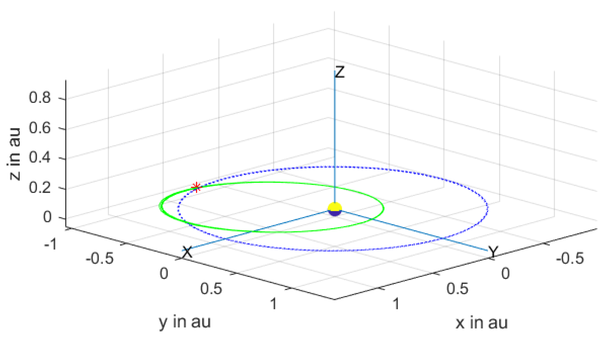
Initially, the satellite is assumed to be orbiting the Earth at the edge of the Earth’s SOI. Following the application of a ‘$\mathsf{\Delta }v$’ impulse the satellite is on a transfer orbit till it intersects the asteroid’s orbit plane where, following a plane change, the satellite is orbiting the Sun in the same plane as the asteroid. This initial phase of the satellite’s orbit is shown in Figure 1.

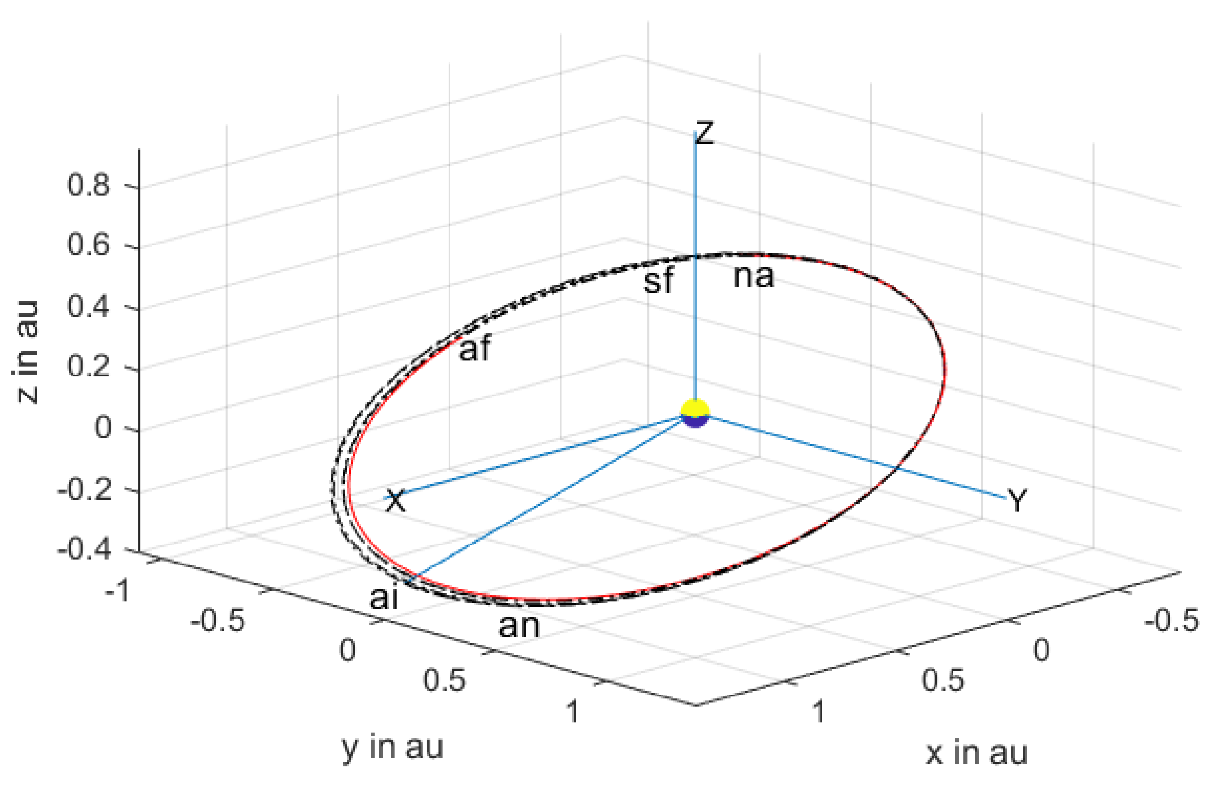
In Figure 1, the descending node is shown both on the satellite’s orbit by a ‘*’. The satellite’s orbit after the plane change is shown in Figure 2. (The preceding orbits are not shown for clarity). The initial location of the asteroid is shown by ‘ai’. When the satellite is at the descending node, the asteroid is at ‘an’. At the end of the simulation of these phases the satellite is at ‘sf’ while the asteroid is at ‘af’. At this juncture, the satellite is sufficiently close to the asteroid to make it feasible for the synthesis of the optimal trajectory during the powered phase. In Figure 3, are shown the trajectory of the satellite and the orbit of the asteroid, after the start of the powered phase and beyond. (The preceding orbits are not shown for clarity). The end of these phases is shown as ‘na’ and on this last phase the satellite and asteroid are co-located.

The control accelerations used to generate the optimal trajectory were generated using the original HCW Equation (54), the adjoint Equation (61) with the co-state boundary conditions (63) and the control Equation (62) and are shown in Figure 4. In this simulation, example both R and Q_f in Equation (59) are chosen to be identity matrices.

It may be observed that the time frame required for the satellite to catch up with the asteroid was just under 700 h. The time histories of the position and velocity coordinates corresponding to the control accelerations in Figure 4, are shown in Figure 5. In Figure 6 is shown the time history of the distance of the satellite relative to the asteroid as well as the x-y plane orbit of the position of the satellite relative to the asteroid.

The control accelerations are now recomputed and used to generate the optimal trajectory were generated using the alternate HCW Equation (64) in terms of the secular relative orbital motion states, the adjoint Equation (69) with the co-state boundary, Condition (71) and the control, Equation (70). In the simulation both R and Q_fr in Equation (68) are chosen to be identity matrices. In Figure 7 are shown the corresponding trajectory of the satellite and the orbits of the Earth and asteroid, including the powered phase and beyond. The end of these phases is shown as ‘na’ and on this last phase the satellite and asteroid are co-located. It may be observed that the time frame required for the satellite to catch up with the asteroid is now just under 2560 h.

There are indeed several differences between the two sets of results, shown in Figure 4, Figure 5, Figure 6 and Figure 7 and Figure 8, Figure 9, Figure 10 and Figure 11, although Figure 6 and Figure 10 are apparently similar. The most significant differences are in the optimal control accelerations computed using the two sets of representations, shown in Figure 4 and Figure 8.

For the initial and final conditions under which the optimal controls were computed, the maximum control accelerations are 100 times lower when Equations (64), (69) and (70) are used although the time frame required has almost tripled. Moreover, the behavior of both components of the control accelerations in the LVLH frame, is monotonic when Equations (64), (69) and (70) are used and not monotonic when Equations (54), (61) and (62) are used. However, the overall mission time was 2.7 years when Equations (64), (69) and (70) are used and 2.49 years when Equations (54), (61) and (62) are used.

A search of feasible trajectories showed that it was indeed possible to reduce the total mission time to 2.67 years albeit with an increase in the control accelerations almost by a factor of ten. The time frame over which the control acceleration was deployed reduced to just under 2300 h. In Figure 11, the control acceleration was deployed about 36 days, earlier than in Figure 7. The general nature of the time histories of the control accelerations and relative positions and velocities in Figure 10 and Figure 11 was similar to those shown in Figure 6 and Figure 7.

While the effect of the quadrupole moment coefficients of the central bodies were included in all the trajectory simulations, the control accelerations were computed both with and without these oblateness effects to ensure that the control accelerations in both cases were not significantly different. No significant differences were found in the control accelerations with the effect of the quadrupole moment coefficients of the central bodies included.

9. Discussions and Conclusions

In this paper, it has been clearly demonstrated that the choice of the state space representation can have a significant impact on the optimal trajectories that can be synthesized when considering the relative motion orbits of two orbiting bodies. This is quite understandable as the state representations are essentially approximations to the relative motion dynamics and it is indeed plausible that one representation leads to better approximation to the feasible optimal trajectory than the other. In particular, in the case of the HCW equations, the existence of two different time scales in the solutions, requires that the reduction to a state space is done carefully, separating the solutions with different time scales. Although the existence of multiple time scales has been recognized in the past by a few authors, the particular reduction to state space form has not been employed in the past for optimal trajectory synthesis.

One important application of the relative motion dynamics is to the problem of a satellite seeking to fly in close proximity to an asteroid. Thus, using this problem as a bench marking example, it has been demonstrated that significant reductions in the magnitudes of the control accelerations can be achieved by choosing the right state representation of the approximate dynamics of the relative motion. It must be said that the methodology could be applied to host of other problems, where it is essential to synthesize an optimal trajectory to another orbiting body in close proximity to a satellite. However, it is expected that the methodology will be most useful in designing optimal low-impulse trajectories for flying in close proximity to a host of other asteroids. Once this is done, the delivery of an optimum impulse to deflect the asteroid is feasible. This facilitates several deep space missions requiring control continuous thrust deployment. Thus, the methodology developed can have a significant impact on the design of low thrust trajectories of the satellites which are equipped by electric thrusters.