Three-Phase Symmetric Distribution Network Fast Dynamic Reconfiguration Based on Timing-Constrained Hierarchical Clustering Algorithm

Abstract

This paper develops a novel dynamic three-phase symmetric distribution network reconfiguration (DNR) approach based on hierarchical clustering with timing constraints, which can divide the time period according to the time-varying symmetric load demand and symmetric distributed generations (DGs) output condition for a given time interval. The significance of the proposed technique is that by approximating the cluster center as the load status and DGs output status of the corresponding period, in this way, the intractable dynamic reconfiguration problem can be recast as multiple single-stage static three-phase symmetric DNR problems, which can effectively reduce the complexity of the three-phase symmetric dynamic reconfiguration. Furthermore, an improved fireworks algorithm considering heuristic rules (H-IFWA) is proposed and investigated to efficiently manage each single-stage static three-phase symmetric DNR problem. In order to avoid trapping into a local optimum or to facilitate the computational performance, the power moment method and the coding method based on heuristic rules are employed to reduce the solution space. The effectiveness of the proposed H-IFWA is validated on the IEEE 33, 119-bus system and a practical-scale Taiwan power company (TPC) 84-bus test system with DGs.

1. Introduction

Distribution network reconfiguration (DNR) is the process of changing the topology of a network by switching the status of the tie switch and the section switch for the purpose of reducing the network loss, balancing load and improving voltage quality, and it is of great significance to improve the safe and economic operation of distribution networks (DNs) [1,2,3]. DNR is usually divided into two types [4]: DNR in the normal operation status and DNR after an accident [5]. DNR in the normal operation status further consists of two types: static reconfiguration [6,7] and dynamic reconfiguration [8,9,10]. The former optimizes the section switches and tie switches of the distribution network based on the premise that the load does not change [11]. The latter performs the overall dynamic optimization of the distribution network during the operation periods [12], which needs to consider the time-varying load demand and the constraints of the distribution network operation for a given time interval [13]. Considering the time-varying system condition in the real distribution system, this paper focuses on dynamic DNR in the normal operation status. Furthermore, symmetry in DNR means that the power source and load are the three-phase circuit, and both of them are symmetrical in the reconfigured distribution network.

Renewable energy sources have been actively applied to distribution networks and microgrids for better energy management, including residential buildings [14], logistics facilities [15], and network reconfiguration [16]. Nevertheless, the deepening penetration of renewable distributed generations (DGs), such as wind and solar resources, has significantly changed the characteristics of distribution networks. The traditional one-way power flow three-phase symmetric distribution network analysis method cannot be applied to the current two-way power flow three-phase asymmetric active distribution network with multiple distributed renewable sources, which makes the DNR problem face more complex challenges on the power flow calculation [17], fault recovery [5,18], and optimal reconfiguration [19,20,21] of distribution networks. Therefore, dynamic DNR considering the massive integration of DGs is of great significance to develop the operation level of the distribution network and the utilization efficiency of DGs. Dynamic DNR takes into account such factors as power loss, switching times, and comprehensive cost within a certain period, which can effectively adjust the topology of the distribution network in real time with the time-varying load demand and DGs output condition. Therefore, the research on dynamic DNR has become the current research hotspot.

In recent years, many studies have addressed the ever-increasing concern for solving the dynamic DNR problem. In [22], a mixed-integer nonlinear programming method was presented to solve the problem of dynamic reconfiguration and optimal allocation of capacitors, but the time period division method was not involved. As an extension of the fascinating DNR method, [23] considered the time-varying intermittence of DGs, but the restrictions of switching operation times were not taken into account. In [24], a gradual approaching method was developed for dynamic DNR to minimize the energy loss. In [25], an evolutionary method to determine optimal time intervals was proposed, and the genetic algorithm was applied to perform optimal dynamic DNR. These methods have considered both the time-varying load demand and DGs power output condition in a given time interval. In [26], a real-time dynamic reconfiguration method using load power analysis and the analytic hierarchy process (AHP) to generate multi-criteria decision-making was proposed; however, the limitation of switching operation times was not considered. In [27], the optimal solution in each period, respectively, was determined, and then rules were formulated to obtain a globally optimal solution, but the solution process was complicated and it was difficult to guarantee the speed of optimization. In [28], an optimal fuzzy C-means clustering was employed to divide time periods, but the rationality of the partition results may be insufficient, which may restrict the accuracy of the solution and produce large errors.

To handle the aforementioned challenges, in this paper, considering the output condition of DGs and load status, a time-division method based on an improved hierarchical clustering with timing constraints (IHCTC) algorithm is firstly proposed. According to the load status and DGs output of each period, the time is divided by adding the timing constraints to the Euclidean distance between data points in hierarchical clustering. In this way, the dynamic DNR problem is recast as a multiple single-stage static DNR problems, and it satisfies the switching number constraints. Then, an improved fireworks algorithm considering heuristic rules (H-IFWA) is developed to handle single-stage static DNR for the clustering center. Finally, case studies are carried out on the modified IEEE 33, IEEE 119 and a practical scale TPC 84-bus test systems to validate the effectiveness of the proposed method. The main contributions are summarized as follows:

(1)

A novel time-division method based on hierarchical clustering with timing constraints, which can ensure the rationality of the time-division method, is firstly proposed to solve the statics of the dynamic reconfiguration problem.

(2)

An improved fireworks algorithm considering heuristic rules (H-IFWA), for the first time, is presented, which can both improve the solving speed of DNR and avoid falling into a local optimum or producing many infeasible solutions.

The remainder of the paper is organized as follows. An improved hierarchical clustering with timing constraints method is described in Section 2. Then, a three-phase symmetric dynamic reconfiguration model with the objective of minimizing the total active power loss is formulated in Section 3. Section 4 introduces the H–IFWA method. Several case studies are conducted in Section 5 to demonstrate the superior performance of the proposed H–IHCTC and IFWA algorithms, and the conclusions are drawn in Section 6.

2. Hierarchical Clustering with Timing Constraints

Hierarchical clustering (HC) creates a hierarchical nested clustering tree in light of the similarity calculation between different categories of data points. The basic steps are as follows. The basic steps are described in our previous work [29].

Step 1: Regard each data point as a class, and calculate the minimum distance between any two classes.

Step 2: Seek the smallest distance between the two classes, and then combine them into a new class.

Step 3: Repeat Step 1 to obtain the distance between the new class and all remaining classes.

Step 4: Repeat Step 2 and Step 3, terminate the calculation, and output the result when all the classes are merged into a single class.

Here, we use Euclidean distance to calculate the similarity of data points [29].

The load of the distribution system at different times affects the quality of operation indexes such as network loss to a great extent, which is also an important basis for DNR operation. Therefore, we take the load data of each natural period of the day (one hour) as sample points for hierarchical clustering. The daily load data of the three-phase symmetric distribution network in a certain area are clustered, and the results are shown in Figure 1a. If the number of clusters is 3, the corresponding three categories are {1–6, 18–24}, {7–8, 17}, and {9–16}, respectively. Obviously, except for the last category, which is continuous in time, the other two are not continuous, so it is difficult to apply it to the time-division problem of dynamic reconfiguration.

To keep each category continuous in time, we redefine the Euclidean distance d_i,j between data points as:

$$d_{i,j}=\{\begin{array}{cc}\sqrt{{\displaystyle \sum _{k=1}^n{(x_{i,k}-x_{j,k})}^2}}\hfill & ,\left|i-j\right|\le 1\hfill \\ +\infty \hfill & ,\left|i-j\right|>1\hfill \end{array} ,x_i,x_j\subset D$$

(1)

where n represents data points’ dimension and D denotes all data points’ set.

The abovementioned definition means that only two adjacent data points can be grouped into one cluster, so that the time sequence constraints of time-division can be considered. According to the definition, HCTC is implemented for the same daily load data, and the result is shown in Figure 1b. If we take the number of clusters as 3, the three categories obtained are {1–6}, {7–17}, and {18–24}. It can be seen that the HCTC method can obtain continuous clustering results in time, which meets the actual needs of time-division in DNR.

However, when the clustering number takes other values, undesired results may be obtained through HCTC. For example, when the number of clusters is 5, the clustering results are {1–6}, {7–8}, {9–16}, {17}, and {18–24}. When DNR is performed according to the clustering result, there will be two reconfiguration operations between 16 h and 18 h, which is obviously unreasonable and will lead to frequent switch actions.

To solve the above problems, an IHCTC method is proposed. The basic idea is to view the clustering process as an optimization problem, and its objective function is:

$$\min F(T_d)={\displaystyle \sum _{t=1}^{T_d}{\displaystyle \sum _{h=1}^{H_t}{d}_{h,avi}^t}},\begin{array}{cc}& T_{\min }\le T_d\le T_{\max },H_t\ge H_{\min }\end{array}$$

(2)

where F depicts the inner-distance of class, T_max and T_min are the maximum and minimum number of periods, T_d means divided periods’ number, H_t represents hours’ number in period t, H_min describes the shortest duration allowed for each period, and $d_{h,avi}^t$ represents the proposed Euclidean distance from the h-th hour during period t to the clustering center, which can be expressed as:

$$d_{h,avi}^t=\sqrt{{\displaystyle \sum _{k=1}^n{(x_{h,k}^t-\overline{X_t})}^2}}$$

(3)

where $\overline{X_t}$ denotes the clustering center of the t-th period.

Considering that the abovementioned optimization problem is a single variable discrete optimization problem in a finite interval, the enumeration method is adopted to solve it. As illustrated in

Table 1. Clustering results based on IHCTC.

Td	2	3	4	5
Time interval	1–6; 7–24	1–6; 7–17; 18–24	7–17; 18–21; 22–24	1–5; 6–8; 9–17; 18–21; 22–24
Inner-distance F	8.19	5.43	4.80	4.45

, based on the IHCTC method, the same daily load data are analyzed.

It can be seen from Table 1 that, as T_d increases, the inner-distance F decreases gradually, and there are no isolated data points. When DNR is performed according to the clustering result, there will be no problem of frequent switch action.

3. Three-Phase Symmetric Dynamic DNR Model

The DNR optimization goal is the minimum total network losses in the optimization period, which can be expressed as:

$$\min {\displaystyle \sum _{t=1}^{T_d}{\displaystyle \sum _{l=1}^{N_L}\frac{P_{l,t}^2+Q_{l,t}^2}{V_{l,t}^2}{r}_l{H}_t}}$$

(4)

where N_L represents the branches’ set, r_l represents branch resistance, V_l,t represents the voltage amplitude of the terminal node of branch l at period t, and P_l,t and Q_l,t are the active power and reactive power at the end of branch l at period t, respectively.

To ensure that the solution of the DNR problem is feasible, the following constraints need to be considered.

(1) Power balance constraint

$$S_{i,t}^{\prime }=S_{L,i,t}-S_{G,i,t}+{\displaystyle \sum _{j=1}^k{S}_{i,j,t}},\begin{array}{cc}& i=1,2,\cdots ,N_L; t=1,2,\cdots ,T_d\end{array}$$

(5)

$$S_{i,t}=S_{i,t}^{\prime }+\Delta S_{i,t},\begin{array}{cc}& i=1,2,\cdots ,N_L; t=1,2,\cdots ,T_d\end{array}$$

(6)

where $S_{i,t}$ and $S_{i,t}^{\prime }$ are the complex power of the start node and the end node of branch i in period t, respectively, $S_{L,i,t}$ is the load power of the end node of branch i in period t, $S_{G,i,t}$ is the injection power of the DG connected to the end node of branch i in period t, $S_{i,j,t}$ is the complex power of the j-th out-branch of the end node of branch i in period t, and $\Delta S_{i,t}$ is the complex power consumed by branch i.

(2) Node voltage constraints

The voltage of node i in any period t should meet:

$$\min \left(V_{i,t}|i=1,2,\cdots ,N_B; t=1,2,\cdots ,T_d\right)\ge V_{\min }$$

(7)

$$\max \left(V_{i,t}|i=1,2,\cdots ,N_B; t=1,2,\cdots ,T_d\right)\le V_{\max }$$

(8)

where N_B represents nodes’ number in the distribution network, and V_min/V_max are the allowable minimum/maximum values of node voltage, respectively.

(3) Branch capacity constraint

Limited by the maximum allowable carrying capacity, the power S_i,t of branch i in any period t should meet:

$$S_{i,t}\le S_i^{\max }\begin{array}{cc}& i=1,2,\cdots ,N_L; t=1,2,\cdots ,T_d\end{array}$$

(9)

where $S_i^{\max }$ represents the rated capacity of branch i.

(4) Network topology constraints

The reconstructed network should meet [8]:

$${\displaystyle \sum _{k\in {\Omega }_B}^{}{\alpha }_k=N_B-1}$$

(10)

$$\beta (i,j)+\beta (j,i)={\alpha }_k$$

(11)

$${\displaystyle \sum _{j\in \Omega (i)}\beta (i,j)=1}$$

(12)

$$\beta (i,j)\in \{0, 1\},i=1,2,\dots ,N_B,j\in \Omega (i)$$

(13)

$${\alpha }_k\in \{0, 1\},\begin{array}{cc}& \end{array}k=1,2,\cdots ,N_L$$

(14)

where ${\alpha }_k$ is the 0–1 variable that reflects the status of branch k; ${\alpha }_k=1$ indicates that the branch is connected. Otherwise, the branch is opened. $\beta$ represents the node child–parent correlation matrix, in which the elements are all binary variables; if $\beta (i,j)=1$, it means that the node i is the parent node of node j. $\Omega (i)$ represents a collection of all nodes connected to node i.

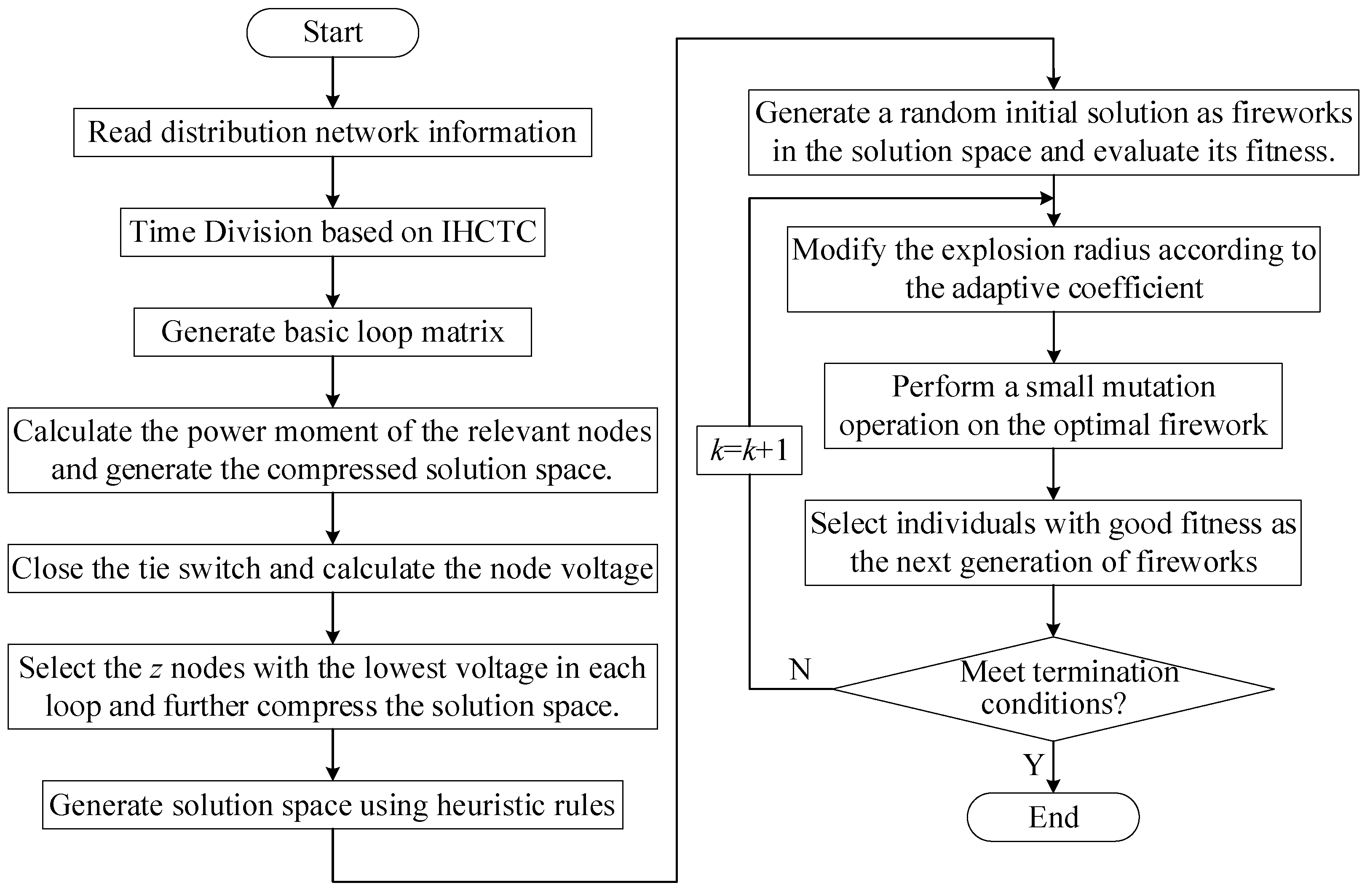
4. Solution Algorithm

4.1. Solution Space

Due to the fact that the proposed three-phase symmetric dynamic DNR model is a nonlinear integer programming problem, a heuristic method is employed to solve it to improve the solution efficiency. Motivated by this, we first describe the solution space of the model. Considering the characteristics of the open-loop DN operation, one switch in each loop must be in the open status (tie switch), and the other switches are in the closed status (section switch). When the status of the tie switch and a section switch is reversed, a new radial topology is obtained. Therefore, we use the loop as the unit and use a matrix to describe the topology of the DN. Take the 16-bus system [30] shown in Figure 2 as an example.

The network consists of three source points (node 1~node 3) and 16 branches with switches. Each tie switch in the open status corresponds to a loop, so the network contains three loops. The branches contained in each loop are arranged to form the following basic loop matrix.

$$S_{p0}^{}=\left[\begin{array}{ccccccc}1& 2& 5& 6& 8& 14& 0\\ 5& 7& 10& 11& 15& 0& 0\\ 1& 3& 4& 10& 12& 13& 16\end{array}\right]$$

(15)

Selecting one branch from each row of S_p0, and taking the corresponding switches as the tie switches and the other switches as the section switches, then a three-phase symmetric distribution network topology can be obtained, so the matrix S_p0 can be regarded as the solution space of DNR.

Because there are repeated elements between the rows of the basic loop matrix S_p0, the random selection of branches may lead to invalid solutions. For example, when selecting {5, 5, 1}, that is, branch B5 and branch B1 are opened and other branches are closed, the corresponding network topology is a loop network, which does not meet the constraints (10)~(14), so the solution is invalid. Hence, we use the power moment method [31] to filter the repeated elements of each row in the matrix S_p0 so as to obtain the compressed solution space $S_p^{\prime }$.

$$S_p^{\prime }=\left[\begin{array}{cccccc}2& 8& 6& 14& 0& 0\\ 7& 5& 11& 10& 15& 0\\ 4& 3& 1& 13& 12& 16\end{array}\right]$$

(16)

In addition, some studies [32] have shown that for a certain loop of the three-phase symmetric distribution network, opening the branch connected to the lowest voltage point and closing the original tie switch can most effectively reduce the active power loss of the loop. To further compress the solution space without losing the optimal solution as much as possible, a heuristic rule is proposed, which selects the z nodes with the lowest voltage in each loop, and then the branch set of the loop network is replaced by the branches connected to these nodes in the loop matrix, thereby effectively compressing the solution space.

Taking the system shown in Figure 2 as an example, we close the switches B14, B15, and B16 and perform power flow calculation. The voltage of each node can be calculated and sorted from low to high as:

$$12<9<11<5<7<8<6<16<10<15<14<4<13<3=2=1$$

(17)

Then, we set z = 2; in other words, we select the two lowest voltage nodes in each loop and find their adjacent branches, as illustrated in

Table 2. Selected branches in each loop.

Loop Number	Tie Switch	Lowest Voltage Node	Adjacent Branches	Second Lowest Voltage Node	Adjacent Branches
1	B14	9	B6, B8, B9	11	B8, B14
2	B15	8	B5, B6, B7	10	B7, B15
3	B16	7	B4, B16	6	B3, B4

.

It can be seen from Table 2 that the branches that are not in the corresponding loop are removed. For example, in the branch set {B6, B8, B9}, B9 is not in loop 1, so it should be removed. Then, the branch matrix (solution space) can be obtained.

$$S_p=\left[\begin{array}{ccc}6& 8& 14\\ 5& 7& 15\\ 3& 4& 16\end{array}\right]$$

(18)

The solution space is obviously reduced compared to $S_p^{\prime }$. According to [30], the optimal solution of the symmetric distribution network is {B8, B7, B16}, which is still in $S_p$. The essence of this heuristic rule is to find the most promising branch for reducing the power loss in each loop, thereby filtering out numerous poor solutions.

4.2. Improved Fireworks Algorithm

The fireworks algorithm [33,34] shows excellent global optimization performance and computational efficiency in solving complex optimization problems. The number of sparks produced by the fireworks explosion is negatively correlated with the explosion radius. Based on the enlightenment of this relationship, the FWA seeks the optimal solution space iteratively. First of all, in the solution space, we randomly select the initial solution as the fireworks and evaluate its fitness. It is considered that the fireworks with small explosion radius and more sparks are regarded as good; otherwise, the fitness is poor. The sparks that do not meet the constraints should be modified. After comprehensive evaluation, a new generation of fireworks is obtained, and the abovementioned steps are performed in turn. In each iteration, we select the fireworks that have the best fitness as the optimal fireworks, and the best fireworks y(k) are selected through k iterations, which is the optimal solution.

Dynamic DNR is a nonlinear, discrete and multi-constrained NP problem, and based on this, we propose an IFWA. According to Equation (4), the fitness function of the fireworks algorithm is taken as the DN active power loss. It is assumed that the fitness of the optimal fireworks of the k-th iteration is y(k).

$$y(k-1)\ge y(k)\begin{array}{cc}& \end{array}k\ge 2,k\in Z$$

(19)

where Z is a set of integers greater than 0.

The adaptive coefficient β is defined to represent the survival generations of the optimal fireworks under the current iteration. When the optimal fitness of the first iteration or two adjacent iterations is different, the survival generation is 0. When the optimal fitness of two adjacent iterations is equal, the survival generation is increased by one. Therefore, β is an adaptive coefficient, which can better reflect the search status of the current algorithm.

$$\beta =\{\begin{array}{cc}0\hfill & k=1,y(k-1)>y(k)\hfill \\ \beta +1\hfill & y(k-1)=y(k)\hfill \end{array}$$

(20)

The explosion operator is an important part of the fireworks algorithm that determines the search range and search granularity of the algorithm. To further facilitate the optimization ability of the fireworks algorithm, the explosion radius is improved by the adaptive coefficient in the iterative process. On the one hand, to promote the local search capability, A_opt of the optimal fireworks decreases gradually with the increase in β. On the other hand, to avoid falling into the local optimization, with the increase in β, the explosion radius A_other of non-optimal fireworks is gradually increased. The above process can be expressed as:

$$\{\begin{array}{l}{A}_{opt}^{\prime }=A_{opt}\frac{M}{(M+\beta )}\\ A_{other}^{\prime }=A_{other}\frac{(M+\beta )}{M}\end{array}$$

(21)

where M is a constant, $A_{opt}$ and $A_{other}$ are the optimal and non-optimal fireworks explosion radius before improvement, respectively, and $A_{opt}^{\prime }$ and $A_{other}^{\prime }$ are the optimal and non-optimal fireworks explosion radius after improvement, respectively.

When the explosion radius is decreased to a very small value, the rounded solution is the same as the original solution, that is, there is an invalid variation. To avoid this case, the explosion radius given by Equation (22) is further adjusted, and the explosion radius is set to an integer that is not less than 1.

$$A^{″}=\{\begin{array}{cc}round\left(A^{\prime }\right)\hfill & ,A^{\prime }\ge 0.5\hfill \\ 1\hfill & ,A^{\prime }<0.5\hfill \end{array}$$

(22)

where $A^{\prime }$ and $A^{″}$ are the fireworks explosion radius before and after rounding, respectively. round () is the rounding function.

In the FWA, while iteration times reach the maximum, the algorithm ends and the optimal fireworks are selected as the final solution. If the optimal fireworks obtained after k iterations (not the maximum number of iterations) continuously survive a certain generation C that is large enough, then the optimal fireworks can be considered as the final solution. To ensure the rapidity and accuracy of optimization, it is assumed that C is a large termination constant. So, the improved termination strategy is:

$$V\ge Cork\ge k_{\max }$$

(23)

With the progress of the iterative process, when the explosion radius is reduced to a certain extent, each explosion may produce a large number of the same sparks, thus affecting the search ability of the algorithm. Inspired by this, we implement a small mutation strategy that performs an explosion in each dimension for current optimal fireworks R_opt, thus a new spark is generated and the other dimensions remain unchanged during the operation. The spark R_j generated on the j-th dimension can be expressed as:

$$R_j=R_{opt}+\left[(2\lambda -1)\frac{N_j}{3}\right], \lambda \in [0, 1], j=1,2,\cdots ,n$$

(24)

where n represents the dimension of fireworks, λ depicts an arbitrary constant, and N_j denotes the feasible range of fireworks in dimension j.

Through the small mutation operation of the optimal fireworks, a large number of different new solutions can be obtained nearby the current optimal solution, and this effectively promotes the algorithm’s local search capability.

4.3. Dynamic DNR Steps Based on IHCTC and H-IFWA

Dynamic DNR based on IHCTC and H-IFWA is demonstrated in Figure 3, and the detailed steps are as follows.

Step 1: Reading data of DN include distribution lines, transformers, DGs, and loads, etc.

Step 2: Based on the day-ahead load forecasting data and the active power of DGs, the hierarchical clustering method considering timing constraints is proposed to divide the time of the day into several reconfiguration periods, and the load status of the corresponding period is expressed according to the data of the clustering center.

Step 3: According to the operation characteristics and topological structure of the three-phase symmetric distribution network, the basic loop matrix S_p0 is formulated.

Step 4: Using the power moment method to filter the repeated elements of each row in the matrix S_p0, the compressed solution space $S_p^{\prime }$ is obtained.

Step 5: Open the branch connected to the lowest voltage point and close the original tie switch, and calculate the voltage of each node.

Step 6: Choose z nodes with the lowest voltage in each loop based on the heuristic rules, and then the branch set of the loop network is replaced by the branches connecting to these nodes in the basic loop matrix to further compress the solution space.

Step 7: Select the initial solution randomly as fireworks in the solution space, and evaluate its fitness.

Step 8: It is assumed that the explosion radius is an integer of not less than 1, and the explosion radius is modified according to the adaptive coefficient.

Step 9: The explosion operation is performed on each dimension of the current optimal spark according to the small mutation strategy of the optimal fireworks.

Step 10: Select the individuals with good adaptability as the next generation of fireworks.

Step 11: If the termination conditions are met, output all feasible solutions. Otherwise, proceed to the next iteration.

5. Case Studies

To validate the calculated performance of the presented heuristic rule, the IHCTC and H-IFWA algorithm and the modified IEEE 33, IEEE 119 and a practical scale TPC 84-bus test systems are verified as examples on a PC with AMD R7-5800H, 3.2GHz CPU, and a 64-bit operating system. Finally, in the same configuration environment, the H-IFWA method is compared with the ideal dynamic reconfiguration (IDR) and the dynamic reconfiguration method in the literature [35].

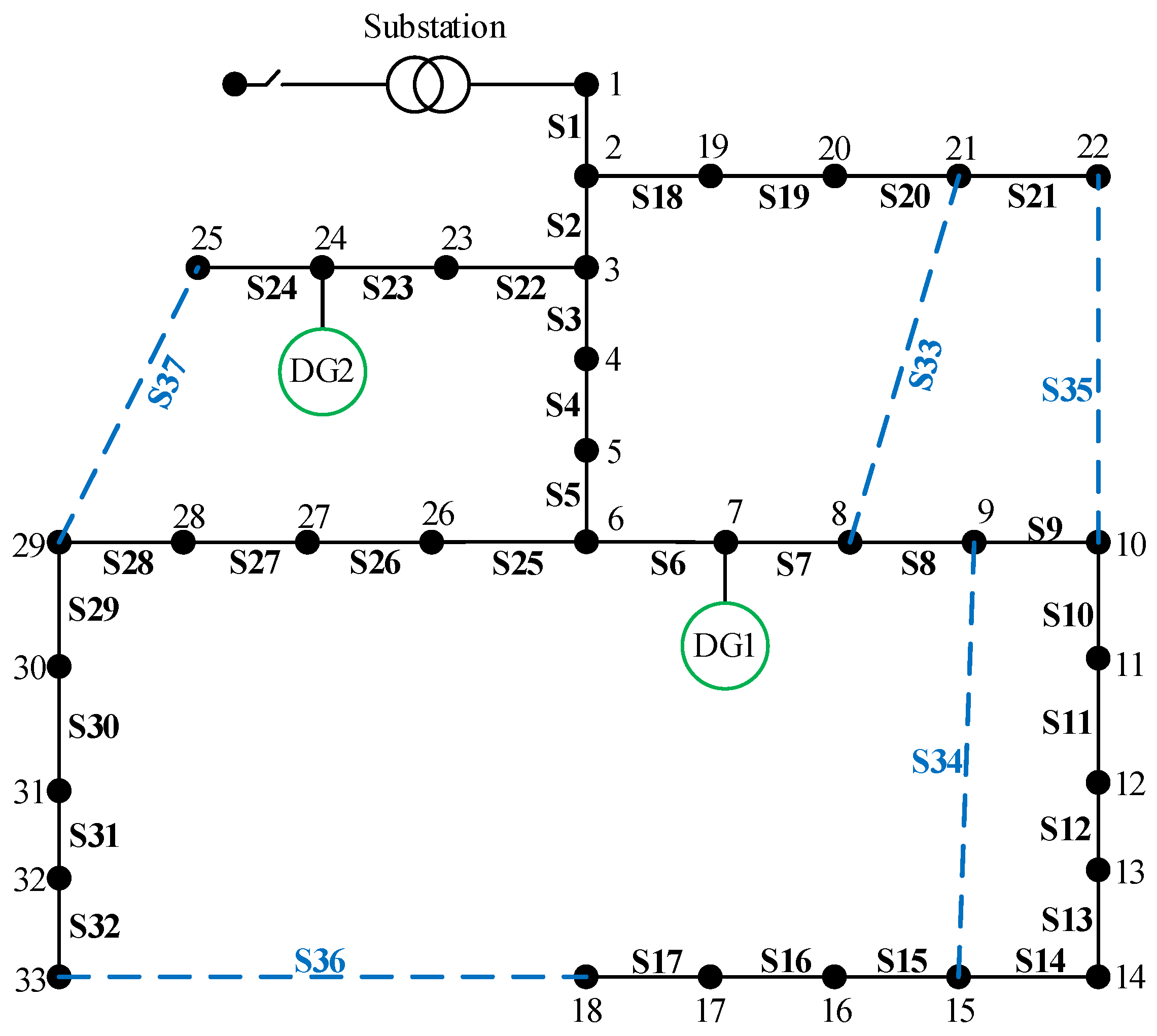
5.1. IEEE-33 Test System

The IEEE-33 test system is shown in Figure 4, and the specific data of the system can be referred to [36]. The DGs are, respectively, installed at node 7 and node 24, and related data are described in

Table 3. Data of DGs.

Node	Rated Active Power (kW)	Rated Reactive Power (kVar)
7	300	240
24	400	360

.

5.1.1. Solution Spaces

To validate that the heuristic rules in the proposed H-IFWA algorithm can effectively reduce the solution spaces, we assume that z = 3, and $S_p$ can be obtained, and this, compared with the results based on the fundamental loop matrix, is displayed in

Table 4. Comparison of solution spaces for IEEE 33-bus system.

Loop	Sp0	Sp
1	{2, 3, 4, 5, 6, 7, 18, 19, 20, 0, 0, 0, 0, 0, 0, 0, 0, 0, 0, 0}	{5, 6, 7, 33}
2	{9, 10, 11, 12, 13, 14, 0, 0, 0, 0, 0, 0, 0, 0, 0, 0, 0, 0, 0, 0}	{12, 13, 14, 34}
3	{2, 3, 4, 5, 6, 7, 8, 9, 10, 11, 18, 19, 20, 21, 0, 0, 0, 0, 0, 0}	{9, 10, 11, 35}
4	{6, 7, 8, 9, 10, 11, 12, 13, 14, 15, 16, 17, 25, 26, 27, 28, 29, 30, 31, 32}	{17, 31, 32, 36}
5	{3, 4, 5, 22, 23, 24, 25, 26, 27, 28, 0, 0, 0, 0, 0, 0, 0, 0, 0, 0}	{24, 27, 28, 37}

.

As can be observed from Table 4, in comparison with the solution space $S_{p0}$, $S_p$ is also significantly reduced, which is due to the fact that the heuristic rule excludes some infeasible solutions so as to reduce the range of solution spaces.

5.1.2. H-IFWA Performance

To demonstrate the superior performance of the proposed H-IFWA algorithm, the comparative analysis results by using the H-IFWA, MILP, FWA [37] and improved harmony search algorithm (IHSA) [38] for 100 times are shown in

Table 5. Comparison of different algorithms.

Items			Original Network	Reconfigured Network
				IHSA	FWA	MILP	H-IFWA
Open switches			B33, B34, B35, B36, B37	B9, B14, B28, B32, B33	B9, B14, B28, B32, B33	B9, B14, B28, B32, B33	B9, B14, B28, B32, B33
Power Loss (kWh)	Best		146.02	94.67	94.67	94.67	94.67
	Worst			99.85	112.25	94.67	94.67
	Average			97.58	102.69	94.67	94.67
Lowest voltage (p.u)			0.9193	0.9490	0.9490	0.9490	0.9490
Average convergence time (s)		Best	--	5.9	6.1	1.8	1.7
		Worst		6.7	6.9	2.3	2.6
		Average		6.1	6.4	1.9	2.1

. The computation time of H-IFWA includes the entire process from the data initialization and the solution time of the algorithm. The computation time of MILP includes the constraint generation time of MATLAB and the solution time of CPLEX.

As can be inferred from Table 5, the identical optimal solution can be obtained by four algorithms, and the average power loss of MILP and H-IFWA is the lowest. However, MILP has the best performance in average convergence time. The main reason is that the linearization technology can simplify the DNR solution process. In addition, both IHSA and FWA use the fundamental loop-based coding method, which has a large solution space and contains numerous invalid solutions. The H-IFWA method greatly reduces the range of the solution space by virtue of heuristic rules, which contains only the most potential branch collection. Therefore, in the IEEE 33-bus system, both MILP and H-IFWA have shown better advantages in convergence performance.

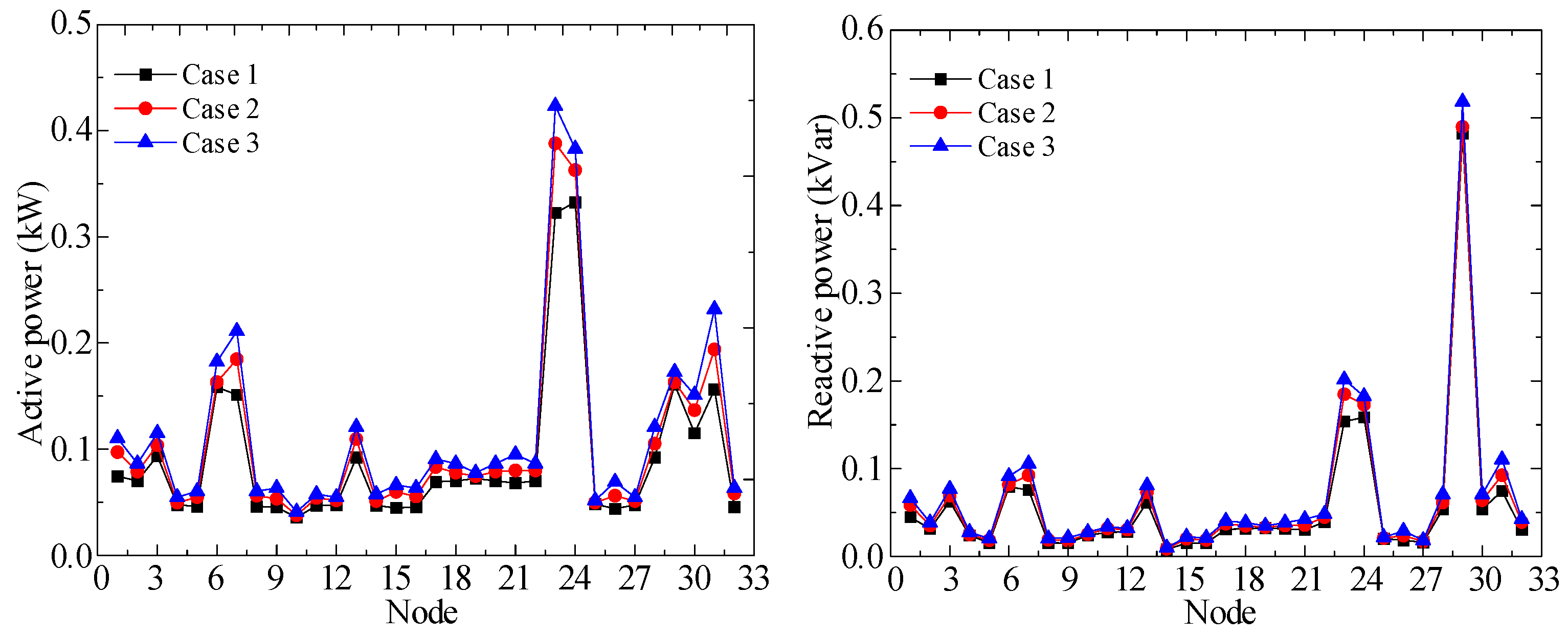
5.1.3. Sensitivity Analysis

To verify the sensitivity of the H-IFWA algorithm proposed in this paper under different load levels, three different load levels are selected to compare the results before and after performing DNR. Here, we take the load levels during three time periods, i.e., 14 h, 19 h, and 21 h, as a case study—this is shown in Figure 5, and the optimization results are illustrated in

Table 6. Comparison of the optimization results for IEEE 33-bus system.

Case	Items	Original Network	H-IFWA
Case 1	Power loss (kWh)	110.29	81.58
	Lowest voltage (p.u)	0.9725	0.9820
Case 2	Power loss (kWh)	143.86	105.52
	Lowest voltage (p.u)	0.9671	0.9785
Case 3	Power loss (kWh)	176.95	128.55
	Lowest voltage (p.u)	0.9629	0.9760

.

As can be seen from Table 6, under three different load levels, the original network loss of three cases is 110.29 kWh, 143.86 kWh, and 176.95 kWh, respectively. After the DNR activity is implemented, the network loss employed in the proposed H-IFWA algorithm is 81.58 kWh, 105.52 kWh, and 128.55 kWh, respectively, which is 26.03%, 26.65%, and 27.35% lower than that of the original scheme. Moreover, the lowest voltage after reconfiguration is higher than that before reconfiguration, so the node voltage level after DNR is obviously improved. Therefore, under three cases by inputting different load values, the H-IFWA method proposed in this paper can effectively reduce power loss and voltage fluctuation in DNR.

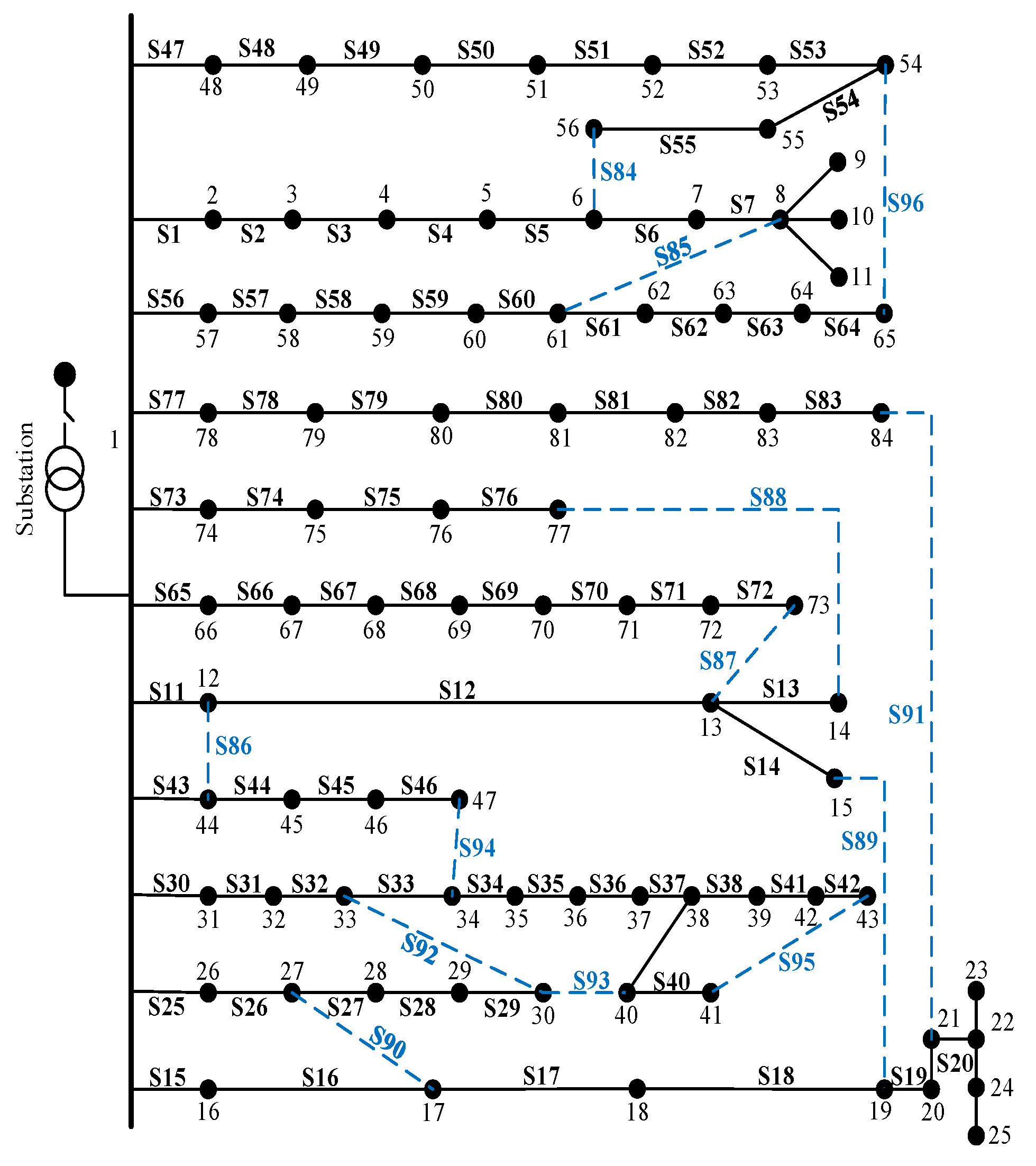
5.2. TPC 84-Bus and IEEE 119-Bus System

The TPC 84-bus system is shown in Figure 6, and the related parameters can be obtained according to [36].

5.2.1. Solution Spaces

To further validate the necessity of heuristic rules in the proposed H-IFWA algorithm, we assume that z = 3, and the solution space $S_p$ can be obtained, and this, compared with the results solved by the fundamental loop matrix, is illustrated in

Table 7. Comparison of solution spaces for TPC 84-bus system.

Loop Number	Sp0	Sp
1	{5, 4, 3, 2, 1, 55, 54, 53, 52, 51, 50, 49, 48, 47, 84, 0, 0}	{5, 54, 55, 84}
2	{7, 6, 5, 4, 3, 2, 1, 60, 59, 58, 57, 56, 85, 0, 0, 0, 0}	{6, 7, 85, 0}
3	{11, 43, 86, 0, 0, 0, 0, 0, 0, 0, 0, 0, 0, 0, 0, 0, 0}	{11, 43, 86, 0}
4	{12, 11, 72, 71, 70, 69, 68, 67, 66, 65, 87, 0, 0, 0, 0, 0, 0}	{70, 71, 72, 87}
5	{13, 12, 11, 76, 75, 74, 73, 88, 0, 0, 0, 0, 0, 0, 0, 0, 0}	{13, 75, 76, 88}
6	{14, 12, 11, 18, 17, 16, 15, 89, 0, 0, 0, 0, 0, 0, 0, 0, 0}	{12, 14 18, 89}
7	{16, 15, 26, 25, 90, 0, 0, 0, 0, 0, 0, 0, 0, 0, 0, 0, 0}	{15, 16, 26, 90}
8	{20, 19, 18, 17, 16, 15, 83, 82, 81, 80, 79, 78, 77, 91, 0, 0, 0}	{80, 81, 82, 83}
9	{28, 27, 26, 25, 32, 31, 30, 92, 0, 0, 0, 0, 0, 0, 0, 0, 0}	{27, 28, 31, 92}
10	{29, 28, 27, 26, 25, 39, 38, 37, 36, 35, 34, 33, 32, 31, 30, 93,0}	{37, 38, 39, 93}
11	{34, 33, 32, 31, 30, 46, 45, 44, 43, 94, 0, 0, 0, 0, 0, 0}	{32, 33, 34, 94}
12	{40, 39, 42, 41, 95, 0, 0, 0, 0, 0, 0, 0, 0, 0, 0, 0, 0}	{40, 41, 43, 95}
13	{53, 52, 51, 50, 49, 48, 47, 64, 63, 62, 61, 60, 59, 58, 57, 56, 96}	{62, 63, 64, 96}

.

It can be concluded from Table 7 that, in comparison with $S_{p0}$, $S_p$ derived from the proposed H-IFWA method is also significantly reduced. Thus, the solving speed of DNR is accelerated. After reconfiguration, the set of open switches is {B55 B7 B86 B72 B13 B89 B90 B83 B92 B39 B34 B42 B62}.

5.2.2. H-IFWA Performance

More importantly, to further explain the superior performance of H-IFWA in the actual TPC 84-bus system, a comparison is made between the proposed H-IFWA, MILP, simulated annealing (SA) [39] and GA for 200 times, and the comparison results are displayed in

Table 8. Comparison of different algorithms for TPC 84-bus system.

Items		Original Network	Reconfigured Network
			SA	GA	MILP	H-IFWA
Power Loss (kWh)	Best	531.99	469.88	469.88	469.88	469.88
	Worst		498.22	489.25	469.88	470.11
	Average		489.82	479.73	469.88	469.89
Lowest voltage (p.u)		0.9193	0.9285	0.9285	0.9285	0.9285
Average convergence time (s)		--	257.43	303.43	9.77	4.86

.

As can be observed from Table 8, in terms of the convergence speed, the H-IFWA method is the best. The main reason is that the solution space of H-IFWA is small and does not require too many iterations, which verifies that H-IFWA has a faster convergence speed. As is shown Table 5, compared with H-IFWA, the solution efficiency of MILP is higher than that in the 33-bus system. However, the number of MILP constraints will gradually increase as the system scale expands, which will increase the constraint processing time and solution time. Therefore, the computation time of MILP is longer than that of H-IFWA in the actual TPC 84-bus system.

Finally, the IEEE 119-bus system [40] is tested to further illustrate the effect of the H-IFWA method compared with the improved tabu search (ITS) [41], harmony search algorithm (HSA) [42], and MILP [40]. The comparison results are listed in

Table 9. Comparison of different algorithms for IEEE 119-bus system.

Items		Original Network	Reconfigured Network
			HSA	ITS	MILP	H-IFWA
Power loss (kWh)	Best	1301.9	865.86	854.21	869.7	869.7
	Worst		1288.1	1282.1	869.7	870.1
	Average		952.6	953.01	869.7	869.8
Lowest voltage (p.u)		0.8783	0.9323	0.9323	0.9383	0.9383
Average convergence time (s)		--	9.04	8.61	11.4	7.36

.

As illustrated in Table 9, the performance of H-IFWA is better than HSA and ITS. The optimal reconfiguration scheme of H-IFWA is {B22 B26 B34 B39 B42 B51 B58 B71 B74 B95 B97 B109 B122 B129 B130}, which is the same as that of MILP. From the comprehensive analysis of Table 5, Table 8 and Table 9, it can be concluded that when dealing with a large-scale DNR problem, H-IFWA has a significant improvement in computational efficiency compared to other algorithms. To sum up, our proposed method has better solving efficiency than existing algorithms, and the reconfiguration scheme is relatively stable.

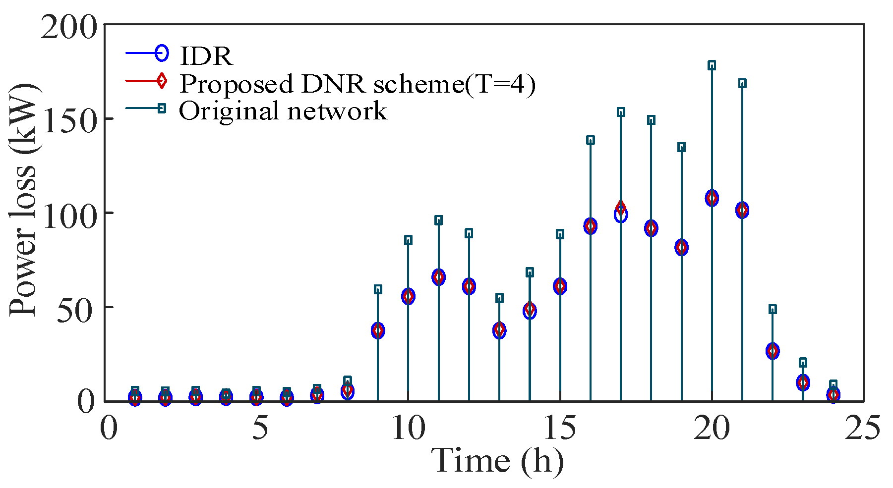
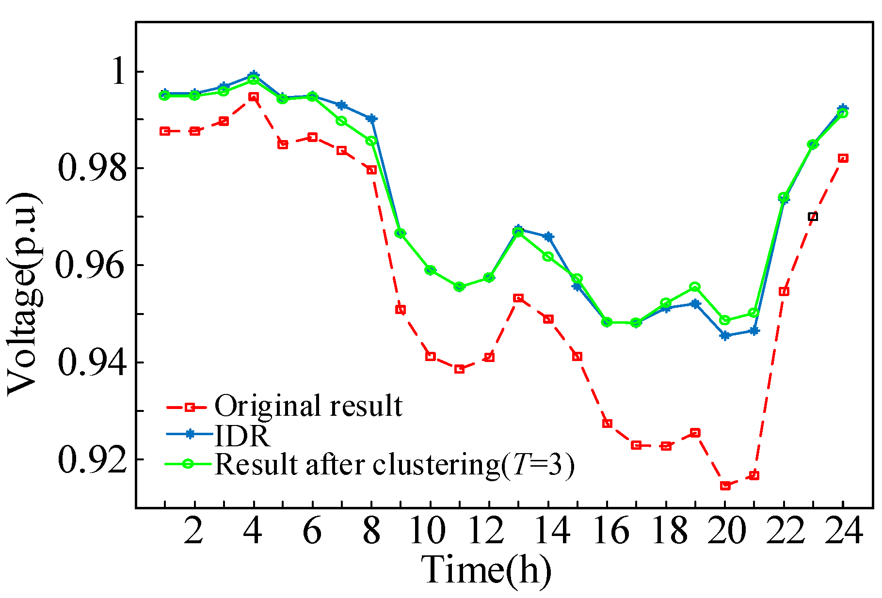
5.3. Comparison with IDR and MPTI Method

DNR is carried out on the IEEE-33 test system by using the daily load data in [43]. In this process, DGs are considered, in which the photovoltaic is connected to node 7 and the wind farm is connected to node 24. The active power of both is illustrated in Figure 7.

5.3.1. Comparison with IDR

To demonstrate the difference between the H-IFWA method proposed in this paper and the ideal dynamic reconfiguration (IDR) method more clearly, according to the combination of single-stage static reconfiguration schemes during 24 periods, an IDR scheme is obtained without considering the limit of switch operation times. The comparison results are shown in Figure 8 and

Table 10. Performance comparison.

Reconfiguration Scheme	Original Network	IDR	H-IFWA
			T = 3	T = 4
Total energy loss (kWh)	1593.99	1003.59	1012.37	1011.76
Saved energy loss (kWh)	0	590.40	581.62	582.23
Energy reduction rate	0	37.04%	36.49%	36.53%
Total number of switch actions	0	33	8	10

, respectively.

From Figure 8 and Table 10, the total energy loss of H-IFWA is 1012.37 kWh (T = 3) and 1011.76 kWh (T = 4), which is 0.87% and 0.81% higher than the total energy loss of IDR, respectively. At the same time, IDR can save energy up to 590.40 kWh, which is higher than H-IFWA by 8.78 kWh (T = 3) and 8.17 kWh (T = 4), respectively. The total energy loss and saved energy loss of H-IFWA are very close to IDR. On the contrary, the number of switching actions of H-IFWA (8 (T = 3) or 10 (T = 4)) is much lower than IDR (33). From these aspects, it is easy to draw the conclusion that H-IFWA can not only meet the DNR constraints, but also significantly reduce the active power loss. Therefore, H-IFWA shows superior performance. In addition, the computation time of IHCTC is 0.28 s, which can meet the engineering requirements of dynamic reconfiguration.

Additionally, the lowest voltages of three dynamic DNR schemes in each period are shown in Figure 9.

As is perceived in Figure 9, the voltage level of the original result is the lowest. In the first segment interval (1–8 h) and the third segment interval (22–24 h), the original network voltage magnitude reaches 0.95 p.u or an even higher voltage magnitude, so the effect of reconfiguration on increasing the voltage magnitude during these periods is not obvious. However, in the second segmentation interval (9–16 h), the lowest voltage of the system in the two reconfiguration schemes is greatly increased. This shows that the two reconfiguration schemes can effectively increase the voltage magnitude.

5.3.2. Comparison with MPTI Method

Furthermore, to validate the superior performance of H-IFWA, DNR is implemented according to the data in [35], in which the membership partition of time intervals (MPTI) method was used, and the comparison results of three schemes are illustrated in

Table 11. Comparison of dynamic reconfiguration schemes.

Reconfiguration Scheme		Time Interval	Open Switches	Energy Loss (kWh)	Saved Energy Loss (kWh)	Loss Reduction Rate
Original network		--	33-34-35-36-37	2217.50	0	0
Literature [35]		1–8	7-9-14-32-37	1540.91	676.59	30.51%
		9–21	7-9-14-32-37
		22–24	7-9-14-32-37
Proposed method	T = 1	1–24	7-9-14-32-28	1530.10	687.40	31.00%
	T = 2	1–16	7-9-14-32-28	1526.65	690.85	31.15%
		17–24	7-9-14-32-37
	T = 3	1–16	7-9-14-32-28	1525.78	691.72	31.19%
		17–21	7-9-14-32-37
		22–24	7-9-14-32-28

.

It is highlighted from Table 11 that the results of the three schemes solved by using the MPTI method in [35] are consistent, which has the same effect as single-stage static reconfiguration. However, the proposed H-IFWA method belongs to dynamic reconfiguration, which can flexibly divide the reconfiguration periods according to actual needs. It is worth mentioning that, with the increase in time-division, the number of reconfiguration schemes also increases, and the energy loss also shows a downward trend. When T = 3, the energy loss is dropped to 1525.78 kWh and the saved energy loss reaches 691.72 kWh. Furthermore, when T = 1, the dynamic reconfiguration result of the H-IFWA method is also better than that of the MPTI method in [35]. Combined with the actual requirements of the distribution network (including power quality and allowable switch operation times), different reconfiguration schemes can be selected appropriately, which further verifies the superiority of the presented algorithm in this paper.

6. Conclusions

In this paper, an improved hierarchical clustering technique based on timing constraints combined with an improved fireworks algorithm is presented to tackle the dynamic DNR problem. Numerical experiments are carried out on three representative IEEE 33, IEEE 119 and TPC 84-bus test systems to verify the effectiveness of the proposed method. The conclusions can be summarized as follows:

(1)

IHCTC is developed to divide periods in terms of the load status and the output condition of DGs, and then the improved fireworks algorithm based on heuristic rules is proposed to recast the intractable dynamic reconfiguration problem as multiple single-stage static reconfiguration problems, which reduces the complexity of dynamic reconfiguration.

(2)

Compared with the advanced algorithms used in the existing literature, the proposed H-IFWA method not only has higher solution efficiency and avoids a large number of invalid solutions, but also can minimize the network loss as much as possible, so it is more suitable for the actual distribution network operation.

However, the practical distribution network usually has voltage-dependent loads, and the uncertainty of DG power can also impact the reconfiguration solutions. Dealing with the uncertainty in a distribution network with voltage-dependent loads and comparing clustering with partitioning methods considered in the solution method [44,45] are the focus of our future research.

References

1. Zhan, J.; Liu, W.; Chung, C.Y.; Yang, J. Switch opening and exchange method for stochastic distribution network reconfiguration. IEEE Trans. Smart Grid 2020, 11, 2995–3007. [Google Scholar] [CrossRef]
2. Badran, O.; Mekhilef, S.; Mokhlis, H.; Dahalan, W. Optimal reconfiguration of distribution system connected with distributed generations: A review of different methodologies. Renew. Sustain. Energy Rev. 2017, 73, 854–867. [Google Scholar] [CrossRef]
3. Mishra, S.; Das, D.; Paul, S. A comprehensive review on power distribution network reconfiguration. Energy Syst. 2017, 8, 227–284. [Google Scholar] [CrossRef]
4. Shi, Q.; Li, F.; Olama, M.; Dong, J.; Xue, Y.; Starke, M.; Winstead, C.; Kuruganti, T. Network reconfiguration and distributed energy resource scheduling for improved distribution system resilience. Int. J. Electr. Power Energy Syst. 2021, 124, 1–10. [Google Scholar] [CrossRef]
5. Jain, T.; Ghosh, D.; Mohanta, D.K. Augmentation of situational awareness by fault passage indicators in distribution network incorporating network reconfiguration. Prot. Control. Mod. Power Syst. 2019, 4, 1–14. [Google Scholar] [CrossRef] [Green Version]
6. Chandrakant, C.V.; Mikkili, S. A typical review on static reconfiguration strategies in photovoltaic array under non-uniform shading conditions. CSEE J. Power Energy Syst. 2020, 1–33. [Google Scholar] [CrossRef]
7. Ajmal, A.M.; Ramachandaramurthy, V.K.; Naderipour, A.; Ekanayake, J.B. Comparative analysis of two-step GA-based PV array reconfiguration technique and other reconfiguration techniques. Energy Convers. Manag. 2021, 230, 113806. [Google Scholar] [CrossRef]
8. Ji, X.; Yin, Z.; Zhang, Y.; Xu, B.; Liu, Q. Real-time autonomous dynamic reconfiguration based on deep learning algorithm for distribution network. Electr. Power Syst. Res. 2021, 195, 107132. [Google Scholar] [CrossRef]
9. Gao, Y.; Wang, W.; Shi, J.; Yu, N. Batch-constrained reinforcement learning for dynamic distribution network reconfiguration. IEEE Trans. Smart Grid 2020, 11, 5357–5369. [Google Scholar] [CrossRef]
10. Azizivahed, A.; Arefi, A.; Ghavidel, S.; Shafie-Khah, M.; Li, L.; Zhang, J.; Catalao, J.P.S. Energy management strategy in dynamic distribution network reconfiguration considering renewable energy resources and storage. IEEE Trans. Sustain. Energy 2020, 11, 662–673. [Google Scholar] [CrossRef]
11. Mukhopadhyay, B.; Das, D. Multi-objective dynamic and static reconfiguration with optimized allocation of PV-DG and battery energy storage system. Renew. Sustain. Energy Rev. 2020, 124, 109777. [Google Scholar] [CrossRef]
12. Ajmal, A.M.; Babu, T.S.; Ramachandaramurthy, V.K.; Yousri, D.; Ekanayake, J.B. Static and dynamic reconfiguration approaches for mitigation of partial shading influence in photovoltaic arrays. Sustain. Energy Technol. Assess. 2020, 40, 100738. [Google Scholar] [CrossRef]
13. Azad-Farsani, E.; Sardou, I.G.; Abedini, S. Distribution network reconfiguration based on LMP at DG connected busses using game theory and self-adaptive FWA. Energy 2021, 215, 119146. [Google Scholar] [CrossRef]
14. Del Granado, P.C.; Wallace, S.W.; Pang, Z. The value of electricity storage in domestic homes: A smart grid perspective. Energy Syst. 2014, 5, 211–232. [Google Scholar] [CrossRef]
15. Wang, Y.; Huang, Z.; Shahidehpour, M.; Lai, L.L.; Wang, Z.; Zhu, Q. Reconfigurable distribution network for managing transactive energy in a multi-microgrid system. IEEE Trans. Smart Grid 2020, 11, 1286–1295. [Google Scholar] [CrossRef]
16. Iris, Ç.; Lam, J.S.L. A review of energy efficiency in ports: Operational strategies, technologies and energy management systems. Renew. Sustain. Energy Rev. 2019, 112, 170–182. [Google Scholar] [CrossRef]
17. Uniyal, A.; Sarangi, S. Optimal network reconfiguration and DG allocation using adaptive modified whale optimization algorithm considering probabilistic load flow. Electr. Power Syst. Res. 2021, 192, 106909. [Google Scholar] [CrossRef]
18. Kahouli, O.; Alsaif, H.; Bouteraa, Y.; Ben Ali, N.; Chaabene, M. Power system reconfiguration in distribution network for improving reliability using genetic algorithm and particle swarm optimization. Appl. Sci. 2021, 11, 3092. [Google Scholar] [CrossRef]
19. Aziz, T.; Lin, Z.; Waseem, M.; Liu, S. Review on optimization methodologies in transmission network reconfiguration of power systems for grid resilience. Int. Trans. Electr. Energy Syst. 2021, 31, 12704. [Google Scholar] [CrossRef]
20. Yin, Z.; Ji, X.; Zhang, Y.; Liu, Q.; Bai, X. Data-driven approach for real-time distribution network reconfiguration. IET Gener. Transm. Distrib. 2020, 14, 2450–2463. [Google Scholar] [CrossRef]
21. Samman, M.A.; Mokhlis, H.; Mansor, N.N.; Mohamad, H.; Suyono, H.; Sapari, N.M. Fast optimal network reconfiguration with guided initialization based on a simplified network approach. IEEE Access 2020, 8, 11948–11963. [Google Scholar] [CrossRef]
22. Pfitscher, L.L.; Bernardon, D.P.; Canha, L.N.; Montagner, V.F.; Garcia, V.J.; Abaide, A.R. Intelligent system for automatic reconfiguration of distribution network in real time. Electr. Power Syst. Res. 2013, 97, 84–92. [Google Scholar] [CrossRef]
23. Sun, X.; Qiu, J. Two-stage volt/var control in active distribution networks with multi-agent deep reinforcement learning method. IEEE Trans. Smart Grid 2021, 12, 2903–2912. [Google Scholar] [CrossRef]
24. Yang, H.P.; Peng, Y.Y.; Xiong, N. Gradual approaching method for distribution network dynamic reconfiguration. In Proceedings of the 2008 Workshop on Power Electronics and Intelligent Transportation System (PEITS), Guangzhou, China, 2–3 August 2008; pp. 257–260. [Google Scholar]
25. Milani, A.E.; Haghifam, M.R. An evolutionary approach for optimal time interval determination in distribution network re-configuration under variable load. Math. Comput. Model. 2013, 57, 68–77. [Google Scholar] [CrossRef]
26. Bernardon, D.P.; Mello, A.; Pfitscher, L.L.; Canha, L.N.; Abaide, A.R.; Ferreira, A. Real-time reconfiguration of distribution network with distributed generation. Electr. Power Syst. Res. 2014, 107, 59–67. [Google Scholar] [CrossRef]
27. Shariatkhah, M.-H.; Haghifam, M.-R.; Salehi, J.; Moser, A. Duration based reconfiguration of electric distribution networks using dynamic programming and harmony search algorithm. Int. J. Electr. Power Energy Syst. 2012, 41, 1–10. [Google Scholar] [CrossRef]
28. Fathabadi, H. Power distribution network reconfiguration for power loss minimization using novel dynamic fuzzy c-means (dFCM) clustering based ANN approach. Int. J. Electr. Power Energy Syst. 2016, 78, 96–107. [Google Scholar] [CrossRef]
29. Zhang, Y.; Ji, X.; Xu, J.; Yin, Z.; Han, X.; Zhang, C. Dynamic reconfiguration of distribution network based on temporal con-strained hierarchical clustering and fireworks algorithm. In Proceedings of the 2020 IEEE/IAS Industrial and Commercial Power System Asia (I&CPS Asia), Weihai, China, 13–15 July 2020; pp. 1702–1708. [Google Scholar]
30. Su, C.-T.; Chang, C.-F.; Chiou, J.-P. Distribution network reconfiguration for loss reduction by ant colony search algorithm. Electr. Power Syst. Res. 2005, 75, 190–199. [Google Scholar] [CrossRef]
31. Ji, X.; Liu, Q.; Yu, Y.; Fan, S.; Wu, N. Distribution network reconfiguration based on vector shift operation. IET Gener. Transm. Distrib. 2018, 12, 3339–3345. [Google Scholar] [CrossRef]
32. Ding, F.; Loparo, K.A. Hierarchical decentralized network reconfiguration for smart distribution systems—Part I: Problem formulation and algorithm development. IEEE Trans. Power Syst. 2015, 30, 734–743. [Google Scholar] [CrossRef]
33. Tan, Y.; Yu, C.; Zheng, S.; Ding, K. Introduction to fireworks algorithm. Int. J. Swarm Intell. Res. 2013, 4, 39–70. [Google Scholar] [CrossRef] [Green Version]
34. Tan, Y. Fireworks Algorithm; Springer Berlin Heidelberg: Berlin/Heidelberg, Germany, 2015; ISBN 978-3-662-46352-9. [Google Scholar]
35. Zhang, K.; Lin, L.; Sun, Y. Dynamic reconfiguration of distribution network based on membership partition of time intervals. Power Syst. Prot. Cont. 2016, 44, 51–57. [Google Scholar]
36. Baran, M.E.; Wu, F.F. Network reconfiguration in distribution systems for loss reduction and load balancing. IEEE Power Eng. Rev. 1989, 9, 101–102. [Google Scholar] [CrossRef]
37. Imran, A.M.; Kowsalya, M. A new power system reconfiguration scheme for power loss minimization and voltage profile enhancement using Fireworks Algorithm. Int. J. Electr. Power Energy Syst. 2014, 62, 312–322. [Google Scholar] [CrossRef]
38. Rajalakshmi, K.; Kumar, K.S.; Venkatesh, S.; Edward, J.B. Reconfiguration of distribution system for loss reduction using improved harmony search algorithm. In Proceedings of the 2017 International Conference on High Voltage Engineering and Power Systems (ICHVEPS), Denpasar, Indonesia, 2–5 October 2017; pp. 377–378. [Google Scholar]
39. Koziel, S.; Rojas, A.L.; Moskwa, S. Power loss reduction through distribution network reconfiguration using feasibility-preserving simulated annealing. In Proceedings of the 2018 19th International Scientific Conference on Electric Power Engineering (EPE), Brno, Czech Republic, 16–18 May 2018. [Google Scholar]
40. Ahmadi, H.; Martí, J.R. Linear current flow equations with application to distribution systems reconfiguration. IEEE Trans. Power Syst. 2015, 30, 2073–2080. [Google Scholar] [CrossRef]
41. Zhang, D.; Fu, Z.; Zhang, L. An improved TS algorithm for loss-minimum reconfiguration in large-scale distribution systems. Electr. Power Syst. Res. 2007, 77, 685–694. [Google Scholar] [CrossRef]
42. Rao, R.S.; Narasimham, S.V.L.; Raju, M.R.; Rao, A.S. Optimal network reconfiguration of large-scale distribution system using harmony search algorithm. IEEE Trans. Power Syst. 2011, 26, 1080–1088. [Google Scholar]
43. Yang, H.; Peng, Y.; Xiong, N. A static method for distribution network dynamic reconfiguration. Power Syst. Prot. Cont. 2009, 37, 53–57. [Google Scholar]
44. Reynolds, A.P.; Richards, G.; de la Iglesia, B.; Rayward-Smith, V.J. Clustering rules: A comparison of partitioning and hierarchical clustering algorithms. J. Math. Model. Algorithms 2006, 5, 475–504. [Google Scholar] [CrossRef]
45. Iris, Ç.; Pacino, D.; Ropke, S.; Larsen, A. Integrated berth allocation and quay crane assignment problem: Set partitioning models and computational results. Transp. Res. Part E Logist. Transp. Rev. 2015, 81, 75–97. [Google Scholar] [CrossRef] [Green Version]
Figure 1. Clustering results of (a) HC and (b) HCTC.
Symmetry 13 01479 g001
Figure 2. A three-feeder symmetric distribution network with 16-bus.
Symmetry 13 01479 g002
Figure 3. Flow chart of dynamic DNR based on IHCTC and H-IFWA.
Symmetry 13 01479 g003
Figure 4. Modified IEEE 33-bus system.
Symmetry 13 01479 g004
Figure 5. Active and reactive power of load under three different conditions.
Symmetry 13 01479 g005
Figure 6. Modified TPC 84-bus system.
Symmetry 13 01479 g006
Figure 7. The daily output of the DGs.
Symmetry 13 01479 g007
Figure 8. Power losses under three dynamic DNR schemes.
Symmetry 13 01479 g008
Figure 9. Lowest voltage under three dynamic DNR schemes.
Symmetry 13 01479 g009