
On Symmetrical Methods for Charged Particle Dynamics


1
School of Mathematics and Statistics, Huazhong University of Science and Technology, Wuhan 430074, China
2
Hubei Key Laboratory of Engineering Modeling and Scientific Computing, Huazhong University of Science and Technology, Wuhan 430074, China
*
Author to whom correspondence should be addressed.
Symmetry 2021, 13(9), 1626; https://doi.org/10.3390/sym13091626
Submission received: 30 July 2021
/
Revised: 12 August 2021
/
Accepted: 13 August 2021
/
Published: 3 September 2021
(This article belongs to the Special Issue Symmetric Methods and Analysis for Time-Dependent Partial Differential Equations)
Abstract
:In this paper, we use the scalar auxiliary variable (SAV) approach to rewrite the charged particle dynamics as a new family of ODE systems. The systems own a conserved energy. It is shown that a family of symmetrical methods is energy-conserving for a new ODE system but may not be for the original systems. Moreover, the methods have high-order accuracy. Numerical results are given to confirm the theoretical findings.
1. Introduction
In this paper, we are interested in investigating high-order numerical methods for solving the following charged particle dynamics [1,2,3,4]:
where and are, respectively, the magnetic and electric fields. In recent years, many energy-conserving numerical methods have been investigated within the framework of line integral methods [1,5] or Runge–Kutta methods [6,7,8,9]. The main results indicate that the method preserves polynomial Hamiltonians. For non-polynomial Hamiltonians, the energy errors appear in the long time simulation. As a result, the numerical methods may not exactly be energy-conserving.
In this short paper, we propose a novel approach to developing some energy-conserving numerical methods for the charged particle dynamics. The main idea can be viewed as an extension of the recent scalar auxiliary variable approach [10,11,12,13,14] or the invariant energy quadratization approach [15]. Firstly, we introduce an auxiliary variable and obtain an auxiliary ordinary differential equation. Together with the original equations (1), we obtain a new family for the ODE system. The new system has the same solution as the original problem (1), and the energy of the new system can be rewritten as the quadratic invariants. Then, we studied the energy-conserving methods in the framework of Runge–Kutta methods. It can be seen that certain Runge–Kutta methods are energy-conserving for the ODE system, while the same Runge–Kutta methods cannot generally preserve the energy of the original system (1). Within the framework of Runge–Kutta methods, it is easy to find some other energy-conserving methods, e.g., Gauss methods and Hamiltonian boundary value methods [6,7,8,9].
2. Energy-Conserving Methods
In this section, we present the approach and the energy-conserving methods.
Let , where is a constant so that . The derivation of r yields:
Together with (1), we have a new ODE system:
where the initial condition of r is given by . The system has the same solutions for p and q, and the same conserved and continuous energy as (1), meaning that:
This is true because, by the chain rule, it holds that:
Let:
Then, system (2) can be viewed as the standard ordinary differential equations, having the form:
Let:
and define:
We now consider an s-stage Runge–Kutta method to solve problem (4). Let be a given Runge–Kutta method with vectors , and matrix . Let h be the stepsize and define grid points by , . Applying the s-stage Runge–Kutta method to solve problem (4) yields:
where , and are the numerical approximations to and , respectively.
Theorem 1.
Proof.
By (9) and definition (5), it holds that:
where in the second equality, we have noted relation (8).
Remark 1.
The key in the proposed approach is to add an auxiliary ordinary differential equation. Then, the energy can be rewritten as a quadratic invariant. If the coefficients of a Runge–Kutta method satisfy (10), the method conserves quadratic invariants. For the quadratic-invariants conserving Runge–Kutta methods, we also refer readers to [6,7] or [8] for more details.
Remark 2.
Remark 3.
The theoretical results can be similarly extended to the general Hamilton system of the form:
where the Hamiltonian represents the total energy of the system. It is easy to confirm that along the solution curves of (13). By the proposed approach, a scalar variable r can always be introduced to modify the energy to a quadratic form. In this way, we have a new modified system by letting as follows:
with the energy where is a symmetric matrix. Then, some symmetrical methods preserve the energy of (14).
3. Numerical Experiments
In this section, we present some numerical results to confirm the theoretical findings.
Example 1.
We let:
We solve problems (1) and (2) by using the s-stage Gauss method with the stepsize . The discrepancies of the discrete energy are shown in Figure 1, where s-Gauss stands for the s-stage Gauss method here and below. Clearly, by solving (2), the discrepancies of the discrete energy are of the order of machine precision. However, by solving (1) with the same stepsize, the discrepancies of the discrete energy depend on the stepsizes and the orders of the methods. Then, we take the stepsize and consider the obtained numerical solutions as the reference solutions. We test the convergence of the numerical methods and list the maximum errors at in Table 1. The results imply that the s-stage Gauss method is of the order of 2 s. These numerical results confirm the theoretical results and effectiveness of the methods.
Example 2.
In the second example, we consider (1) with:
The model has an important application in the investigation of the single particle motion in a non-uniform and static electromagnetic field [1,2]. We numerically solve problem (2) by using the s-stage Gauss methods. We show the maximum errors atand convergence orders in Table 2, where the reference solutions are obtained by using the stepsize. Then, we set the stepsizeand solve problem (2) in the time interval. Figure 2shows that the motion occurs in the-plane. Moreover, Figure 3 shows that the discrepancies of discrete energy are of the order of machine precision. We also solved the original problem (1) by using the same s-stage Gauss method. From Figure 3, one can see that the discrepancies of discrete energy depend on the stepsizes and the orders of the methods. The numerical results further confirm the theoretical results of the present paper.
Example 3.
In the third example, we consider (1) with:
We numerically solve problem (2) by using the s-stage Gauss methods. We show the maximum errors at and convergence orders in Table 3, where the reference solutions are derived by using the stepsize . Then, we set stepsize and solve problem (2). Figure 4 further shows that the discrepancies of the discrete energy are again of the order of machine precision. However, by solving the original problem (1) with the same method and stepsize, one can see from the figure that the discrepancies of the discrete energy depend on the stepsizes and the orders of the methods. The numerical results again confirm the theoretical results.
Example 4.
The Hénon–Heiles Model is a well-known and frequently used model in certain fields of physics. For example, Hénon–Heiles equations arise in the description of a moving star in the axisymmetric potential of the galaxy. Consider the model mentioned in [7]:
with the initial values:
where are the i-th coordinates of respectively. This model has the conserved Hamiltonian:
Using the approach, we let:
We have the new system:
with the energy:
Firstly, we numerically solve model (17) by using s-stage Gauss methods. The maximum errors at and convergence orders are shown in Table 4, where we obtain the reference solutions by Gauss methods with
Secondly, we set stepsizeand solve the model (15) and (17) in the time interval . Figure 5 shows the discrepancies of the discrete energy. We can see that the discrepancies are of machine precision by applying Gauss methods to system (17), while the same methods cannot preserve the energy of the original system (15). One can also see that the discrepancies depend on the orders of methods for the original system.
Example 5.
Consider the two-body system:
where represents the norm in Euclidean space, and the initial values are:
This system owns the Hamiltonian:
Letting:
which leads to the new system:
with the energy:
We use different Gauss methods to solve system (20) to test the accuracy of our schemes. We present the maximum errors atand the convergence orders with the reference solutions calculated by stepsize. The corresponding results are shown in Table 5, from which we can see that the accuracy property is held.
4. Summary
In this paper, some energy-conserving numerical schemes were developed by introducing an auxiliary variable and an auxiliary ordinary differential equation. This approach, as an extension of the scalar auxiliary variable approach, was developed and applied for the charged particle dynamics. The new system has the same solution as the original system. It was shown that some symmetrical methods are energy-conserving for the new system, while the same methods cannot generally preserve the energy of the original system. Our numerical experiments confirmed the theoretical findings. Furthermore, the approach can be extended to other ODE systems or time-dependent partial differential equations.
Author Contributions
Methodology and Software, R.T.; Formal analysis, D.L. Both authors have read and agreed to the published version of the manuscript.
Funding
This work is supported by NSFC. (Grant Nos. 11771162,11971010.)
Institutional Review Board Statement
Not applicable.
Informed Consent Statement
Not applicable.
Conflicts of Interest
The authors declare no conflict of interest.
References
- Brugnano, L.; Montijano, J.I.; Rández, L. High-order energy-conserving Line Integral Methods for charged particle dynamics. J. Comput. Math. 2019, 396, 209–227. [Google Scholar] [CrossRef] [Green Version]
- Qin, H.; Zhang, S.X.; Xiao, J.Y.; Liu, J.; Sun, Y.J.; Tang, W.M. Why is Boris algorithm so good? Phys. Plasmas 2013, 20, 084503. [Google Scholar] [CrossRef] [Green Version]
- Li, T.; Wang, B. Efficient energy-preserving methods for charged-particle dynamics. Appl. Math. Comput. 2019, 361, 703–714. [Google Scholar] [CrossRef] [Green Version]
- Brugnano, L.; Iavernaro, F.; Zhang, R. Arbitrarily high-order energy-preserving methods for simulating the gyrocenter dynamics of charged particles. J. Comput. Appl. Math. 2020, 380, 112994. [Google Scholar] [CrossRef]
- Cao, W.; Li, D.; Zhang, Z. Optimal Superconvergence of Energy Conserving Local Discontinuous Galerkin Methods for Wave Equations. Commu. Comput. Phys. 2017, 21, 211–236. [Google Scholar] [CrossRef]
- Sanz-Serna, J.M. Runge-Kutta schemes for Hamilton systems. BIT Numer. Math. 1988, 28, 877–883. [Google Scholar] [CrossRef]
- Hairer, E.; Lubich, C.; Wanner, G. Geometric Numerical Integration: Structure-Preserving Algorithms for Ordinary Differential Equations, 2nd ed.; Springer: Berlin/Heidelberg, Germany, 2006. [Google Scholar]
- Cooper, G.J. Stability of Runge–Kutta Methods for Trajectory Problems. IMA J. Numer. Anal. 1987, 7, 1–13. [Google Scholar] [CrossRef]
- Brugnano, L.; Frasca-Caccia, G.; Iavernaro, F. Line Integral Solution of Hamiltonian. PDEs Math. 2019, 7, 275. [Google Scholar] [CrossRef] [Green Version]
- Shen, J.; Xu, J.; Yang, J. The scalar auxiliary variable (SAV) approach for gradient flows. J. Comput. Phys. 2018, 353, 407–416. [Google Scholar] [CrossRef]
- Shen, J.; Xu, J.; Yang, J. A New Class of Efficient and Robust Energy Stable Schemes for Gradient Flows. SIAM Rev. 2019, 61, 474–506. [Google Scholar] [CrossRef] [Green Version]
- Akrivis, G.; Li, B.; Li, D. Energy–Decaying Extrapolated RK–SAV Methods for the Allen–Cahn and Cahn–Hilliard Equations. SIAM J. Sci. Comput. 2019, 41, A3703–A3727. [Google Scholar] [CrossRef]
- Li, D.; Sun, W. Linearly implicit and high-order energy-conserving schemes for nonlinear wave equations. J. Sci. Comput. 2020, 83, 65. [Google Scholar] [CrossRef]
- Li, X.; Wen, J.; Li, D. Mass- and energy-conserving difference schemes for nonlinear fractional Schrödinger equations. Appl. Math. Lett. 2021, 111, 106686. [Google Scholar] [CrossRef]
- Zhang, H.; Qian, X.; Song, S. Novel high–order energy–preserving diagonally implicit Runge–Kutta schemes for nonlinear Hamiltonian ODEs. Appl. Math. Lett. 2020, 102, 106091. [Google Scholar] [CrossRef]
Figure 1.
The discrepancies of the discrete energy for Example 1.

Figure 2.
Two-stage (left) and three-stage (right) Gauss methods with stepsize for Example 2.

Figure 3.
The discrepancies of the discrete energy for Example 2.
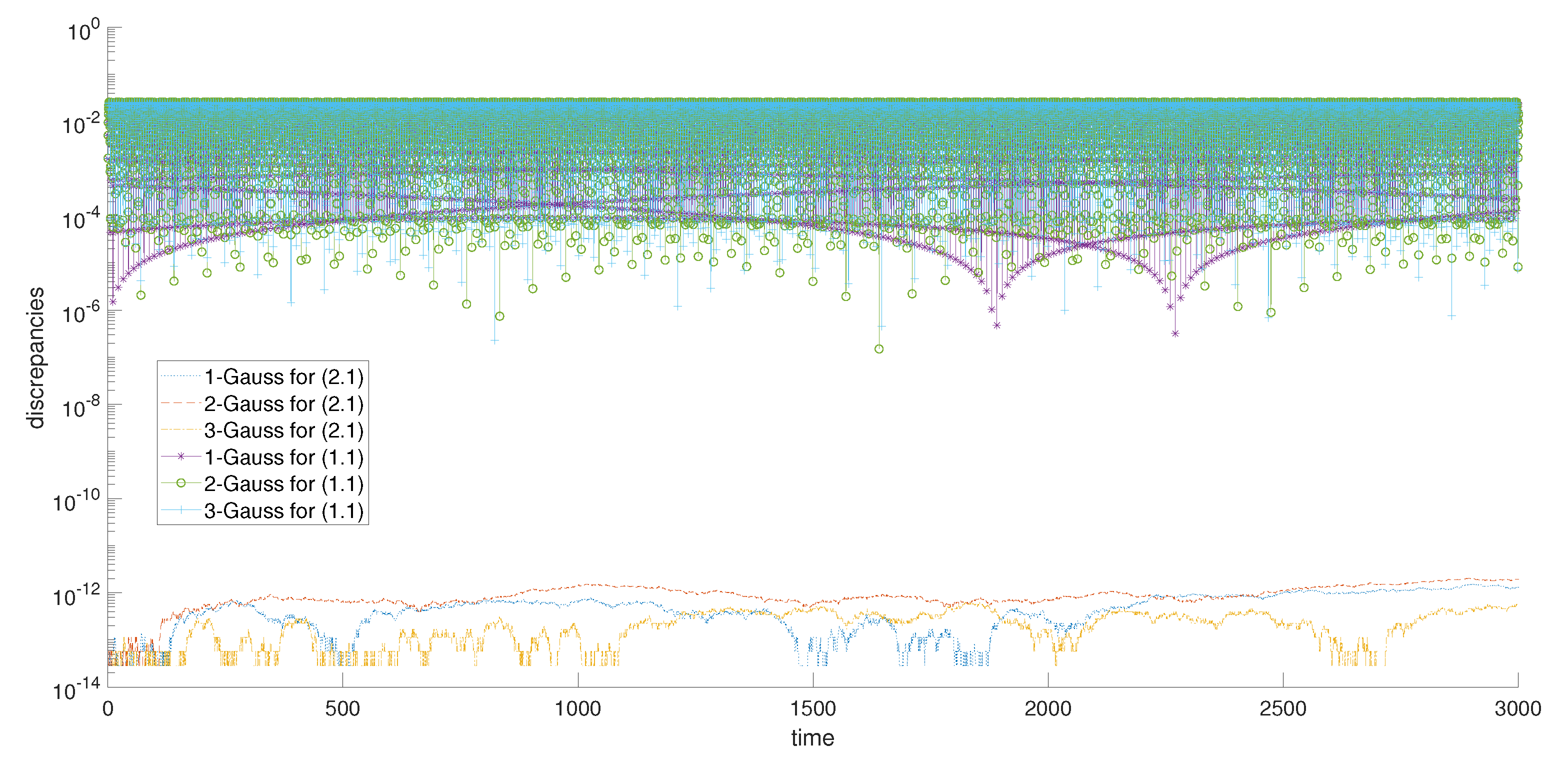
Figure 4.
The discrepancies of the discrete energy for Example 3.
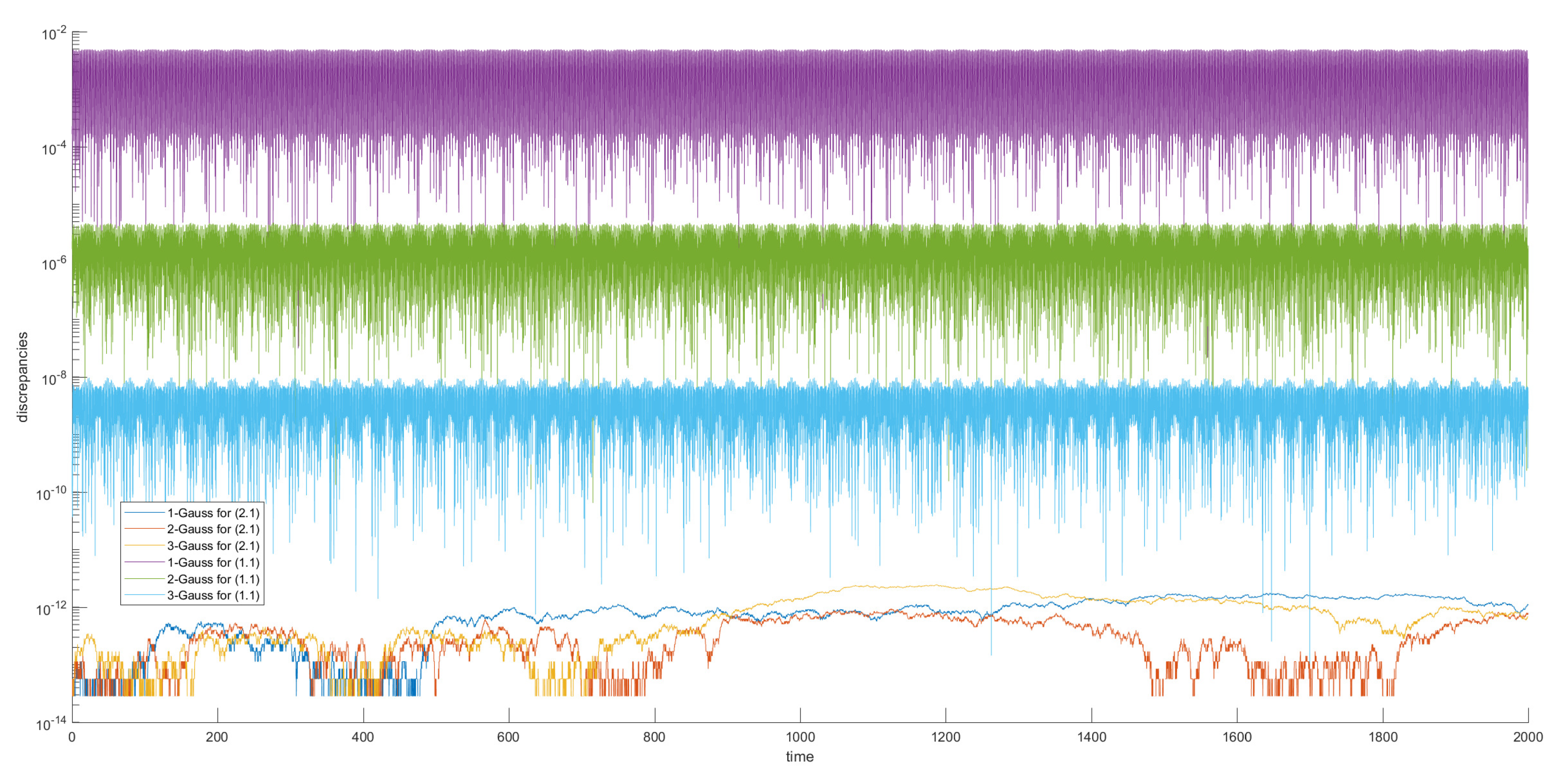
Figure 5.
The discrepancies of the discrete energy for Example 4.
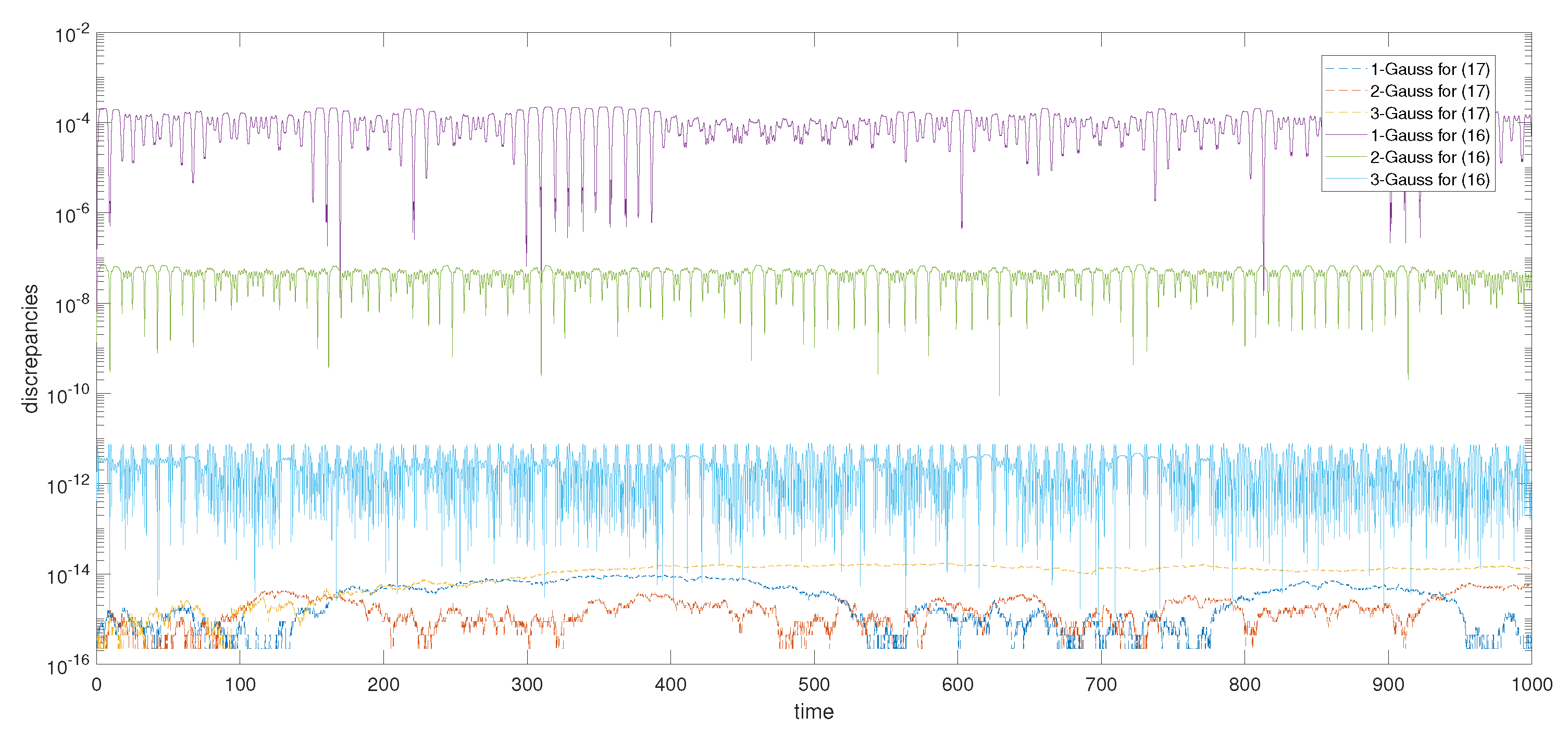
Figure 6.
The discrepancies of the discrete energy for Example 5.


Table 1.
The maximum errors at and convergence orders for Example 1.
| Method | h | p | q | r | |||
|---|---|---|---|---|---|---|---|
| e | Order | e | Order | e | Order | ||
| 1/10 | 7.06E−2 | - | 2.45E−2 | - | 7.49E−3 | - | |
| 1-Gauss | 1/20 | 1.18E−2 | 1.98 | 6.27E−3 | 1.97 | 1.89E−3 | 1.99 |
| 1/40 | 4.50E−3 | 1.98 | 1.58E−3 | 1.98 | 4.74E−4 | 1.99 | |
| 1/80 | 1.13E−3 | 1.99 | 3.95E−3 | 1.99 | 1.19E−4 | 1.99 | |
| 1/10 | 4.75E−4 | - | 1.26E−4 | - | 4.82E−5 | - | |
| 2-Gauss | 1/20 | 3.00E−5 | 3.99 | 8.09E−6 | 3.97 | 3.69E−6 | 3.71 |
| 1/40 | 1.88E−6 | 3.99 | 5.08E−7 | 3.98 | 2.30E−7 | 3.85 | |
| 1/80 | 1.18E−7 | 3.99 | 3.18E−8 | 3.99 | 1.45E−8 | 3.90 | |
| 1/10 | 3.10E−6 | - | 6.79E−7 | - | 4.41E−7 | - | |
| 3-Gauss | 1/20 | 5.22E−8 | 5.90 | 1.09E−8 | 5.96 | 9.96E−9 | 5.47 |
| 1/40 | 8.19E−10 | 5.94 | 1.73E−10 | 5.97 | 1.51E−10 | 5.76 | |
| 1/80 | 1.28E−11 | 5.96 | 2.71E−12 | 5.98 | 2.34E−12 | 5.84 | |
Table 2.
The maximum errors at and convergence orders for Example 2.
| Method | h | p | q | r | |||
|---|---|---|---|---|---|---|---|
| e | Order | e | Order | e | Order | ||
| 1/10 | 1.14E−4 | - | 1.27E−4 | - | 3.39E−5 | - | |
| 1-Gauss | 1/20 | 2.86E−5 | 2.00 | 3.18E−5 | 2.00 | 8.49E−6 | 2.00 |
| 1/40 | 7.14E−6 | 2.00 | 7.95E−6 | 2.00 | 2.12E−6 | 2.00 | |
| 1/80 | 1.79E−6 | 2.00 | 1.99E−6 | 2.00 | 5.31E−7 | 2.00 | |
| 1/10 | 3.45E−8 | - | 3.69E−8 | - | 1.03E−8 | - | |
| 2-Gauss | 1/20 | 2.16E−9 | 4.00 | 2.31E−9 | 4.00 | 6.46E−10 | 4.00 |
| 1/40 | 1.35E−10 | 4.00 | 1.44E−10 | 4.00 | 4.04E−11 | 4.00 | |
| 1/80 | 8.43E−12 | 4.00 | 9.02E−12 | 4.00 | 2.52E−12 | 4.00 | |
| 1/4 | 1.03E−9 | - | 1.12E−9 | - | 3.23E−10 | - | |
| 3-Gauss | 1/8 | 1.61E−11 | 6.00 | 1.75E−11 | 6.00 | 5.05E−12 | 6.00 |
| 1/16 | 2.54E−13 | 5.99 | 2.67E−13 | 6.02 | 7.90E−14 | 6.00 | |
| 1/32 | 5.55E−15 | 5.83 | 4.22E−15 | 6.01 | 1.94E−15 | 5.78 | |
Table 3.
The maximum errors at and convergence orders for Example 3.
| Method | h | p | q | r | |||
|---|---|---|---|---|---|---|---|
| e | Order | e | Order | e | Order | ||
| 1/10 | 1.41E−2 | - | 6.74E−3 | - | 9.77E−3 | - | |
| 1-Gauss | 1/20 | 3.55E−3 | 2.00 | 1.68E−3 | 2.00 | 2.43E−3 | 2.01 |
| 1/40 | 8.89E−4 | 2.00 | 4.21E−4 | 2.00 | 6.07E−4 | 2.00 | |
| 1/80 | 2.22E−4 | 2.00 | 1.05E−4 | 2.00 | 1.52E−4 | 2.00 | |
| 1/10 | 4.38E−6 | - | 2.03E−6 | - | 1.60E−6 | - | |
| 2-Gauss | 1/20 | 2.80E−7 | 3.97 | 1.27E−7 | 4.00 | 1.02E−7 | 3.98 |
| 1/40 | 1.76E−8 | 3.98 | 7.95E−9 | 4.00 | 6.43E−9 | 3.98 | |
| 1/80 | 1.10E−9 | 3.99 | 4.97E−10 | 4.00 | 4.02E−10 | 3.99 | |
| 1/4 | 2.03E−6 | - | 1.39E−6 | - | 8.64E−7 | - | |
| 3-Gauss | 1/8 | 2.73E−8 | 6.21 | 1.62E−8 | 6.42 | 1.20E−8 | 6.17 |
| 1/16 | 4.16E−10 | 6.13 | 2.48E−10 | 6.23 | 1.76E−10 | 6.13 | |
| 1/32 | 6.48E−12 | 6.09 | 3.83E−12 | 6.16 | 2.73E−12 | 6.09 | |
Table 4.
The maximum errors at and convergence orders for Example 4.
| Method | h | p | q | r | |||
|---|---|---|---|---|---|---|---|
| e | Order | e | Order | e | Order | ||
| 1/4 | 2.43E−3 | - | 5.03E−3 | - | 2.07E−4 | - | |
| 1-Gauss | 1/8 | 6.14E−4 | 1.99 | 1.28E−3 | 1.98 | 5.31E−5 | 1.96 |
| 1/16 | 1.54E−4 | 2.00 | 3.20E−4 | 2.00 | 1.34E−5 | 1.99 | |
| 1/32 | 3.85E−5 | 2.00 | 8.01E−5 | 2.00 | 3.35E−6 | 2.00 | |
| 1/4 | 6.64E−6 | - | 7.73E−6 | - | 1.11E−6 | - | |
| 2-Gauss | 1/8 | 4.15E−7 | 4.00 | 4.87E−7 | 3.99 | 6.90E−8 | 4.00 |
| 1/16 | 2.59E−8 | 4.00 | 3.05E−8 | 4.00 | 4.31E−9 | 4.00 | |
| 1/32 | 1.62E−9 | 4.00 | 1.91E−9 | 4.00 | 2.69E−10 | 4.00 | |
| 1/4 | 2.71E−9 | - | 1.25E−8 | - | 3.80E−10 | - | |
| 3-Gauss | 1/8 | 4.40E−11 | 5.95 | 1.96E−10 | 6.00 | 5.56E−12 | 6.09 |
| 1/12 | 3.88E−12 | 5.99 | 1.73E−11 | 6.00 | 4.86E−13 | 6.01 | |
| 1/16 | 6.90E−13 | 6.01 | 3.07E−12 | 6.00 | 8.93E−14 | 5.89 | |
Table 5.
The maximum errors at and convergence orders for Example 5.
| Method | h | p | q | r | |||
|---|---|---|---|---|---|---|---|
| e | Order | e | Order | e | Order | ||
| 1/4 | 3.28E−2 | - | 1.36E−2 | - | 8.82E−3 | - | |
| 1-Gauss | 1/8 | 7.86E−3 | 2.06 | 3.27E−3 | 2.05 | 2.04E−3 | 2.11 |
| 1/16 | 1.95E−3 | 2.01 | 8.11E−4 | 2.01 | 5.01E−4 | 2.03 | |
| 1/32 | 4.85E−4 | 2.00 | 2.02E−4 | 2.00 | 1.25E−4 | 2.01 | |
| 1/4 | 8.43E−5 | - | 4.76E−5 | - | 2.24E−5 | - | |
| 2-Gauss | 1/8 | 5.30E−6 | 3.99 | 2.99E−6 | 3.99 | 1.41E−6 | 3.99 |
| 1/16 | 3.32E−7 | 4.00 | 1.87E−7 | 4.00 | 8.84E−8 | 4.00 | |
| 1/32 | 2.08E−8 | 4.00 | 1.17E−8 | 4.00 | 5.53E−9 | 4.00 | |
| 1/4 | 1.14E−7 | - | 8.42E−8 | - | 4.12E−8 | - | |
| 3-Gauss | 1/8 | 1.80E−9 | 5.99 | 1.32E−9 | 6.00 | 6.48E−10 | 5.99 |
| 1/16 | 2.81E−11 | 6.00 | 2.07E−11 | 6.00 | 1.01E−11 | 6.00 | |
| 1/32 | 4.42E−13 | 5.99 | 3.26E−13 | 5.98 | 1.54E−13 | 6.04 | |
Publisher’s Note: MDPI stays neutral with regard to jurisdictional claims in published maps and institutional affiliations. |
© 2021 by the authors. Licensee MDPI, Basel, Switzerland. This article is an open access article distributed under the terms and conditions of the Creative Commons Attribution (CC BY) license (https://creativecommons.org/licenses/by/4.0/).
Share and Cite
MDPI and ACS Style
Tang, R.; Li, D. On Symmetrical Methods for Charged Particle Dynamics. Symmetry 2021, 13, 1626. https://doi.org/10.3390/sym13091626
AMA Style
Tang R, Li D. On Symmetrical Methods for Charged Particle Dynamics. Symmetry. 2021; 13(9):1626. https://doi.org/10.3390/sym13091626
Chicago/Turabian StyleTang, Renxuan, and Dongfang Li. 2021. "On Symmetrical Methods for Charged Particle Dynamics" Symmetry 13, no. 9: 1626. https://doi.org/10.3390/sym13091626
Note that from the first issue of 2016, this journal uses article numbers instead of page numbers. See further details here.