Influence of Wind Speed, Wind Direction and Turbulence Model for Bridge Hanger: A Case Study

Abstract

Wind field (e.g., wind speed and wind direction) has the characteristics of randomness, nonlinearity, and uncertainty, which can be critical and even destructive on a long-span bridge’s hangers, such as vortex shedding, galloping, and flutter. Nowadays, the finite element method is widely used for model calculation, such as in long-span bridges and high-rise buildings. In this study, the investigated bridge hanger model was established by COMSOL Multiphysics software, which can calculate fluid dynamics (CFD), solid mechanics, and fluid–solid coupling. Regarding the wind field of bridge hangers, the influence of CFD models, wind speed, and wind direction are investigated. Specifically, the bridge hanger structure has symmetrical characteristics, which can greatly reduce the calculation efficiency. Furthermore, the von Mises stress of bridge hangers is calculated based on fluid–solid coupling.

1. Introduction

In recent years, the structure of long-span bridges has been softer, and their crossing ability has shown a continuous increase due to the advance in design and construction technologies and the emergence of novel materials [1]. However, a long-span bridge does not work properly and is even destroyed under wind effects, which include vortex shedding, galloping, flutter, and so forth [2]. For example, vortex-induced vibrations may result in long-term fatigue damage, shortening the bridge life [3]. Galloping can lead to significant amplitude oscillation of the bridge [4]. Long-span bridges may be affected by dynamic instability phenomena, that is, flutter [5]. Therefore, it is important to analyze the impact of long-span bridges under wind fields (e.g., wind speed and wind direction), which can ensure a reliable wind-resistant design of a bridge [6,7,8,9,10,11,12].

In order to study the impact of long-span bridges under wind fields (e.g., wind speed and wind direction), computational fluid dynamics [13,14,15,16,17] has been proposed based on structural health monitoring (SHM) data. Regarding the influence of wind direction, Zhu et al. (2012) [18] found variations of aerodynamic coefficients with wind direction based on the results of wind tunnel tests. However, wind tunnel tests cannot be widely used in the study of a wind-induced structural response because these tests require a substantial amount of resources, where these tests are limited to a certain number of pressure taps, and some information about separation zones, recirculation, and so forth might get lost [19,20]. On the contrary, the numerical calculation method, that is, computational fluid dynamics model, can obtain the corresponding structural stress response by setting different wind speeds and wind directions based on the finite element method [21]. For example, Huang et al. [22] ran a 3D CFD model to examine scale effects on turbulent flow and sediment scour. Shirai et al. [23] studied the applicability of the two-dimensional Reynolds-averaged numerical simulation for predicting the flow around a self-oscillating bridge deck section. Thus, the computational fluid dynamics model allows for an accurate evaluation of the impact of long-span bridges under wind fields since it directly utilizes SHM data.

The main contributions of this work are threefold: (1) The bridge hanger model was established by COMSOL Multiphysics software, which can calculate computational fluid dynamics. (2) Regarding the bridge hanger, the influence of wind speed, wind direction, and turbulence model was investigated. The rest of the paper is organized as follows: In Section 2, the standard k-ε model, realizable k-ε model, standard k–ω model, and SST k-ω model of computational fluid dynamics are described. Section 3 introduces the results of the influence of wind speed, wind direction, and turbulence model. Finally, Section 4 ends with some conclusions drawn from this study.

2. Computational Fluid Dynamics

Generally, the computational fluid dynamics of a bridge are calculated based on the finite element method [24,25,26,27,28,29,30,31]. For an incompressible fluid, the continuity equation and momentum equation can be expressed as [32]

$$\frac{\partial U_i}{\partial x_i}=0$$

(1)

$$\begin{array}{c}{U}_j\frac{\partial U_i}{\partial x_j}=\frac{1}{\rho }\frac{\partial }{\partial x_j}(-P{\delta }_{ij}+2\upsilon S_{ij}+{\tau }_{ij})\\ S_{ij}=\frac{1}{2}\left(\frac{\partial U_i}{\partial x_j}+\frac{\partial U_j}{\partial x_i}\right)\end{array}$$

(2)

$${\tau }_{ij}={\upsilon }_t\left(\frac{\partial U_i}{\partial x_j}+\frac{\partial U_j}{\partial x_i}\right)-\frac{2}{3}k{\delta }_{ij}$$

(3)

where $\rho$ is the density of air, $\rho =1.293 {\mathrm{kg}/\mathrm{m}}^3$; $\upsilon$ is the kinematic viscosity, $\upsilon =17.9\times {10}^{-6} {\mathrm{m}}^2/\mathrm{s}$; $P$ is the pressure, Pa; $S_{ij}$ is the velocity strain rate tensor; ${\delta }_{ij}$ is the Kronecker delta; $U_i$ are the mean velocity components, m/s; and $k$ is the turbulent kinetic energy, m²/s².

Regarding the standard k-ε model, the transport equation of k can be expressed by [33]

$${\upsilon }_t=C_{\mu }\frac{k^2}{\epsilon }$$

(4)

$$\frac{\partial \rho k}{\partial t}+\frac{\partial \rho k{U}_i}{\partial x_i}=\frac{\partial }{\partial x_j}\left[\left(\upsilon +\frac{{\upsilon }_t}{{\sigma }_k}\right)\frac{\partial k}{\partial x_j}\right]+P_k-\rho \epsilon$$

(5)

$$\frac{\partial \rho \epsilon }{\partial t}+\frac{\partial \rho \epsilon U_i}{\partial x_i}=\frac{\partial }{\partial x_j}\left[\left(\upsilon +\frac{{\upsilon }_t}{{\sigma }_{\epsilon }}\right)\frac{\partial \epsilon }{\partial x_j}\right]+\frac{\epsilon }{k}\left(C_1{P}_k-C_2\rho \epsilon \right)$$

(6)

where $P_k$ is the production of turbulent kinetic energy, and $P_k={\upsilon }_t{S}^2$, $S=\sqrt{2S_{ij}{S}_{ij}}$, and other constants are $C_{\mu }=0.09$, ${\sigma }_{\epsilon }=1.3$, ${\sigma }_k=1.0$, $C_1=1.44$, and $C_2=1.92$.

Regarding the realizable k-ε model, the transport equation of k can be expressed by [34]

$$\frac{\partial \rho \epsilon }{\partial t}+\frac{\partial \rho \epsilon U_i}{\partial x_i}=\frac{\partial }{\partial x_j}\left[\left(\upsilon +\frac{{\upsilon }_t}{{\sigma }_{\epsilon }}\right)\frac{\partial \epsilon }{\partial x_j}\right]+\rho C_{\epsilon 1}S-\rho C_{\epsilon 2}\frac{{\epsilon }^2}{k+\sqrt{\epsilon \upsilon }}$$

(7)

where $\overline{{\Omega }_{ij}}$ is the mean rate-of-rotation tensor viewed in a rotating reference frame with the angular velocity ${\omega }_k$ and the constants are ${\sigma }_{\epsilon }=1.2$, $C_{\epsilon 2}=1.9$, $C_{\epsilon 1}=\max \left(0.43,\frac{k}{\epsilon }\sqrt{2S_{ij}{S}_{ij}}\right)$, $C_{\mu }=\frac{1}{4.04+\raisebox{1ex}{$A_{s}k{U}^{*}$}\!\left/ \!\raisebox{-1ex}{$\epsilon $}\right.}$, $A_s=\sqrt{6}\cos \theta$, $\theta =\frac{1}{3}\mathrm{co}{\mathrm{s}}^{-1}\sqrt{6}W$, $S^{*}=\sqrt{S_{ij}{S}_{ij}}$, $U^{*}=\sqrt{S_{ij}{S}_{ij}+{\Omega }^{*}{}_{ij}{\Omega }^{*}{}_{ij}}$, ${\Omega }^{*}{}_{ij}={\Omega }_{ij}-2{\epsilon }_{ijk}{\omega }_k$, and ${\Omega }_{ij}=\overline{{\Omega }_{ij}}-{\epsilon }_{ijk}{\omega }_k$.

Regarding the standard k-ω model, the transport equations of k and ω are defined by [35]

$${\upsilon }_{\omega t}=\frac{k}{\omega }$$

(8)

$$\frac{\partial k}{\partial t}+\frac{\partial k{U}_j}{\partial x_j}={\tau }_{ij}\frac{\partial U_j}{\partial x_j}-{\beta }^{*}k\omega \rho +\frac{\partial }{\partial x_j}\left[\left(\upsilon +{\upsilon }_{\omega t}{\sigma }_{k1}\right)\frac{\partial k}{\partial x_j}\right]$$

(9)

$$\frac{\partial \omega }{\partial t}+\frac{\partial \omega U_j}{\partial x_j}=\alpha \frac{\omega }{k}{\tau }_{ij}\frac{\partial U_j}{\partial x_j}-{\beta }_1{\omega }^2+\frac{\partial }{\partial x_j}\left[\left(\upsilon +{\upsilon }_{\omega t}{\sigma }_{\omega 1}\right)\frac{\partial \omega }{\partial x_j}\right]$$

(10)

where the constants are $\alpha =\frac{5}{9}$, ${\beta }_1=0.09$, ${\sigma }_{\omega 1}=0.5$, and ${\sigma }_{k1}=0.85$.

Regarding the SST k-ω model, the transport equations of k and ω are defined by [36,37]

$${\upsilon }_{\omega t}=\frac{a_{1}k}{\max \left(a_1\omega ,F_{2}S\right)}$$

(11)

$$\frac{\partial k}{\partial t}+\frac{\partial k{U}_j}{\partial x_j}=P_k-{\beta }^{*}k\omega +\frac{\partial }{\partial x_j}\left[\left(\upsilon +{\upsilon }_{\omega t}{\sigma }_{k2}\right)\frac{\partial k}{\partial x_j}\right]$$

(12)

$$\frac{\partial \omega }{\partial t}+\frac{\partial \omega U_j}{\partial x_j}=\alpha S^2-{\beta }_2{\omega }^2+\frac{\partial }{\partial x_j}\left[\left(\upsilon +{\upsilon }_{\omega t}{\sigma }_{\omega 2}\right)\frac{\partial \omega }{\partial x_j}\right]+2\left(1-F_1\right)\frac{{\sigma }_{\omega 2}}{\omega }\frac{\partial k}{\partial x_i}\frac{\partial \omega }{\partial x_i}$$

(13)

$$P_k=\min \left({\tau }_{ij}\frac{\partial U_i}{\partial x_j},10{\beta }^{*}k\omega \right)$$

(14)

$$F_1=\tanh \left\{{\left[\min \left(\max \left(\frac{\sqrt{k}}{{\beta }^{*}y\omega },\frac{500\upsilon }{y^2\omega }\right),\frac{4{\sigma }_{\omega 2}k}{C{D}_{k\omega }{y}^2}\right)\right]}^4\right\}$$

(15)

$$F_2=\tanh \left\{{\left[\max \left(\frac{2\sqrt{k}}{{\beta }^{*}y\omega },\frac{500\upsilon }{y^2\omega }\right)\right]}^2\right\}$$

(16)

$$C{D}_{k\omega }=\max \left(2\rho \frac{{\sigma }_{\omega 2}}{\omega }\frac{\partial k}{\partial x_i}\frac{\partial \omega }{\partial x_i},10^{-10}\right)$$

(17)

where the constants are ${\beta }_2=0.0828$, ${\sigma }_{\omega 2}=0.856$, ${\sigma }_{k2}=1$, and $a_1=0.31$.

3. Calculation and Analysis

Figure 1 shows the investigated bridge. Regarding the investigated bridge hangers, their diameter is 0.077 m, their modulus of elasticity is 1.9 × 10⁸ kpa, their bulk density is 7850 kN/m³, and their Poisson’s ratio is 0.3. Regarding the boundary conditions of the bridge hangers, they have a fixed constraint on the upper and lower.

COMSOL Multiphysics is a general finite element software that can be used to calculate fluid dynamics, solid mechanics, multifield coupling, and so forth [38]. Regarding the finite element model, the left boundary is the wind speed inlet, the right boundary is the outlet, and the upper and lower boundaries are slip boundaries, which are the same boundary conditions with a wind tunnel test. Regarding the bridge section, there are 9994 domain elements and 334 boundary elements, and the mesh is encrypted at the boundary. Regarding the finite element model, it has the four slip boundaries, the wind speed inlet, and the wind speed outlet, which can be seen in Figure 2a. Finally, the finite element model is divided into 35,377,709 units based on the finite volume method to solve the fluid governing equations, which can be seen in Figure 2b.

3.1. Influence of CFD Models

In this case study, the wind speed is 12 m/s and the wind direction is 90 degree. The changes in a bridge hanger’s wind field at different CFD models are calculated, which can be seen as Figure 3. The calculation result of the SST k-ω model is different from that of the standard k-ε model, realizable k-ε model, and standard k-ω model, such as the wake flow characteristics of a hanger. Regarding the calculation result of the standard k-ε model, realizable k-ε model, and standard k-ω model, their wind field is the same. Therefore, the standard k-ε model is selected to calculate the turbulence equation.

3.2. Influence of Wind Speed

In this case study, we assume the wind direction is 0 degree and the wind speed is adjustable. The changes in the bridge hangers’ stress at different wind speeds are calculated based on the k–ε model and dynamic equations, which can be seen in Figure 4. When the wind speed increases from 3 to 12 m/s, the von Mises stress of the bridge hangers is nonlinearly increasing.

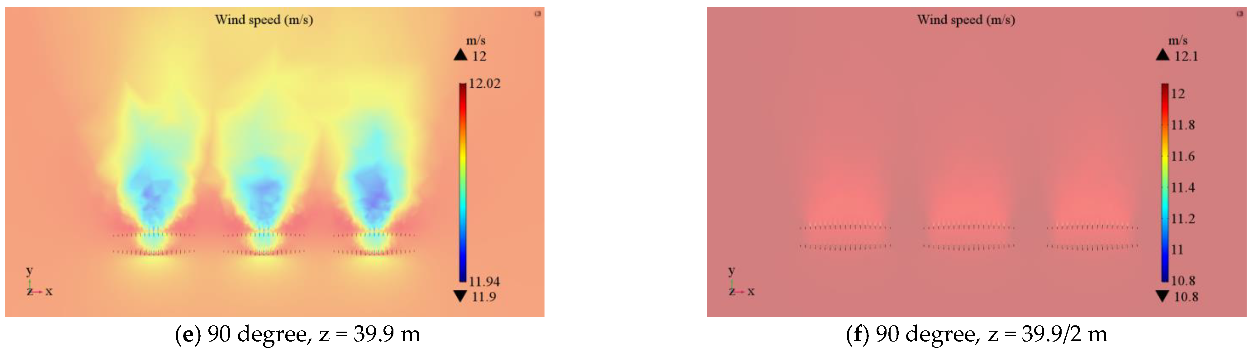
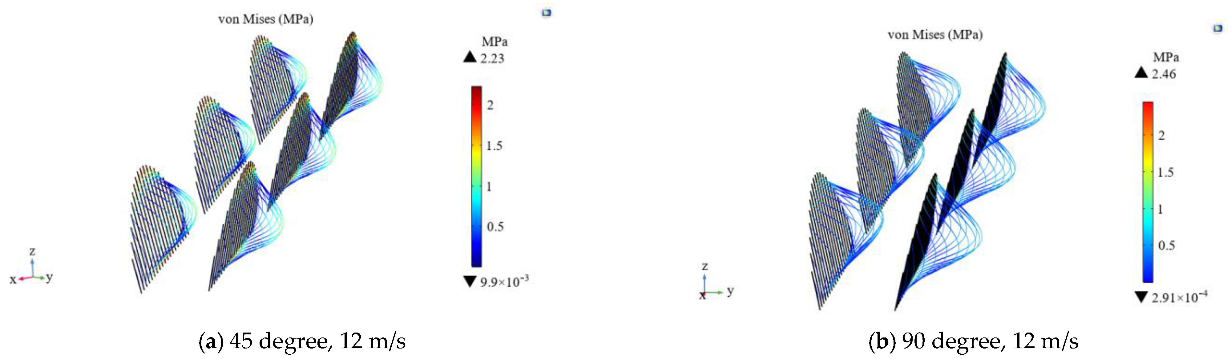
3.3. Influence of Wind Direction

In this case study, the wind speed is 12 m/s and the wind direction is adjustable. The changes in the bridge hangers’ wind field at different wind directions are calculated based on the k–ε model and dynamic equations, which can be seen in Figure 5. On the one hand, the wind field is different at different heights with the same wind speed. On the other hand, when the wind direction increases from 0 to 90 degrees, the wind speed field changes too.

The changes in the bridge hangers’ stress at different wind directions are calculated based on the k–ε model and dynamic equations, which can be seen in Figure 4d and Figure 6.

4. Discussion and Conclusions

This case analyzes the finite element model of investigated bridge hangers through COMSOL Multiphysics software. The influences of CFD models, wind speed, and wind direction on the bridge hangers are investigated through case studies, and the von Mises stress of the bridge hangers is calculated based on fluid–solid coupling. The main conclusions drawn from this study are summarized as follows:

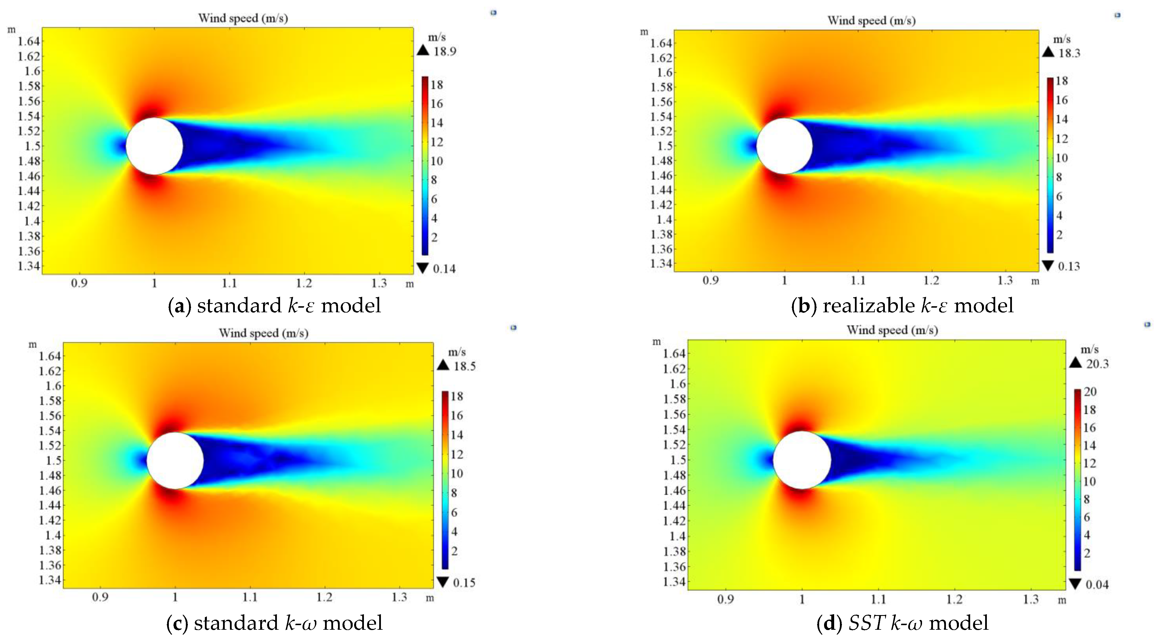
• The calculation result of the SST k-ω model is different from that of the standard k-ε model, realizable k-ε model, and standard k-ω model, such as the wake flow characteristics of a hanger. Therefore, we will use the standard k-ε model to calculate the von Mises stress time history curve of bridge hangers and then assess the fatigue life of bridge hangers in a future work.
• The larger is the wind speed, the larger is the effect on the wind field and stress for the investigated bridge hangers. For example, when the wind speed increases from 3 to 12 m/s, the stress of the bridge hangers nonlinearly increases. Therefore, the influence of the bridge hangers should be a concern under a strong wind speed during the operation.
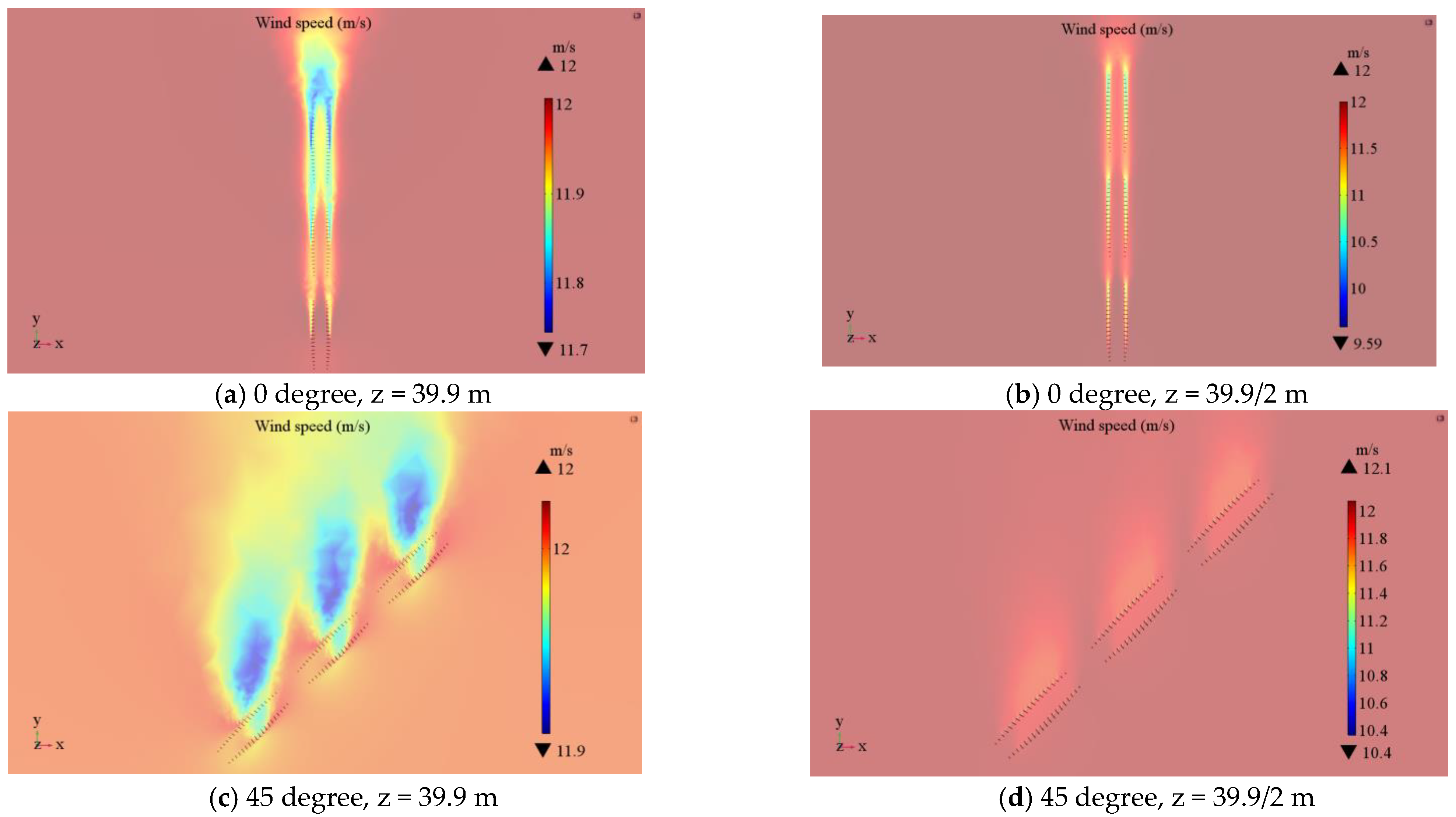
• Regarding the different wind directions with the same wind speed, the influence of the bridge hangers is also different. For example, when the wind direction increases from 0 to 90 degrees, the fatigue life of the bridge hangers decreases. Therefore, the influence of wind direction on the investigated bridge hangers cannot be ignored.

References

- Xu, S.Q.; Ma, R.J.; Wang, D.; Chen, A.; Tian, H. Prediction analysis of vortex-induced vibration of long-span suspension bridge based on monitoring data. J. Wind Eng. Ind. Aerodyn. 2019, 191, 312–324. [Google Scholar] [CrossRef]
- Shum, K.M.; Xu, Y.L.; Guo, W.H. Wind-induced vibration control of long span cable-stayed bridges using multiple pressurized tuned liquid column dampers. J. Wind Eng. Ind. Aerodyn. 2008, 96, 166–192. [Google Scholar] [CrossRef]
- Li, S.; Laima, S.; Li, H. Data-driven modeling of vortex-induced vibration of a long-span suspension bridge using decision tree learning and support vector regression. J. Wind Eng. Ind. Aerodyn. 2018, 172, 196–211. [Google Scholar] [CrossRef]
- Li, S.L.; An, Y.H.; Wang, C.Q.; Wang, D.W. Experimental and numerical studies on galloping of the flat-topped main cables for the long span suspension bridge during construction. J. Wind Eng. Ind. Aerodyn. 2017, 163, 24–32. [Google Scholar] [CrossRef]
- Casalotti, A.; Arena, A.; Lacarbonara, W. Mitigation of post-flutter oscillations in suspension bridges by hysteretic tuned mass dampers. Eng. Struct. 2014, 69, 62–71. [Google Scholar] [CrossRef]
- Ding, Y.; Dong, J.; Yang, T.; Zhou, S.; Wei, Y. Failure Evaluation of Bridge Deck Based on Parallel Connection Bayesian Network: Analytical Model. Materials 2021, 14, 1411. [Google Scholar] [CrossRef] [PubMed]
- Ni, Y.Q.; Xia, Y.; Liao, W.Y.; Ko, J.M. Technology innovation in developing the structural health monitoring system for guangzhou new tv tower. Struct. Control Health Monit. 2009, 16, 73–98. [Google Scholar] [CrossRef]
- Lin, L.; Chen, K.; Xia, D.; Wang, H.; Hu, H.; He, F. Analysis on the wind characteristics under typhoon climate at the southeast coast of china. J. Wind Eng. Ind. Aerodyn. 2018, 182, 37–48. [Google Scholar] [CrossRef]
- Wang, H.; Li, A.; Niu, J.; Zong, Z.; Li, J. Long-term monitoring of wind characteristics at sutong bridge site. J. Wind Eng. Ind. Aerodyn. 2013, 115, 39–47. [Google Scholar] [CrossRef]
- Xu, Y.L. Making good use of structural health monitoring systems of long-span cable-supported bridges. J. Civ. Struct. Health Monit. 2018, 8, 477–497. [Google Scholar] [CrossRef]
- Koo, K.Y.; Brownjohn, J.M.W.; List, D.I.; Cole, R. Structural health monitoring of the Tamar suspension bridge. Struct. Control Health Monit. 2013, 20, 609–625. [Google Scholar] [CrossRef] [Green Version]
- Ding, Y.; Zhou, G.; Li, A.; Deng, Y. Statistical characteristics of sustained wind environment for a long-span bridge based on long-term field measurement data. Wind Struct. 2013, 17, 43–68. [Google Scholar] [CrossRef]
- Saha, U.K.; Thotla, S.; Maity, D. Optimum design configuration of savonius rotor through wind tunnel experiments. J. Wind Eng. Ind. Aerodyn. 2008, 96, 1359–1375. [Google Scholar] [CrossRef]
- Zajaczkowski, F.J.; Haupt, S.E.; Schmehl, K.J.; Jweia, J.; Model, W.F. A preliminary study of assimilating numerical weather prediction data into computational fluid dynamics models for wind prediction. J. Wind Eng. Ind. Aerodyn. 2011, 99, 320–329. [Google Scholar] [CrossRef]
- Jeong, W.M.; Liu, S.N.; Jakobsen, J.B.; Ong, M.C. Unsteady RANS simulations of flow around a twin-box bridge girder cross section. Energies 2019, 12, 2670. [Google Scholar] [CrossRef] [Green Version]
- Matsumoto, M.; Shijo, R.; Eguchi, A.; Hikida, T.; Mizuno, K. On the flutter characteristics of separated two box girders. Wind Struct. Int. J. 2004, 7, 281–291. [Google Scholar] [CrossRef]
- Hu, C.; Zhou, Z.; Jiang, B. Effects of types of bridge decks on competitive relationships between aerostatic and flutter stability for a super long cable-stayed bridge. Wind Struct. 2019, 28, 255–270. [Google Scholar]
- Zhu, L.D.; Li, L.; Xu, Y.L.; Zhu, Q. Wind tunnel investigations of aerodynamic coefficients of road vehicles on bridge deck. J. Fluids Struct. 2012, 30, 35–50. [Google Scholar] [CrossRef]
- Montoya, M.C.; Nieto, F.; Hernández, S.; Kusano, I.; Jurado, J.Á. Cfd-based aeroelastic characterization of streamlined bridge deck cross-sections subject to shape modifications using surrogate models. J. Wind Eng. Ind. Aerodyn. 2018, 177, 405–428. [Google Scholar] [CrossRef]
- Thordal, M.S.; Bennetsen, J.C.; Koss, H.H.H. Review for practical application of cfd for the determination of wind load on high-rise buildings. J. Wind Eng. Ind. Aerodyn. 2019, 186, 155–168. [Google Scholar] [CrossRef]
- Scappaticci, L.; Castellani, F.; Astolfi, D.; Garinei, A. Diagnosis of vortex induced vibration of a gravity damper. Diagnostyka 2018, 19, 31–39. [Google Scholar] [CrossRef]
- Huang, W.; Yang, Q.; Hong, X. Cfd modeling of scale effects on turbulence flow and scour around bridge piers. Comput. Fluids 2009, 38, 1050–1058. [Google Scholar] [CrossRef]
- Shirai, S.; Ueda, T. Aerodynamic simulation by cfd on flat box girder of super-long-span suspension bridge. J. Wind Eng. Ind. Aerodyn. 2003, 91, 279–290. [Google Scholar] [CrossRef]
- Khalilzadeh, A.; Ge, H.; Ng, H.D. Effect of turbulence modeling schemes on wind-driven rain deposition on a mid-rise building: Cfd modeling and validation. J. Wind Eng. Ind. Aerodyn. 2019, 184, 362–377. [Google Scholar] [CrossRef]
- Haque, S.M.E.; Rasul, M.G.; Khan, M.M.K.; Deev, A.V.; Subaschandar, N. Influence of the inlet velocity profiles on the prediction of velocity distribution inside an electrostatic precipitator. Exp. Therm. Fluid Sci. 2009, 33, 322–328. [Google Scholar] [CrossRef]
- Sun, D.; Owen, J.S.; Wright, N.G. Application of the k–ω turbulence model for a wind-induced vibration study of 2d bluff bodies. J. Wind Eng. Ind. Aerodyn. 2009, 97, 77–87. [Google Scholar] [CrossRef]
- Xu, G.; Cai, C.S. Numerical investigation of the lateral restraining stiffness effect on the bridge deck-wave interaction under stokes waves. Eng. Struct. 2017, 130, 112–123. [Google Scholar] [CrossRef] [Green Version]
- De, M.S.; Patruno, L.; Ubertini, F.; Vairo, G. Indicial functions and flutter derivatives: A generalized approach to the motion-related wind loads. J. Fluids Struct. 2013, 42, 466–487. [Google Scholar]
- Glück, M.; Breuer, M.; Durst, F.; Halfmann, A.; Rank, E. Computation of wind-induced vibrations of flexible shells and membranous structures. J. Fluids Struct. 2003, 17, 739–765. [Google Scholar] [CrossRef]
- Santo, G.; Peeters, M.; Van Paepegem, W.; Degroote, J. Dynamic load and stress analysis of a large horizontal axis wind turbine using full scale fluid-structure interaction simulation. Renew. Energy 2019, 140, 212–226. [Google Scholar] [CrossRef]
- Wu, Y.L.; Qi, L.J.; Zhang, H.; Musiu, E.; Yang, Z.P.; Wang, P. Design of UAV downwash airflow field detection system based on strain effect principle. Sensors 2019, 19, 2630. [Google Scholar] [CrossRef] [Green Version]
- Qi, Y.H.; Ishihara, T. Numerical study of turbulent flow fields around of a row of trees and an isolated building by using modified k-ε model and les model. J. Wind Eng. Ind. Aerodyn. 2018, 177, 293–305. [Google Scholar] [CrossRef]
- Nakajima, K.; Ooka, R.; Kikumoto, H. Evaluation of k-ε reynolds stress modeling in an idealized urban canyon using les. J. Wind Eng. Ind. Aerodyn. 2018, 175, 213–228. [Google Scholar] [CrossRef]
- Lateb, M.; Masson, C.; Stathopoulos, T.; Bédard, C. Comparison of various types of k–ε models for pollutant emissions around a two-building configuration. J. Wind Eng. Ind. Aerodyn. 2013, 115, 9–21. [Google Scholar] [CrossRef] [Green Version]
- Wilcox, D.C. Reassessment of the scale-determining equation for advanced turbulence models. AIAA J. 1988, 26, 1299–1310. [Google Scholar] [CrossRef]
- Menter, F.R. Two-equation eddy-viscosity turbulence models for engineering applications. AIAA J. 1994, 32, 1598–1605. [Google Scholar] [CrossRef] [Green Version]
- Menter, F.R. Zonal two equation k-ω turbulence models for aerodynamic flows. AIAA J. 1993, 6, 2893–2906. [Google Scholar]
- Ding, Y.; Yang, T.L.; Liu, H.; Han, Z.; Zhou, S.X.; Wang, Z.P.; She, A.M.; Wei, Y.-Q.; Dong, J.L. Experimental study and simulation calculation of the chloride resistance of concrete under multiple factors. Appl. Sci. 2021, 11, 5322. [Google Scholar] [CrossRef]
Publisher’s Note: MDPI stays neutral with regard to jurisdictional claims in published maps and institutional affiliations. |
© 2021 by the authors. Licensee MDPI, Basel, Switzerland. This article is an open access article distributed under the terms and conditions of the Creative Commons Attribution (CC BY) license (https://creativecommons.org/licenses/by/4.0/).
Share and Cite
Ding, Y.; Zhou, S.-X.; Wei, Y.-Q.; Yang, T.-L.; Dong, J.-L. Influence of Wind Speed, Wind Direction and Turbulence Model for Bridge Hanger: A Case Study. Symmetry 2021, 13, 1633. https://doi.org/10.3390/sym13091633
Ding Y, Zhou S-X, Wei Y-Q, Yang T-L, Dong J-L. Influence of Wind Speed, Wind Direction and Turbulence Model for Bridge Hanger: A Case Study. Symmetry. 2021; 13(9):1633. https://doi.org/10.3390/sym13091633
Chicago/Turabian StyleDing, Yang, Shuang-Xi Zhou, Yong-Qi Wei, Tong-Lin Yang, and Jing-Liang Dong. 2021. "Influence of Wind Speed, Wind Direction and Turbulence Model for Bridge Hanger: A Case Study" Symmetry 13, no. 9: 1633. https://doi.org/10.3390/sym13091633