1. Introduction
The spin glass model originates from condensed matter physics, where it was applied to physical systems in which magnetic atoms are randomly distributed in a non-magnetic host and induce ferromagnetic and antiferromagnetic interactions between neighboring magnetic moments. The physical system is mathematically modeled by a weighted graph where each vertex corresponds to a spin and each edge represents the interaction between spins with positive and negative signs [
1,
2]. In the Ising spin model, the spin is a binary variable that takes the value ± 1 [
3,
4]. The Ising problem is to find a binary spin configuration that minimizes the total energy function (the number of frustrated edges) for a given set of edges. A variety of combinatorial optimization problems, such as sequencing and ordering problems, resource allocation problems, and clustering problems [
5,
6], can be mapped to the Ising problem [
7].
To solve the Ising problem using a brute force combination approach, we need to check 2
n possibilities, where
n is the total number of spins. The branch and bound method, which based on a tree search algorithm, is commonly used to find the exact ground state without an exhaustive search [
8]. However, this method still requires a lot of CPU time and memory and is only applicable to instances with a small number of spins. The potential applications of the Ising model to optimization problems have motivated the development of heuristic algorithms for finding high-quality solutions for instances with a large number of spins [
9,
10]. Although heuristic algorithms generally do not guarantee an optimal solution, they can yield good time-to-solution in practice.
Simulated annealing (SA), one of the most common heuristic algorithms, mimics the physical process of annealing, where a material is slowly cooled to obtain the lowest energy state [
11,
12,
13]. Its algorithm is based on Monte Carlo simulation. Starting with an initial spin configuration, a new candidate configuration is selected in each iteration of the simulation. If the total energy decreases for the new candidate, that candidate is accepted and the iterative process continues. Otherwise, it is accepted with a probability given by the Boltzmann factor, which decreases with temperature. This random acceptance allows the algorithm to escape local minima. The system eventually cools into the global minimum in the spin configuration space.
The growth of data size in Ising problems has spurred interest in physical hardware systems that directly minimize the energy function [
14,
15,
16,
17,
18,
19,
20,
21]. Such systems are called Ising machines. An example of an Ising machine is the quantum annealing machine from D-Wave Systems, which was implemented using superconducting qubits [
22,
23]. The machine operates at a cryogenic temperature. The connectivity between qubits is limited to rather simple structures. Quantum adiabatic optimization inspired a new heuristic algorithm for the Ising problem, called simulated bifurcation, which simulates adiabatic evolution of classical nonlinear oscillators that exhibit bifurcation [
24,
25].
We recently developed a heuristic algorithm for the Ising problem in which the Ising spin system is replaced by a coupled oscillator system, which is possible owing to the equivalence of their equations of motion [
26]. We obtained exact ground states for problems with a small number of spins by simply calculating the lowest mode of the coupled oscillators (i.e., the lowest eigenvalue and eigenvector of the matrix representing the equations of motion). We also developed an error correction algorithm that modifies the coupling strength depending on the amplitude of individual oscillators. This heuristic algorithm is a kind of annealing process since the energy landscape in the dipole configuration space is optimized in such a way that the correct configuration is equivalent to the lowest eigenmode. Based on this concept, we proposed an Ising machine composed of plasmon particles with dipole–dipole interaction, whose strength can be modified by a phase-change material inserted between neighboring particles [
27].
In the present paper, we reconsider the coupled oscillator solver (COS) described above from the following viewpoints: (1) the lowest mode of the coupled oscillators may not always provide a minimally frustrated spin configuration (exact ground state) for large-sized Ising problems; and (2) it is desirable to replace the time-consuming error correction algorithm with a better algorithm inspired by an analysis of good candidate solutions (i.e., the lowest eigenmodes). We apply the COS to two-dimensional N × N oscillators for N values of up to 50. A map of the oscillation amplitudes (eigenvector components) of lower-frequency eigenmodes enables us to visualize unfrustrated clusters. We found that frustration tends to localize at the boundary between clusters due to the symmetric and asymmetric nature of the eigenmodes. This allows us to reduce frustration simply by flipping the sign of the amplitude of highly frustrated oscillators.
2. Coupled Oscillator Solver Applied to Ising Spin Problems
Here, we consider a square lattice (N × N) Ising spin glass problem without an external magnetic field. The spin configuration that minimizes the Ising energy is given by
where
si denotes the
ith spin with a value of 1 or −1, and
Jij is the coupling coefficient between the
ith and
jth spins having both positive (+
J; ferromagnetic coupling) and negative (−
J; antiferromagnetic coupling) values. In this study, only four nearest neighbor couplings are taken into account. For a given spin configuration, when
Jijsisj > 0, the coupling
Jij is satisfied, otherwise it is frustrated. Minimizing the Ising energy is equivalent to maximizing the number of satisfied couplings.
We start with an instance of 10 × 10 (N = 10) spins with 200 couplings. Problems were generated by randomly assigning ferromagnetic and antiferromagnetic couplings with a number ratio of 1:1.
Figure 1a shows the distribution of frustrated couplings (bold lines) for the exact ground state provided by a public domain [
28], where an algorithm in [
29] is used. In this algorithm, the original graph underlying the Ising problem is transformed into a dual graph, and minimum weight perfect matching is calculated. For the backward transformation, the matching leads to an Eulerian subgraph, the weight of which is also minimized. Owing to the one-to-one correspondence between the Eulerian subgraphs (cycles) and cuts in the original graph, the optimum Eulerian subgraphs provide the exact ground state for the Ising problem. The red circles and blue diamonds represent up-spin and down-spin states, respectively. The number of satisfied couplings of the exact ground state was found to be
nE = 166.
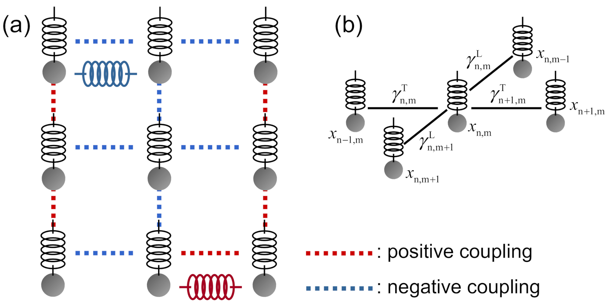
To solve the problem, we converted it to a classical coupled oscillator model by replacing the ferromagnetic and antiferromagnetic couplings with positive and negative couplings, respectively, between neighboring oscillators, as illustrated in
Figure 2a. A normal attractive spring connecting neighboring masses gives rise to a positive interaction, and the masses tend to move in the same direction at lower frequency. A negative interaction is implemented by a repulsive spring (which does not exist in reality) to allow the masses to move in opposite directions. Due to the mathematical similarity between the inter-spin and inter-oscillator interactions, we anticipate that the sign of the oscillator amplitude for the lowest mode is the same or close to the spin configuration for the exact ground state for the original Ising problem.
The equation of motion for the masses on the square lattice is given by
where
xn,m is the displacement of a mass at the (n, m) lattice site and α is the square root of the spring constant divided by the mass, which represents the strength of the coupling between neighboring oscillators. Here,
γn,m is +1 for positive interaction and −1 for negative interaction, and “T” and “L” indicate the transverse and longitudinal directions, respectively. The definition of the superscripts and subscripts associated with
γ is given in
Figure 2b. The eigenmodes of the collective motion of oscillators can be calculated by substituting
xn,m =
un,m exp(−i
ωt) into Equation (2) to obtain
By assuming a periodic boundary condition for
γn,m, Equation (3) for the N × N system can be reduced to the problem of calculating the eigenvalue (frequency)
ω and eigenvector (amplitude)
un,m for N
2 elements.
Figure 1b shows a map of the oscillation amplitude
un,m of the lowest four eigenmodes (eigenmode number
k = 1 to 4) for the original Ising problem. The circles and diamonds respectively represent positive and negative signs of
un,m. The distribution of
un,m is not localized; it covers the entire system. If two neighboring oscillators connected by positive (negative) coupling move in opposite directions (the same direction), they are considered to be frustrated, analogous to the Ising spin model. Frustrated couplings are indicated by bold lines in
Figure 1b. For instance, the two oscillators enclosed by the dotted ellipse in
Figure 1b move in opposite directions, as indicated by
un,m < 0 for the upper oscillator and
un,m > 0 for the lower oscillator. Since the coupling is positive, which is evident by the frustrated coupling (connected by the bold line) of the two corresponding spins with opposite signs shown in
Figure 1a, the oscillators are also frustrated for the eigenmode with
k = 1. A lower frequency (eigenmode number) typically yields a smaller number of frustrated couplings (but not strictly, as demonstrated in
Figure 1c).
The number of satisfied couplings
nCO as a function of eigenmode number
k is plotted in
Figure 1c.
nCO is maximized at the second lowest mode (
k = 2) and tends to decrease with
k. The maximum
nCO (
nCOmax) is 164, which corresponds to 98.7% of
nE (=166).
Figure 1d–f show the results for another instance of the system. Also in this case, the distribution of the amplitude
un,m is delocalized.
nCO is a maximum at
k = 3, for which
nCOmax is 166 or 97.6% of
nE (=170).
Table 1 summarizes the values of
k that maximize
nCO and
nCOmax/
nE for nine different instances. For all cases,
nCO is a maximum at
k ≤ 3 and
nCOmax/
nE is larger than 94.1%.
3. Eigenmode Mapping to Visualize Frustration Localization
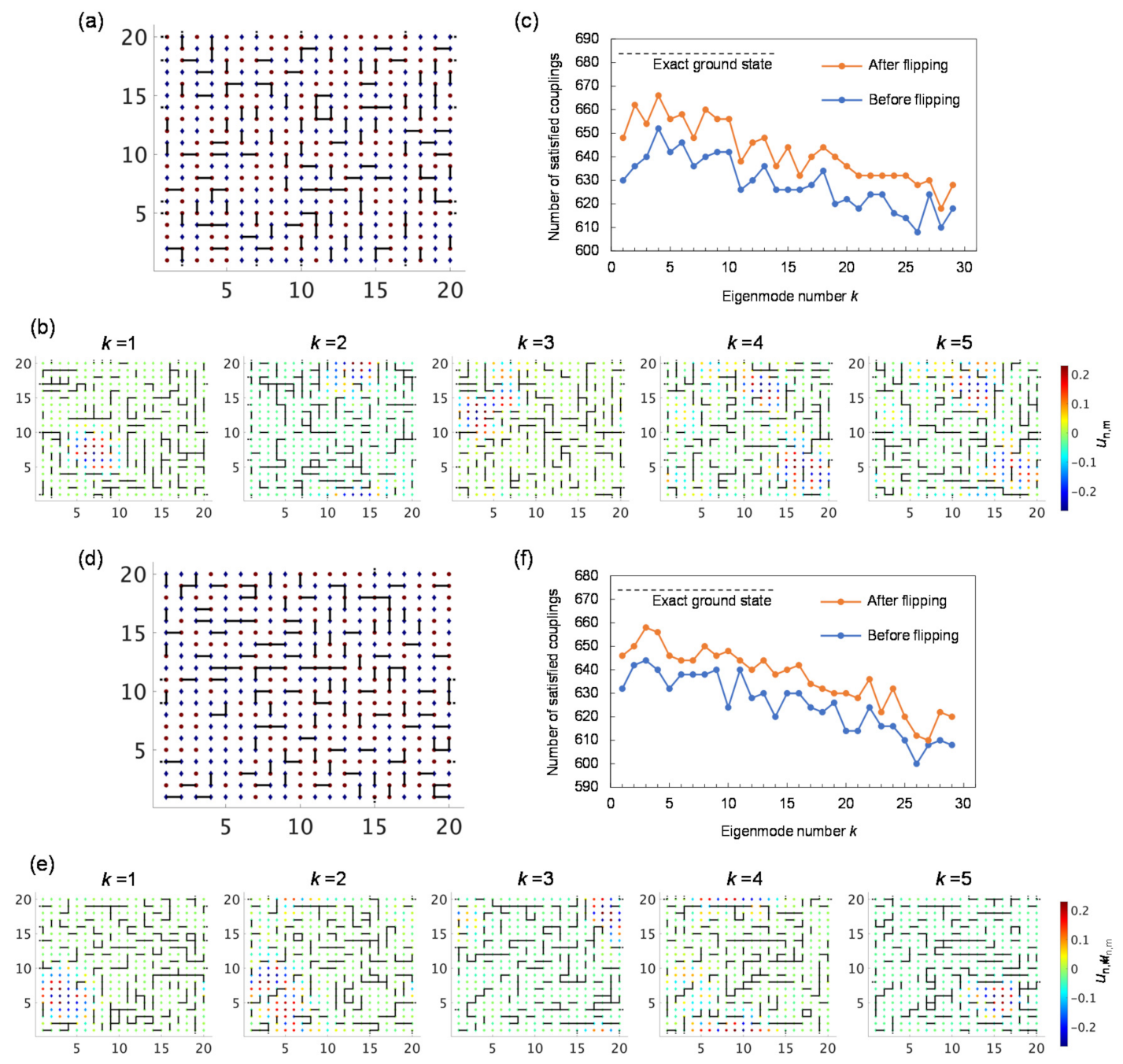
Next, we increase the problem size to 20 × 20 (N = 20). The distribution of frustrated couplings for the exact ground state is shown in
Figure 3a. The problem was converted to the coupled oscillator model and the eigenvalues and eigenvectors were calculated.
Figure 3b shows a map of the oscillation amplitude and frustrated couplings for eigenmode numbers of
k = 1 to 5.
Figure 3d,e show the results for another instance. In contrast to the smaller problem with N = 10, the collective oscillation is spatially localized and clusters form depending on
k. It is reasonable that the distribution of the signs of
un,m in each cluster is in complete agreement with that of the spin configuration in the exact ground state. The formation of such unfrustrated clusters can specify the region where frustration occurs with high probability since the oscillator system lowers the eigenfrequency by reducing the amplitude of the oscillators around which frustrated couplings are localized. In particular, for lower eigenmodes, the unfrustrated clusters tend to extend as widely as possible, making frustrated couplings as localized as possible at the boundary between unfrustrated clusters. In
Figure 3b, there are many oscillators around which three of the four couplings are frustrated. For these oscillators, the number of frustrated couplings can be reduced from three to one by flipping the sign of the amplitude.
Figure 3c shows
nCO before and after the flipping process as a function of
k, demonstrating the effectiveness of flipping in reducing frustration.
nCOmax is obtained for
k = 4 after flipping and
nCOmax/
nE reaches 97.7%. For the other problem (
Figure 3f),
nCOmax/
nE is a maximum (97.6%) at
k = 3.
Table 2 shows the results for nine instances, including the value of
k required to maximize
nCO and
nCOmax/
nE before and after flipping, to evaluate the effectiveness of flipping. For all cases,
nCO is a maximum at
k ≤ 8 and
nCOmax/
nE after flipping is larger than 96.7%. The eigenmode calculation is useful for visualizing unfrustrated clusters to find a fairly good solution, in which frustrated couplings are strongly localized around specific oscillators. The solution is effectively improved by flipping the sign of the amplitude to reduce frustration. It should be mentioned that it is relatively less probable for the lowest eigenmode (
k = 1) to provide the highest
nCOmax/
nE. This might be due to the fact that the amplitude distribution has more nodes between unfrustrated clusters for a few higher eigenmodes and the frustration is more localized in the vicinity of the nodes. To summarize, what the COS does before flipping is to find the eigenmode consisting of clusters without nodes (locally symmetric), and simultaneously localizing nodes at the cluster boundaries (globally asymmetric).
4. Application to Larger Problems and Benchmark
To demonstrate the performance of the algorithm, we applied it to larger problems.
Table 3 and
Table 4 summarizes the value of
k required to maximize
nCO and
nCOmax/
nE before and after flipping for nine instances of problems with N = 30 and 40, respectively. It is confirmed that lower eigenmodes provide good candidates and that the flipping process effectively improves the candidates. For N = 30,
nCO is a maximum at
k ≤ 9 and
nCOmax/
nE after flipping is larger than 96.6%. For N = 40,
nCO is a maximum at
k ≤ 13 and
nCOmax/
nE after flipping is larger than 96.7%. Overall, for N = 10 to 40, the best solution can be found by checking the lowest ~N/2 candidates.
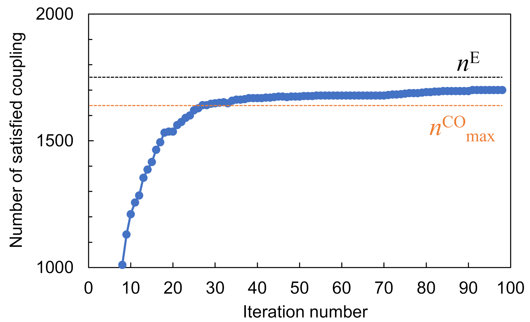
As a benchmark study, the computation time is compared between the COS and a standard SA algorithm for ten instances of problems with N = 50. All trials were performed on a MacBook Pro with a 2.6-GHz Intel
® Core i7 processor (6 cores) and 16 GB of RAM. The COS generated
nCOmax in 2.74 s, including the time required for the flipping process.
Figure 4 shows the evolution of the number of satisfied couplings with iteration number in SA for a given problem.
nCOmax and
nE are also indicated. After 27 iterations, SA provides a better solution than that provided by the COS. The computation time required to reach
nCOmax (27 iterations) was 8.63 s.
Table 5 compares the computation time required to reach
nCOmax between the COS and SA for ten instances. Assuming that an
nCOmax/
nE value of 97% is satisfactory, the COS is three times faster than SA in generating the solution.
5. Conclusions
We evaluated the COS for Ising spin problems based on eigenmode characterization. After a square lattice (N × N) Ising problem was converted to a coupled oscillator model that includes positive and negative coupling, the equation of motion, which was reduced to an eigenmode problem, was solved. For smaller problems (N = 10), the oscillation amplitude (eigenvector) was delocalized (i.e., it covered the entire oscillator lattice) and a fairly good solution was obtained. For larger problems, the oscillation became localized, forming oscillator clusters with low frustration density (unfrustrated clusters). From a map of unfrustrated clusters for lower eigenmodes, we found that frustration tends to localize at the boundary between clusters. Frustration localization, where three of the four couplings are frustrated, is useful for reducing frustration by flipping the sign of the amplitude. Localization and the flipping method were applied to problems with N = 40. Good solutions with an accuracy of 97.2% in average (with respect to the exact ground state) were obtained simply by checking the lowest 13 (≤N/2) candidate eigenmodes. A benchmark study demonstrated that the computation time required to reach a fairly good solution (nCOmax) for the COS is three times shorter than that for SA.


