Abstract
The model for perfused tissue undergoing deformation taking into account the local exchange between tissue and blood and lymphatic systems is presented. The Lie symmetry analysis in order to identify its symmetry properties is applied. Several families of steady-state solutions in closed formulae are derived. An analysis of the impact of the parameter values and boundary conditions on the distribution of hydrostatic pressure, osmotic agent concentration and deformation of perfused tissue is provided applying the solutions obtained in examples describing real-world processes.
Keywords:
perfused tissue; fluid and solute transport; nonlinear PDE; Lie symmetry; steady-state solution; nonlinear stress tensor MSC:
35B06; 35C05; 74L15
1. Introduction
For any living systems, fluid and solute transport are crucial for their functioning. Despite complexity of the regulatory processes, the natural tendency of living systems to maintain optimal condition of functioning brings them to the homeostatic state (local steady-state). Any perturbation of this state, by external or internal forces, triggers regulatory processes to get a new steady-state. In this study, we focus at the transport processes occurring in the biological tissue, such as the muscle tissue or tumour tissue [1,2,3]. Due to the complexity of the processes and nonlinear interactions between system components, the mathematical description of the transport processes has to be used for better understanding of the underlying physiology and pathology of the observed phenomenae.
The local tissue properties are not constant but they are changing dynamically altering fluid and solute transport through the tissue [4,5,6,7,8]. Changes in the tissue hydration are closely link to the changes of the interstitial pressure by modifying some tissue transport parameters, such as tissue hydraulic conductance, solute diffusivity in the tissue or lymphatic absorption, as shown on the ground of local tissue physiology in various experiments [9,10]. Moreover, in the case of insufficient regulatory mechanisms, such changes may also lead to the volume and shape modifications, that are rarely taken into account in the mathematical models [4,6,7]. Such simplified approach can be used in the case of small perturbation but is not valid in the case of larger perturbation caused, for example, by the substantial change of the external forces.
The modeling of combined transport and elastic deformation phenomenae in physiology are rather rare in general and often focus at the tissue that is not perfused by blood [11,12,13,14], except for a series of papers on solid tumors [4,15,16]. Even then the deformation is often assumed small and neglected [4,6,16]. All these problems get more sophisticated if the soft tissue perfused by blood and lymphatic vessels is considered because of the additional exchange of fluid and solute between the tissue and blood and lymph [3,4,15,16,17]; in particular, the inflow of water to the tissue from the peritoneal cavity due to high hydrostatic pressure of dialysis fluid and from the capillaries due to the increased osmotic pressure of interstitial fluid (tissue fluid phase) [7,18,19,20]. The overhydration of tissue may result in deformation of the tissue layer and its increased width. In general, the tissue may also shrink under, for example, decreased external hydrostatic pressure due to the removal of fluid or external osmotic pressure without the increase in hydrostatic pressure.
Our previous analysis considered nonperfused poroelastic material (PEM). The linear theory of poroelasticity was applied in order to model its volume/shape deformation due to external hydrostatic and/or osmotic pressure [21]. In this study, we extend previously developed model focusing on the biological tissue perfused by blood and drained by lymphatic system [10,17,22]. An important feature of our approach is the role of osmotic pressure that is not considered in nonbiological applications of elastic theory, as in geology for the description of soil or rock perfused by water [14,23,24]. Osmotic pressure is crucial for the distribution and shifts of water in the body [1], and is the main (thermodynamic) force for the removal of excess of water during peritoneal dialysis of renal failure patients [7,18]. The inclusion of osmotic pressure into the theory leads to increase complexity of the model by adding nonlinear terms into transport equations. In the study we applied the concept of tissue deformation – one-dimensional poroelastic theory with the extended Terzaghi stress tensor that takes into account osmotic effect [23]. Moreover, the generalized nonlinear description of stress tensor with a quadratic term is considered.
In Section 2, the model for perfused tissue undergoing deformation taking into account the local exchange between tissue and blood and lymphatic systems is presented. The model consists of five nonlinear PDEs, which should be supplied by the relevant boundary conditions. Since the model is very complex, we used the classical Lie method [25,26,27], which is one of the most powerful tools for constructing exact solutions of nonlinear PDEs, in order to identify its Lie symmetry properties. Although the Lie symmetries of the model are rather trivial in the general case, some special cases were identified when additional nontrivial symmetries appear.
In Section 3, a nonlinear system of ordinary differential equations (ODEs) corresponding to the steady-state of the model is under study. Since the ODE system is still nonintegrable we demonstrate that its nontrivial exact solutions can be constructed under correctly-specified restrictions on its parameters. In particular, exact solutions involving several arbitrary constants are derived.
In Section 4, the formulae derived in previous sections have been applied to study deformation of a perfused tissue. The new equilibrium of hydrostatic pressure profile, solute concentration and tissue deformation caused by external force, which leads to the defined stretching, has been simulated numerically. We show how the elastic modulus and nonlinearity of the stress tensor influence deformation of the porous tissue. Moreover, impact of external pressure on the pressure profiles and deformation profiles has been provided.
2. Model for Perfused Tissue Undergoing Deformation and Its Lie Symmetry
Let us consider the steady-states equations for fluid and solute transport though the tissue. The fluid flux is composed of the volumetric flux relative to the matrix, driven by the extended Darcy’s law, and fluid flow between tissue and circulatory system, . Let us assume that local exchange occurs only with blood and lymphatic systems, so that fluid inflow into the tissue is
where denotes density of volumetric fluid absorption and fluid flows across blood capillary wall (formally density of the volumetric fluid flow) is driven according to the Starling’s law as follows
where and are tissue (interstitial) hydrostatic pressure and solute concentration, respectively, being functions of time t and position x, and are fixed constants, see Table 1. Moreover, we assume that lymphatic absorption does not have to be constant but may change proportionally to the changes of interstitial pressure [10,22]:
where and are fixed constants and nonnegative in biological applications.

Table 1.
Description of the symbols.
The solute flux through the porous medium consists of the solute flux relative to the medium, that can be both diffusive or convective, and the solute exchange between tissue and circulatory systems, . We assume that the rate of net solute inflow into the tissue is due to local exchange across blood capillary wall, with solute transport that can be both diffusive and convective, decreased by local solute absorption by lymphatics with fluid bulk flow, namely
where and are constant related to the transport properties of the blood capillary, whereas denotes mean concentration across the blood capillary wall and typically linearly depends on c.
The deformation of the matrix, , is directly related to the stress tensor, that in general can be of nonlinear form [23]. In this study a quadratic form of Terzaghi tensor, being the simplest approximation of this nonlinear dependence, has been considered as follows:
where denotes sieving coefficient for tissue, is the Lame coefficient [6,21] and the parameter describes the contribution of squared dilatation to the stress tensor. Obviously, setting one obtains the standard, linear expression for .
Having the formulae for fluxes , and presented above, we have constructed the model consisting of five nonlinear PDEs in a quite similar way as it was done in [21] (we remind that internal sources/sinks were not taken into account in that paper). The basic equations of the model read as
where the lower subscripts t and x denote differentiation with respect to these variables. Although and in system (1)–(5) can be of more complicated forms, however we assume in what follows that
where , , and are nonnegative constants.
The above equations were derived under the natural restrictions and , which hold for two-phase poroelastic material (tissue). We also assume that the fluid is incompressible therefore is a positive constant. All the notations arising in the above formulae and in those below are explained in Table 1.
Obviously, the nonlinear PDE system (1)–(5) is an essential generalization of that derived in paper [21] (see Equations (21)–(25) therein). Now we present a theorem presenting Lie’s symmetry properties of (1)–(5). One contains Theorem 1 from [21] as a particular result (see item (v) below).
Theorem 1.
We remind the reader that the notion of the principal algebra of invariance (see, e.g., [27]) means that a given PDE (system of PDEs) admits this algebra for arbitrary set of parameters arising in the PDE (system of PDEs) in question. Moreover, this algebra of invariance cannot be extended by any other Lie symmetry without a restriction on parameters of the given PDE (system of PDEs).
Theorem 2.
- (i)
- if then the additional operator is ;
- (ii)
- if , and is nonzero then the additional operator is ;
- (iii)
- if , and is nonzero then the additional operators are and ;
- (iv)
- if , and then the additional operators are and ;
- (v)
- if , and then the additional operators are , and
Here is an arbitrary smooth function and the notations are used.
Sketch of the proof of Theorems 1 and 2.
It is based on the infinitesimal criteria of invariance, which was formulated by Sophus Lie in his pioneering works published in the end of the 19th century. In the case of a system of PDEs of arbitrary order, this criteria can be found, e.g., in [25] (see Section 1.2.5 therein). Nowadays the criteria is included in several computer algebra packages such as Maple and Mathematica and the result can be derived without long calculations by hands (provided the problem of Lie symmetry classification does not arise). Since the functions and are explicitly specified in (6)–(8) the problem of Lie symmetry classification reduces to examination of several cases when the parameters arising in (6)–(8) vanish. We used Maple 18 for these purposes and the result is presented in the above theorems. □
It should be noted that the Lie symmetries and are rather obvious and can be noted without application of the Lie algorithm to system (1)–(5). However, the Lie symmetries and arising in special cases are rather hidden hence Theorem 2 presents nontrivial results.
Having the Lie symmetry operators defined explicitly, one has several possibilities to reduce system (1)–(5) to systems of ODEs in order to find exact solutions with different structures. In particular, the principal algebra of invariance allows us to construct the linear combination
where and are arbitrary parameters. There are only two essentially different cases: and . In the first case, we may set , so that the ansatz
is obtained. Here and are to-be-determined functions.
Substituting ansatz (9) into system (1)–(5), the system of ODEs
to find the functions is obtained. In system (10):
Setting , an ODE system for finding steady-state solutions is obtained, which is studied in Section 3. Another particular case leads to the ansatz for search plane wave solutions, which are also useful in applications. Assuming , we may set without losing a generality, so that the ansatz
is derived. However, exact solutions of the form (11) are not useful from the applicability point of view.
The case (i) arising in Theorem 2 corresponds to the model with the linear Terzaghi tensor, which is commonly used in applications. The relevant Lie algebra is four-dimensional. In contrast to the principal algebra, the algebra <> is non-Abelian and leads to a larger number of inequivalent reductions of system (1)–(5) to ODEs. All inequivalent reduction can be identified either via straightforward technique (see, e.g., Section 4.2 [27]), or using an optimal system of inequivalent (nonconjugated) one-dimensional subalgebras. The optimal system was constructed in the seminal work [28] (see the fourth case in Table II) and one may identify that only the linear combination
leads to new ansatzes comparing with those presented above. So, two essentially different cases again occur: and .
In the case , we derive the ansatz
if and
if .
The corresponding systems of the reduction equations are
and
respectively.
In the case , we may set and derive the ansatz
which again is not useful from the applicability point of view.
The systems of ODEs derived above are still nonlinear and their integrability is a highly nontrivial task. For example, the known handbook for exact solving ODEs [29], which seems to be the most complete book about exact solutions of ODEs, does not contains similar systems. In Section 3, we examine in detail only the ODE system system (10) with in order for find steady-state solutions. We were able also to construct a nontrivial solution of the ODE system (13).
It can be noted that the structures of the first, third and fourth equations in (13) are the same and it allows us to find the functions and . Moreover, assuming , other equations of system (13) can be integrated in a straightforward way. Finally, using ansatz (12) the following exact solution of system (1)–(5) with
has been derived. Here and are arbitrary constants, other parameters are
Obviously, the exact solution (14) reduces to a steady-state solution provided .
It should be pointed out that functions and of system (1)–(5) can be assumed as arbitrary functions that satisfy some basic physical laws. In such a case, the problem of Lie symmetry classification (Lie group classification) is obtained, which was firstly formulated by Ovsiannikov [30]. During the last two decades, new techniques have been worked out and applied for solving this problem (see [27,31,32] and papers cited therein). We are going to treat this problem in a forthcoming paper together with exact solutions derived via Lie symmetries.
3. Steady-State Solutions of the Model for Perfused Tissue Undergoing Deformation
At the steady-state fluid and solute fluxes have to stabilize. There is also no change of the effective stress tensor. In this case, we arrive at a system consisting of three ordinary differential equations only because the 3rd and 4th equations of (1)–(5) coincide with the first equation. So, we obtain the following equations describing steady-state tissue deformation, and the corresponding changes of interstitial pressure and concentration distribution within the tissue
(hereafter the upper sign means the derivation ). In what follows we assume
Notably, the above restrictions are widely used (see, e.g., [33]).
Let us introduce the effective pressure
(i.e., h is a new unknown function) in order to simplify the ODE system for finding steady-states. So, we arrive at the ODE system
In contrast to the corresponding system neglecting the internal sources/sinks (see [21]), construction of the general solution of the nonlinear three-component system (17) is a highly nontrivial task. We were unable to construct its general solution. Here we restrict ourselves to search some particular exact solutions. It can be noted that there are two essentially different cases
and
because the latter leads to the autonomous equation for the function h.
3.1. Analysis of Case 1
In this case, one can express the function C via the function h and its second-order derivative using the first equation from (17). Substituting the function obtained into the last equation of (17), one arrives at a nonlinear fourth-order ODE with a very cumbersome structure. In order to avoid solving the latter, we assume that the concentration C is a positive constant to be determined therefore the first ODE of system (17) can be easily integrated and its general solution reads as
where and are arbitrary constants, , while is determined by the constant C as follows
Substituting (19) into the last ODE of system (17) with , the concentration was specified as under the coefficient restrictions which are listed below. Finally one needs to integrate the second ODE with respect to the function . Thus, the following exact solution of system (17) with is derived
where and are arbitrary constants, while
Obviously the concentration provided and the latter always takes place because typically . Moreover, the restriction is needed in order to have .
In the case , the function (19) can be derived as well, however, the coefficient restrictions are too cumbersome. Therefore we restricted ourselves to the special case (i.e., ). Having this restriction, the exact solution of system (17) was derived in the form
where and are arbitrary constants, while
Obviously provided . The latter leads to the inequality , which is incompatible with our assumption on free parameters constant of .
3.2. Analysis of Case 2
In this case, the parameter is specified as follows . So, we again need or at least .
Firstly we examine a special case when Obviously, the constant can be easily identified from the first equation of system (17):
The general solution of the third equation of system (17) takes the form
where
while and are arbitrary constants (the latter can be set zero without losing a generality). Integrating the second equation of system (17) and using (16), we arrive at the steady-state solution
of the initial system (15) (here and are arbitrary constants).
Notable, in this case the function is linear independently on the value of .
Remark 1.
The integral in (22) leads to an elliptic function. Setting (the integral with can be easily reduced to that with ), we obtain
The case is special and the functions arctan or arctanh are obtained depending on sign of .
Now we analyze system (17) without any restrictions on . Since the condition (18) takes place the general solution of the first equation in (17) can be easily derived
where and are arbitrary constants ( otherwise we arrive at formulae (22)), while and is defined above. Since the function has the same structure as in (19), the formula for the function is the same as in (20).
Now we turn to the function . Substituting (23) into the third equation of (17), one arrives at the ODE
where
and
Subcase 1. In the case Equation (24) is a nonlinear ODE with nonconstant coefficients, which is nonintegrable. However, we were able find some particular solutions of this equation using ad hoc ansatz
with the to-be-determined parameters and .
Substituting this ansatz into Equation (24), it was proved that an exact solution exists if or , and some additional restrictions take place.
In the case
the restrictions
hold, while the coefficients and are defined by the equations
The function
is an exact solution of Equation (24) if essentially different restrictions take place depending on values of and .
If then
and and should satisfy the equations
If then we may set without losing a generality. As a result
while , and should satisfy the equations
Obviously the appropriate parameters and can be found by direct calculations because (27) and (28) are systems of algebraic equations.
Now we present a simple example setting the parameter . In this special case, system (28) is transformed into
So, two different subcases spring up: and . As a result, we arrive at the restrictions of the form either
or
The parameter is an arbitrary nonzero constant. Thus, the functions and can be explicitly written down.
Subcase 2. In the case (then automatically ), Equation (24) is the linear ODE with nonconstant coefficients. Note that this restriction leads to (see (18)). The general solution of Equation (24) with arbitrary coefficients and can be expressed in the terms of hypegeometric functions (see integration of a similar equation in [34]), which are inconvenient for practical applications. However, there are several cases when the general solution can be constructed in a simpler form provided some coefficient restrictions take place.
Let us assume additionally that , i.e., . In this case, taking into account (21) we obtain
Thus, Equation (24) takes form
Interestingly the above ODE possesses the simple particular solutions provided .
To avoid cumbersome formulae, we present the general solution of ODE (29) for and under the additional restriction . In this case, we have
where and are arbitrary constants while , and is the exponential integral.
The condition was used in our studies [34,35] devoted to the peritoneal dialysis transport, in which we assumed that Staverman reflection coefficient is the same for the tissue and blood capillary wall. Introduction of the tissue reflection coefficient allows for the application of so called extended Darcy’s formula. In this approach, volumetric flux across the tissue is described as dependent on the hydrostatic pressure gradient decreased by the effective osmotic gradient (colloid or crystalloid). Therefore, the parameter reflects some retardation factor, exerted on the fluid and solute transport across the tissue, related to the tissue composition. Thus, relation between S and might vary between tissue types and different conditions (fibrosis or inflammatory processes) reflecting retardation properties of this two barriers: blood capillary wall and tissue. In the case of modeling of small solutes transport across the abdominal wall muscle during peritoneal dialysis, the inequality is typically assumed [7] because is rather small. However, much higher values of retardation factor () were assumed in the case of IgG transport during intraperitoneal therapy [9].
4. Examples of Applications to Real-World Processes
The families of exact solutions constructed in the previous section involve some free parameters (arbitrary constants). Now we consider the basic Equation (17) with some boundary conditions, which reflect the relevant real-world situations.
In many experiments on poroelastic media such as tissue or cartilage properties, the external force is applied to obtain given shrinkage or stretching. However, such experiments are performed for non perfused material, and were investigated previously [21]. Due to the lack of similar experiments looking at the impact of the blood perfusion on the deformation properties of the tissue, in the following examples we present purely numerical predictions/simulations. In the following examples we are looking for a hydrostatic pressure, solute concentration, and tissue deformation distribution of a homogeneous material (e.g., the perfused tissue) that due to some external forces, applied to obtain assumed overall shrinkage or stretching, evolves to a new equilibrium. We look at the solutions for a fixed deformation of tissue with various elastic properties and under various boundary conditions.
Let us assume that initially for all x and the initial tissue width cm after loading external force has reached width cm of the deformed material at a new equilibrium state. We also assume that tissue left boundary is fixed at cm, whereas remaining part of the tissue is moving upon the external force. For both examples hydraulic conductivity of the tissue was assumed equal to whereas hydraulic conductance for the blood capillary wall was taken as 1/min/mmHg [35].
Example 1. Let us consider example that corresponds to the experiments with external pressure of and deformation of . Such model can be described by the basic Equations (15) with boundary conditions
where all parameters arising in RHS are assumed some known positive constants. Mathematically it means that we consider the Dirichlet boundary conditions. Let us specify the parameters in the exact solution (20), which guarantee that formulae (20) give the exact solution of BVP (15) and (30).
Obviously, the parameters for the concentration should satisfy the restriction
otherwise the solution in question does not exists. Direct calculations show that solution (20) satisfies conditions (30) if the constants and have the forms
Note that steady-state pressure profile P does not depend on the Terzaghi stress tensor parameters and but on the boundary values of hydrostatic pressures as presented in Figure 1. Interstitial pressure changes from the value at the left boundary to the value at the right boundary. Moreover, as it comes from (31) solute profile across tissue remains constant depending only on the solute concentration in blood , sieving properties of blood capillary wall and tissue and S, respectively, and weighting factor , see Figure 1. In all simulations, the parameters for solute with low molecular weight were considered, such as glucose assuming mmol/L, 1/min, , , and weighting factor [35].
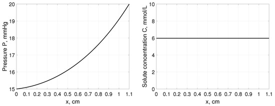
Figure 1.
Interstitial pressure P (left panel) and solute concentration C (right panel) as a function of distance, x, measured from cm, for a tissue stretched from 1 cm to 1.1 cm assuming that , and mmHg [35].
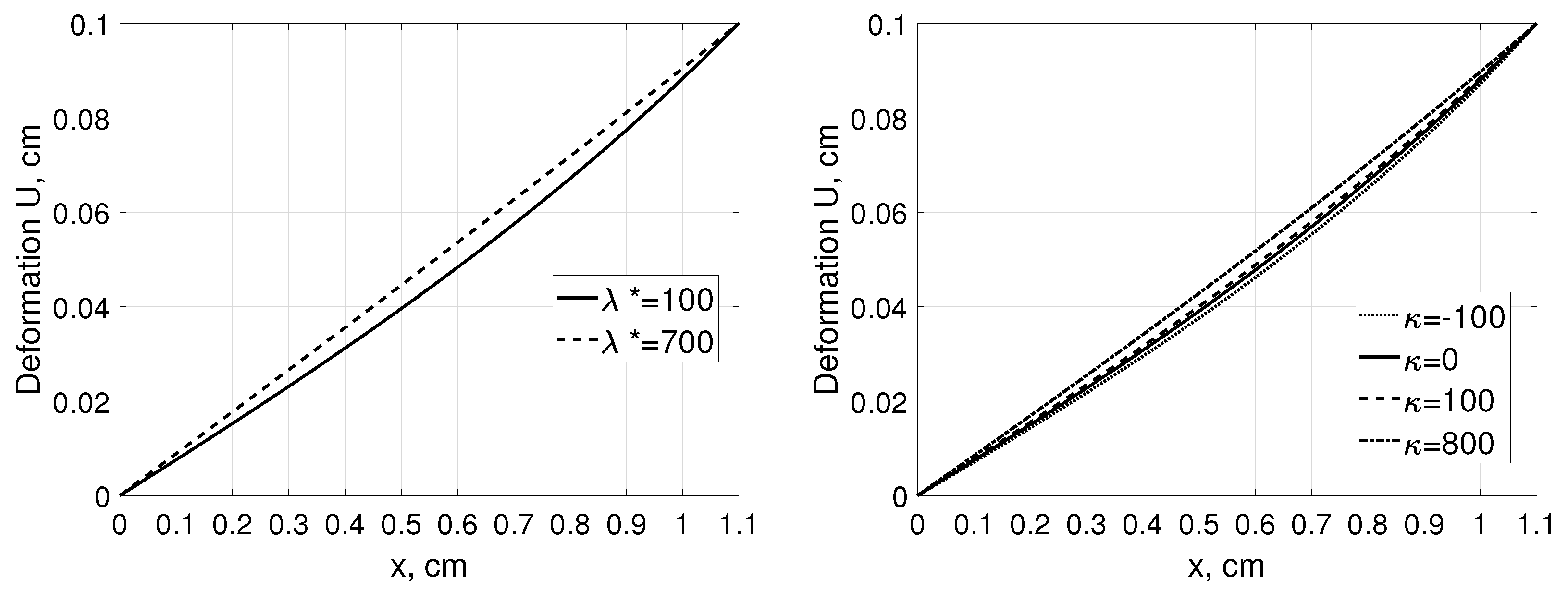
Figure 2 shows corresponding displacement profiles as a function of distance from for a given tissue deformation. On the contrary to the pressure and concentration profiles, local tissue displacement depends on the Terzaghi stress tensor parameters. In the Figure 2 (left pane), difference in the deformation profile between connective (, [6]) and tumor tissue () was presented whereas impact of nonlinear part of stress tensor on the local tissue displacement is presented in Figure 2 (right panel).
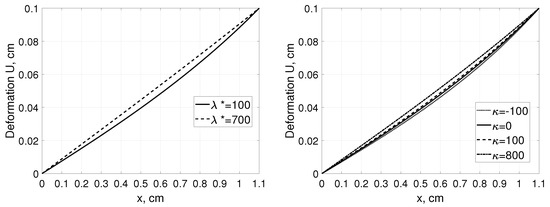
Figure 2.
Deformation U as a function of distance, x, measured from for a tissue stretched from 1 cm to 1.1 cm assuming that that , and mmHg [35]. Left panel: connective () and tumor tissue () assuming , and right panel: for different values assuming .
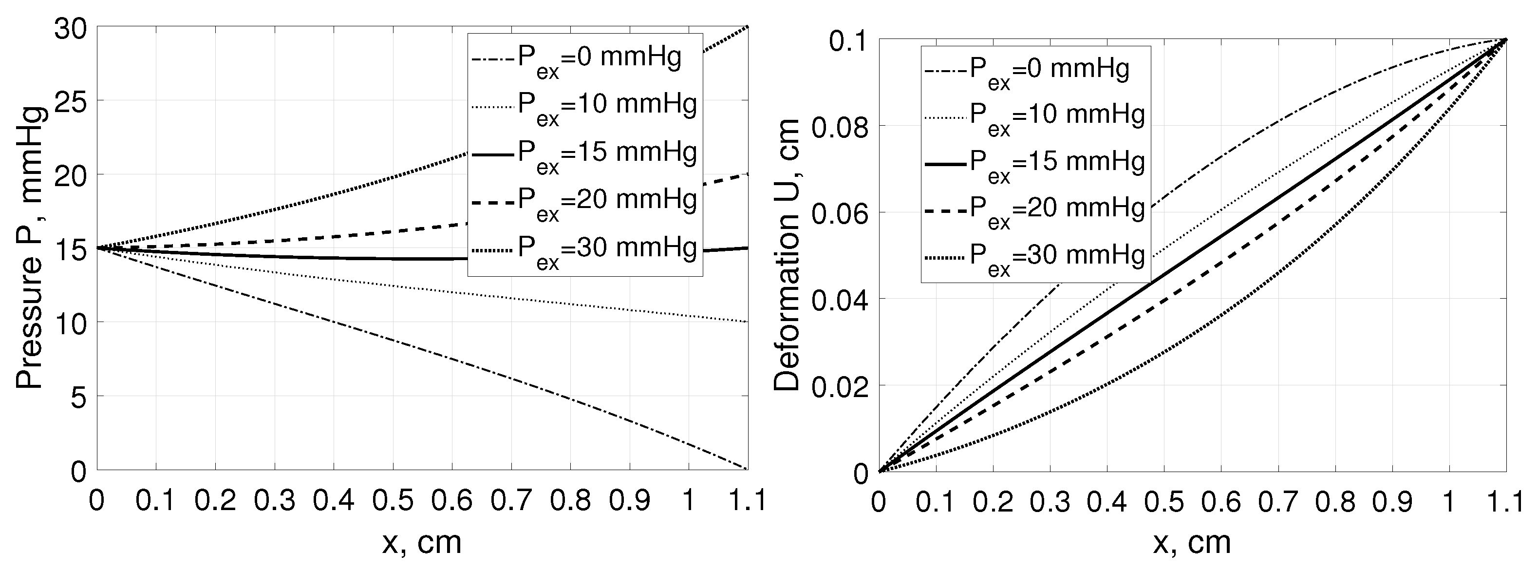
Moreover, even assuming the same value of tissue stretching, i.e., having cm but applying various external hydrostatic pressures mmHg we are getting different interstitial pressure and deformation profiles within the tissue as presented in Figure 3.
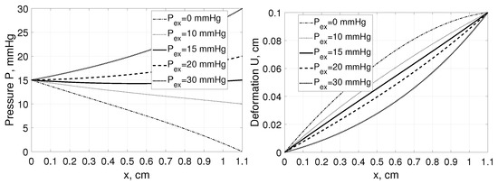
Figure 3.
Interstitial pressure P (left panel) and tissue deformation U (right panel) as a function of distance, x, measured from for a tissue stretched from 1 cm to 1.1 cm assuming , and , mmHg [35].
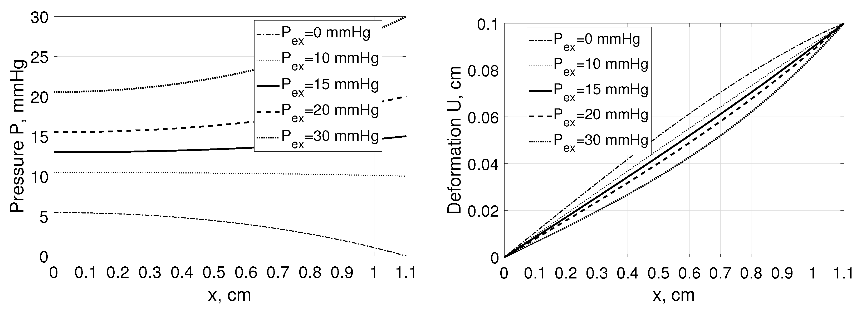
Example 2. Let us consider the basic Equations (15) with boundary conditions
Mathematically it means that we consider the zero Neumann conditions at the boundary , i.e., no-flux conditions.
Let us specify the parameters in the exact solution (20), which guarantee that formulae (20) give the exact solution of BVP (15) and (30). Obviously, the parameters for the concentration should again satisfy the restriction (31). So, making similar calculations one shows that solution (20) satisfies conditions (32) if the constants and have the forms
In the case and the additional restriction takes place, integral in (20) can be expressed in the terms of elementary functions, hence we obtain
Thus, the boundary condition leads to the formula for
Due to the Neumann boundary condition at the left boundary any changes of the would lead not only to the substantial changes in the interstitial pressure profiles (similarly to the Example 1) but also to those in P in the point , whereas the related changes in the deformation profiles would be relatively small, see Figure 4.
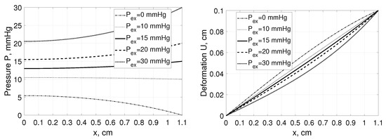
Figure 4.
Interstitial pressure P (left panel) and tissue deformation U (right panel) as a function of distance, x, measured from for a tissue stretched from 1 cm to 1.1 cm assuming , and , mmHg with parameters for solute transport as in Example 1 [35].
Example 3. Let us consider in contrast to Example 1, a small shrinkage of tissue from cm to cm assuming that pressures at the boundaries are the same as in Example 1. Figure 5 shows that in case of more elastic properties of the material (), the impact of the boundary conditions (higher pressure closely to , as in Figure 1, left profile but for cm instead of cm) on the local tissue deformation U is more pronounced. Further increase of tissue shrinkage to cm leads to smaller difference in the tissue displacement between considered materials with different elastic properties, Figure 5, right panel. In both cases, the relevant simulations have also showed that the impact of nonlinear term of stress tensor, , on the local displacement or pressure profile was negligible.
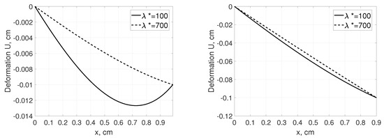
Figure 5.
Deformation U as a function of distance, x, measured from for a tissue from 1 cm to 0.99 cm (smaller shrinkage, left panel) and from 1 cm to 0.90 cm (larger shrinkage, right panel). The parameters are taken as follows , mmHg, , (connective tissue) and (tumor tissue).
5. Discussion
Notably, our previous analysis considered nonperfused material and linear theory of poroelasticity [21]. The model presented here describe transport of fluid and solutes through the perfused tissue providing information on the changes in the hydrostatic pressure and solute concentration profiles in the tissue, and tissue deformation with a nonlinear term in the Terzaghi stress tensor [2,21,23]. The model for perfused tissue, which takes into account the local exchange between tissue and blood and lymphatic systems, is based on the system of nonlinear PDEs. Since the latter is nonintegrable, we applied the method of Lie symmetry analysis in order to identify its properties. It was established that the system possesses nontrivial properties depending on values of densities of the fluxes , and the solute flux (Section 2). Here we used the simplest Lie symmetry that allows us to construct steady-state solutions, which are very important for the model in question. The relevant nonlinear ODE system was treated in details in order to provide closed formulae for steady-state solutions. In particular, the effect of nonlinear term in the Terzaghi stress tensor was studied (Section 3). Notably, some additional restrictions on the parameters were needed, otherwise steady-state solutions cannot be derived explicitly. Interestingly that the restriction was also used in our earlier papers [34,35], where the model has an essentially different structure.
The steady-state solutions obtained allowed us to present two realistic examples. An analysis of the impact of the parameter values and boundary conditions on the distribution of hydrostatic pressure, osmotic agent and displacement in the perfused tissue was provided (Section 4). In particular, the effect of nonlinear term in the Terzaghi stress tensor on the displacement may be evaluated (Figure 2). Thus, the solutions derived provide the insight into the role of some model parameters in the described transport and displacement processes, assuming some simplifications in the description of those physiologically and mathematically complex problems that need in general numerical approach and specification of all model parameters.
In a forthcoming paper we plan to construct time-dependent solutions of the model using the Lie symmetries identified above and to provide more complicated examples of their applications.
Author Contributions
Conceptualization and methodology, R.C. and J.W.; investigation R.C., V.D., J.S.-P. and J.W.; software, V.D. and J.S.-P.; formal analysis, V.D.; data preparation and analysis, J.S.-P.; writing—original draft preparation, R.C., J.S.-P. and J.W.; writing—review and editing, V.D. and J.S.-P. All authors read and agreed to the published version of the manuscript.
Funding
This research was partially supported by NAS of Ukraine and Polish AS within the joint project ‛Mathematical models of hydration-related structural tissue deformations’.
Conflicts of Interest
The authors declare no conflict of interest.
References
- Hall, J.E. Guyton and Hall Textbook of Medical Physiology, 13th ed.; Elsevier: Philadelphia, PA, USA, 2016. [Google Scholar]
- Loret, B.; Simoes, F.M.F. Biomechanical Aspects of Soft Tissue; CRC Press: Boca Raton, FL, USA, 2017. [Google Scholar]
- Stachowska-Pietka, J.; Waniewski, J.; Flessner, M.F.; Lindholm, B. Concomitant bidirectional transport during peritoneal dialysis can be explained by a structured interstitium. Am. J. Physiol. Heart Circ. Physiol. 2016, 310, H1501–H1511. [Google Scholar] [CrossRef] [Green Version]
- Netti, P.A.; Baxter, L.T.; Boucher, Y.; Skalak, R.; Jain, R.K. Time dependent behavior of interstitial fluid in solid tumors: Implications for drug delivery. Cancer. Res. 1995, 55, 5451–5458. [Google Scholar] [PubMed]
- Leiderman, R.; Barbone, P.E.; Oberai, A.A.; Bamber, J.C. Coupling between elastic strain and interstitial fluid flow: Ramifications for poroelastic imaging. Phys. Med. Biol. 2006, 51, 6291–6313. [Google Scholar] [CrossRef]
- Swartz, M.A.; Kaipainen, A.; Netti, P.A.; Brekken, C.; Boucher, Y.; Grodzinsky, A.J.; Jain, R.K. Mechanics of interstitial-lymphatic fluid transport: Theoretical foundation and experimental validation. J. Biomech. 1999, 32, 1297–1307. [Google Scholar] [CrossRef]
- Waniewski, J.; Stachowska-Pietka, J.; Flessner, M.F. Distributed modeling of osmotically driven fluid transport in peritoneal dialysis: Theoretical and computational investigations. Am. J. Physiol. Heart Circ. Physiol. 2009, 296, H1960–H1968. [Google Scholar] [CrossRef] [Green Version]
- Stachowska-Pietka, J.; Poleszczuk, J.; Flessner, M.F.; Lindholm, B.; Waniewski, J. Alterations of peritoneal transport characteristics in dialysis patients with ultrafiltration failure: Tissue and capillary components. Nephrol. Dial. Transplant. 2019, 34, 864–870. [Google Scholar] [CrossRef]
- Flessner, M.F. Transport of protein in the abdominal wall during intraperitoneal therapy. I. Theoretical approach. Am. J. Physiol. Gastrointest. Liver. Physiol. 2001, 281, G424–G437. [Google Scholar] [CrossRef]
- Wiig, H.; Swartz, M.A. Interstitial fluid and lymph formation and transport: Physiological regulation and roles in inflammation and cancer. Physiol. Rev. 2012, 92, 1005–1060. [Google Scholar] [CrossRef] [PubMed]
- Malakpoor, K.; Kaasschieter, E.F.; Huyghe, J.M. Mathematical modelling and numerical solution of swelling of cartilaginous tissues. Part I: Modelling of incompressible charged porous media. Esaim-Math. Model. Numer. Anal.-Model. Math. Anal. Numer. 2007, 41, 661–678. [Google Scholar] [CrossRef] [Green Version]
- Cortes, D.H.; Jacobs, N.T.; DeLucca, J.F.; Elliott, D.M. Elastic, permeability and swelling properties of human intervertebral disc tissues: A benchmark for tissue engineering. J. Biomech. 2014, 47, 2088–2094. [Google Scholar] [CrossRef] [Green Version]
- Stokes, I.A.F.; Laible, J.P.; Gardner-Morse, M.G.; Costi, J.J.; Iatridis, J.C. Refinement of Elastic, Poroelastic, and Osmotic Tissue Properties of Intervertebral Disks to Analyze Behavior in Compression. Ann. Biomed. Eng. 2011, 39, 122–131. [Google Scholar] [CrossRef] [Green Version]
- Lai, W.M.; Hou, J.S.; Mow, V.C. A triphasic theory for the swelling and deformation behaviors of articular cartilage. J. Biomech. Eng. 1991, 113, 245–258. [Google Scholar] [CrossRef]
- Schuff, M.M.; Gore, J.P.; Nauman, E.A. A mixture theory model of fluid and solute transport in the microvasculature of normal and malignant tissues. I. Theory. J. Math. Biol. 2013, 66, 1179–1207. [Google Scholar] [CrossRef] [PubMed]
- Netti, P.A.; Baxter, L.T.; Boucher, Y.; Skalak, R.; Jain, R.K. Macro- and microscopic fluid transport in living tissues: Application to solid tumors. AIChE J. 1997, 43, 818–834. [Google Scholar] [CrossRef]
- Kellen, M.R.; Bassingthwaighte, J.B. An integrative model of coupled water and solute exchange in the heart. Am. J. Physiol. Heart Circ. Physiol. 2003, 285, H1303–H1316. [Google Scholar] [CrossRef] [PubMed] [Green Version]
- Flessner, M.F.; Dedrick, R.L.; Schultz, J.S. A distributed model of peritoneal-plasma transport: Theoretical considerations. Am. J. Physiol. 1984, 246, R597–R607. [Google Scholar] [CrossRef]
- Stachowska-Pietka, J.; Waniewski, J. Distributed modeling of glucose induced osmotic fluid flow during single exchange with hypertonic glucose solution. Bioc. Biomed. Eng. 2011, 31, 39–50. [Google Scholar]
- Stachowska-Pietka, J.; Naumnik, B.; Suchowierska, E.; Gomez, R.; Waniewski, J.; Lindholm, B. Water removal during automated peritoneal dialysis assessed by remote patient monitoring and modelling of peritoneal tissue hydration. Sci. Rep. 2021, 11, 15589. [Google Scholar] [CrossRef]
- Cherniha, R.; Stachowska-Pietka, J.; Waniewski, J. A Mathematical Model for Transport in Poroelastic Materials with Variable Volume: Derivation, Lie Symmetry Analysis, and Examples. Symmetry 2020, 12, 396. [Google Scholar] [CrossRef] [Green Version]
- Schmid-Schonbein, G.W. Microlymphatics and lymph flow. Physiol. Rev. 1990, 70, 987–1028. [Google Scholar] [CrossRef] [PubMed]
- Taber, L.A. Nonlinear Theory of Elasticity. Applications in Biomechanics; World Scientific: Hackensack, NJ, USA, 2004. [Google Scholar]
- Detournay, E.; Cheng, A.H.-D. Fundamentals of poroelasticity. Chap. 5 in Comprehensive Rock Engineering: Principles, Practice and Projects. In Analysis and Design Methods; Pergamon Press: Oxford, UK, 1993; Volume II. [Google Scholar]
- Bluman, G.W.; Cheviakov, A.F.; Anco, S.C. Applications of Symmetry Methods to Partial Differential Equations; Springer: New York, NY, USA, 2010. [Google Scholar]
- Arrigo, D.J. Symmetry Analysis of Differential Equations; John Wiley & Sons: Hoboken, NJ, USA, 2015. [Google Scholar]
- Cherniha, R.; Serov, M.; Pliukhin, O. Nonlinear Reaction-Diffusion-Convection Equations: Lie and Conditional Symmetry, Exact Solutions and Their Applications; Chapman and Hall/CRC: New York, NY, USA, 2018. [Google Scholar]
- Patera, J.; Winternitz, P. Subalgebras of real three- and four-dimensional Lie algebras. J. Math. Phys. 1977, 18, 1449–1455. [Google Scholar] [CrossRef]
- Polyanin, A.D.; Zaitsev, V.F. Handbook of Ordinary Differential Equations: Exact Solutions, Methods, and Problems; CRC Press: Boca Raton, FL, USA, 2018. [Google Scholar]
- Ovsiannikov, L.V. Group Analysis of Differential Equations; Academic Press: New York, NY, USA, 1982. [Google Scholar]
- Cherniha, R.; Serov, M.; Prystavka, Y. A complete Lie symmetry classification of a class of (1+2)-dimensional reaction-diffusion-convection equations. Commun. Nonlinear Sci. Numer. Simulat. 2021, 92, 105466. [Google Scholar] [CrossRef]
- Torrisi, M.; Traciná, R. Lie Symmetries and Solutions of Reaction Diffusion Systems Arising in Biomathematics. Symmetry 2021, 13, 1530. [Google Scholar] [CrossRef]
- Stachowska-Pietka, J.; Waniewski, J.; Flessner, M.F.; Lindholm, B. A distributed model of bidirectional protein transport during peritoneal fluid absorption. Adv. Perit. Dial. 2007, 23, 23–27. [Google Scholar]
- Cherniha, R.; Gozak, K.; Waniewski, J. Exact and numerical solutions of a spatially-distributed mathematical model for fluid and solute transport in peritoneal dialysis. Symmetry 2016, 8, 50. [Google Scholar] [CrossRef] [Green Version]
- Cherniha, R.; Stachowska-Pietka, J.; Waniewski, J. A mathematical model for fluid-glucose-albumin transport in peritoneal dialysis. Int. J. Appl. Math. Comp. Sci. 2014, 24, 837–851. [Google Scholar] [CrossRef] [Green Version]


Publisher’s Note: MDPI stays neutral with regard to jurisdictional claims in published maps and institutional affiliations. |
© 2022 by the authors. Licensee MDPI, Basel, Switzerland. This article is an open access article distributed under the terms and conditions of the Creative Commons Attribution (CC BY) license (https://creativecommons.org/licenses/by/4.0/).