Article

Rolling Bearing Fault Diagnosis Based on Deep Learning and Autoencoder Information Fusion

1
School of Instrumentation Science and Engineering, Harbin Institute of Technology, Harbin 150001, China
2
Songsim Global Campus, Undergraduate College, The Catholic University of Korea, Bucheon-si 14662, Gyeonggi-do, Korea
*
Author to whom correspondence should be addressed.
Symmetry 2022, 14(1), 13; https://doi.org/10.3390/sym14010013
Submission received: 13 November 2021 / Revised: 15 December 2021 / Accepted: 18 December 2021 / Published: 23 December 2021

Abstract

:
The multisource information fusion technique is currently one of the common methods for rolling bearing fault diagnosis. However, the current research rarely fuses information from the data of different sensors. At the same time, the dispersion itself in the VAE method has asymmetric characteristics, which can enhance the robustness of the system. Therefore, in this paper, the information fusion method of the variational autoencoder (VAE) and random forest (RF) methods are targeted for subsequent lifetime evolution analysis. This fusion method achieves, for the first time, the simultaneous monitoring of acceleration signals, weak magnetic signals and temperature signals of rolling bearings, thus improving the fault diagnosis capability and laying the foundation for subsequent life evolution analysis and the study of the fault–slip correlation. Drawing on the experimental procedure of the CWRU’s rolling bearing dataset, the proposed VAERF technique was evaluated by conducting inner ring fault diagnosis experiments on the experimental platform of the self-research project. The proposed method exhibits the best performance compared to other point-to-point algorithms, achieving a classification rate of 98.19%. The comparison results further demonstrate that the deep learning fusion of weak magnetic and vibration signals can improve the fault diagnosis of rolling bearings.

1. Introduction

Rolling bearings are widely used in civil and military industries because of their high interchangeability, low frictional resistance, low power consumption and high transmission efficiency [1,2]. At the same time, damage to rolling bearings may lead to the complete failure of mechanical equipment and even cause economic loss including human casualties [3,4].
The condition of a rolling bearing can be determined by measuring vibration [5], acoustic [6], thermal [7] and oil-based [8] signals. However, these measurements do not reflect the speed of the cage of the rolling bearing during operation. Thus, it is not possible to investigate the results related to the life evolution analysis regarding slippage and failure during the full life cycle. At the same time, the common methods for monitoring the cage speed are not perfect. For example, the electromagnetic induction detection [9] method requires a high electromagnetic field strength; therefore, the bearing must be magnetized before detection can be performed. This may lead to a buildup of metal debris dislodged by friction during bearing operation, which accelerates bearing failure and reduces bearing life. In the pulsed laser [10] and photoelectric sensor [11] methods, the bearings are lubricated with the provided oil, or the cage is encased in grease and the bearings are lubricated. The high-speed rotation and the increase in bearing temperature may lead to the accumulation of oil mist laced with impurities in the cavity. However, due to the detection principles involved in these two methods, oil mist and obstructions are indistinguishable. The strain gauge method [12] destroys the structure of the bearing and does not objectively reflect the true usage of the bearing. The ultrasonic inspection method [13] requires the outer ring of the bearing to be close to the sensor; it also requires the use of a coupling agent. Therefore, these necessary conditions make it difficult to implement this technique in engineering applications. Currently, cage speed is rarely included as one of the measurement results in the field of multisensor information fusion fault diagnosis. Cage rotational speed has been considered only in the study of dynamic simulation models that unify rotational speed and faults with slippage, and the relationship between them is formulated through theoretical calculations [14]. In summary, in order to fill the gaps in the current study and to pave the way for the subsequent life evolution analysis, the aim of this paper is to propose an information fusion method that unifies the cage speed measurement signal with the fault and temperature signals for fault diagnosis to improve the diagnostic accuracy. In terms of cage speed measurement, a weak magnetic detection method [15] is a recently proposed non-contact technique for measuring rolling bearing cage speed, which is used in this work. The method is based on the fact that the rolling body and inner ring, as magnetic conductors, are weakly magnetic in the presence of the geomagnetic field and cause weak periodic changes in the surrounding geomagnetic field during the rotation of the bearing. Therefore, the purpose of measuring the rotational frequency of the rolling element, cage and inner ring of the bearing can be achieved with a weak magnetic sensor in a non-contact situation [15].
The current research on bearing fault diagnosis based on multisensor information fusion is mainly focused on the research of the information fusion algorithm under the use of multiple acceleration sensors to collect vibration signals. For example, Gao et al. used the rolling bearing fault diagnosis method based on the entropy fusion feature of complementary ensemble empirical mode decomposition [16]. Hoang et al. observed that the convolutional neural network processed multiple signal sources simultaneously and was constrained by sensor functions [17]. Jiao et al. proposed a new bearing fault diagnosis method based on the least squares support vector machine for feature-level fusion and the Dempster–Shafer (DS) evidence theory for decision-level fusion [18]. Song et al. proposed a multisensor data fusion classification method [19] based on linear discriminant analysis for feature classification. It evaluated corresponding fluctuations detrended by locally fitting vibration signals using an improved detrended wave analysis and selected wave function polynomial fitting coefficients as fault features. Tang et al. proposed an improved DS evidence theory fusion method based on Cohen’s kappa coefficient to solve the bearing fault diagnosis problem [20]. Soualhi et al. proposed an adaptive neuro-fuzzy inference system to study bearing multisource information fusion [21]. Liu et al. proposed an integrated convolutional neural network model to study multisensor information fusion [22]. Kamat et al. proposed a deep learning method for remaining life assessment of bearings [23]. Sayyad et al. presented a data-driven analysis of remaining life estimation based on a comprehensive description of monitoring methods, algorithms, and future challenges and opportunities [24].
Up to now, Safizadeh et al. used accelerometers and load cells to collect signals simultaneously for bearing fault diagnosis by means of information fusion [25]. In 2021, Safizadeh et al. implemented information fusion for rolling bearings using an accelerometer and a microphone. In addition, they performed feature extraction by principal component analysis (PCA) and decision fusion using the K-nearest neighbor method in the classification module [26]. Li et al. investigated rolling bearing information fusion using oil analysis data, microscopic debris analysis data, and vibration data. However, microscopic debris analysis data and oil analysis data in this method belong to image processing as well as physical and chemical analysis [27]. Gunerkar et al. performed bearing fault diagnosis by using the information fusion of acceleration and acoustic emission sensors [28]. Wang et al. proposed a single-dimensional convolutional neural network (CNN) method to fuse acoustic vibration data for bearing fault diagnosis [29]. Most of the above methods are conventional methods and all of them are different methods to diagnose the same fault, so there has not been a precedent for the fusion of cage speed signals with fault signals. There are also some papers that apply information fusion methods to different fields [30,31].
A comprehensive analysis of previous studies shows that no information fusion algorithm has been developed to reflect the relationship between bearing failure and slippage, or to fuse the sensor signals from both in the form of a test. In addition, current research on information fusion requires the manual addition of data tags; this is both time consuming and labor intensive. As a result, only a small amount of information in the dataset is labeled, whereas a considerable amount of unlabeled data cannot be trained to improve model performance. Data-feature extraction yields time-series information. In previous studies, fault prediction could only be implemented after feature-value extraction (e.g., using windowed fast Fourier transform or wavelet transform to extract frequency domain information). Feature extraction itself causes information loss. Moreover, since data-feature extraction and prediction-model training are two separate processes, information loss is inevitably exacerbated, thus degrading the model performance. Typically, previous studies have only used the same type of data. In contrast, in this paper, data from cage speed and acceleration sensors are collected for the first time, and a deep learning algorithm for fusing the information is purposefully proposed.
The main innovative work of this paper is: (1) the first application of the weak magnetic detection method to the whole life cycle monitoring of rolling bearings. (2) For the subsequent life evolution analysis study, an information fusion algorithm is proposed for the first time for the weak magnetic detection method with the fault signal and temperature signal. (3) In this paper, inspired by the literature [32], the operation of the VAE model herein is improved for the multi-sensor information fusion problem used in this paper, and its proposed fault diagnosis method is extended to multisource information fusion for fault diagnosis and life evolution analysis. With the asymmetry of the VAE algorithm, the robustness of the information fusion process can be better improved.
Section 2 of this paper presents related works. Section 3 presents the proposed multisource information fusion algorithm in this paper. Section 4 describes the engineering experimental study, and Section 5 summarizes the conclusions of the study.

2. Background Theory

2.1. Variational Autoencoders

An autoencoder (AE) model is a self-supervised learning model that can generate data samples similar to training data [33]. This model generally consists of an encoder and a decoder. The encoder can analyze hidden features of input data and compress them into potential hidden space, whereas the decoder can reconstruct the initial input data from the potential space based on low-dimensional features learned during the model training. After repeated training, the autoencoder attempts to copy the input data to the output data. However, if the autoencoder is designed to have equal input and output, its role is completely eliminated. In practical application, the input data must be approximately equal to the output data. To achieve this, additional conditions that can constrain the data in the autoencoder such that they are only approximately optimized are required. By introducing these constraints, the autoencoder can learn effective data feature representation.
A variational autoencoder (VAE) is also a type of automatic encoder. In 2013, Kingma et al. [34] proposed a typical generation model VAE capable of effectively fitting and learning complex probability distributions. Similar to the structure of autoencoders, the VAE also consists of an encoder and a decoder; it is a combination of variational inference and a neural network. A significant difference between VAE and AE is the existence of variational derivation [35]. Here, an approximate distribution, p ( z k ) , for replacing a distribution, q ϕ ( z k | x k ) , which is generated by the encoder function, is found. The similarity between the two distributions is measured by the Kullback–Leibler (KL) divergence [36]. During training, the encoder maps the input data to the hidden variable space, where the variables generally follow the standard normal probability distribution. The decoder reconstructs the information by sampling data in the middle hidden variable space. As a deep learning model, the VAE combines the technical characteristics of statistical learning and deep learning well. Thus, it has exceptional nonlinear fitting ability and is an excellent generation model.
In practice, the VAE requires balance between model accuracy and hidden vector compliance with standard normal distribution. Model accuracy, as determined by the network, refers to the similarity between decoder-generated data and original input data. By considering the difference between the two as the total loss, the network can determine how it can be reduced. This loss is the mean square error of the generated data and original data. In addition, calculating the similarity in the distribution of the two hidden variables using the KL divergence is necessary. The VAE algorithm training process is given by Algorithm 1.
Algorithm 1 VAE algorithm
Input: data D = { x 1 , x 2 , , x n }
Output: Probability Encoder E, Probability Decoder D
1. ϕ and θ are initialization parameters;
2. Repeat:
3. For i = 1 to n do
4. Take L samples from ε N ( 0 , 1 )
5. z ˜ = h ϕ ( ε , x )
6. End for
7. E = i = 1 N D K L ( q ϕ ( z | x ( i ) ) p θ ( z ) ) + 1 L l = 1 L ( log p θ ( x ( i ) | z ( i , l ) ) )
8. ϕ and θ are updated parameters by random gradient descent
9. Until parameters ϕ and θ converge
The specific calculation of the VAE generation model is as follows:
Assume that input data are represented by x , and the hidden variable is z ; simplify the model using Max-Log-MAP. The following is obtained according to Bayes’ formula:
p ( z | x ) = p ( x | z ) p ( z ) z p ( x | z ) p ( z ) d z
For a complex model with a considerable data scale, solving the above formula is difficult. To overcome this problem, the variational method can be adopted to replace p ( z | x ) with a variational function, q ( z | x ) . The two probability distributions must be as similar as possible. To calculate the similarity between the two, the K L divergence is applied. The following is obtained according to the K L divergence formula:
K L ( q ( z | x ) p ( z | x ) ) = q ( z | x ) [ log q ( z | x ) log p ( z | x ) ] d z
Transforming the foregoing according to Bayes’ formula yields:
= q ( z | x ) [ log q ( z | x ) log p ( x | z ) log p ( z ) + log p ( x ) ] d z
Because the objective of the integral is z , terms unrelated to z are removed from the integrand and simplified, as follows:
log p ( x ) K L ( q ( z | x ) p ( z | x ) ) = q ( z | x ) log ( p | x ) d z K L ( q ( z | x ) p ( z ) )
The objective of model training is to reduce K L ( q ( z | x ) p ( z | x ) ) to the smallest quantity possible. This means that the right-hand side of the formula must be increased to the greatest extent feasible. The first term on this side is actually the logarithmic likelihood expectation based on probability q ( z | x ) ; the second term is a negative KL divergence. A satisfactory value of q ( z | x ) that is as close as possible to p ( z | x ) must be found to achieve the final optimization objective. The optimization objectives are the log likelihood expectation maximization of the first term and the KL divergence minimization of the second term on the right-hand side.
To solve the above formula, the reparameterization technique is applied. For example, a Gaussian random variable, a , with a mean and variance of 1 can be represented by a random variable with a mean of 0 and a variance of 1 plus a constant, 1. Then, the random variable is divided into specific and random parts. Thus, q ( z | x ) can be divided into two parts. One part is the observable variable, g ϕ ( x ) , representing the deterministic part of the conditional probability and which is similar to the expected value of a random variable; the other part is the random variable, ε . If z ( i ) = g ϕ ( x + ε ( i ) ) , then q ( z ( i ) | x ) = p ( ε ( i ) ) , then the above formula transforms to the following:
log p ( x ) K L ( q ( z | x ) p ( z | x ) ) = p ( ε ) log p ( x | g ϕ ( x , ε ) ) d z K L ( q ( z | x , ε ) p ( z ) )
Having determined the distribution of z by ε , modeling the variational function is completed by assuming that ε follows a certain distribution. The conditional distribution of z is learned according to the training data. This is because the distribution of z may considerably vary after calculating g ϕ ( x ) , which can be expressed by the deep learning model. Thus, in the VAE, ε follows a multidimensional Gaussian distribution, the dimensions of which are independent of each other. Moreover, the prior and posterior distributions of z are assumed to have the same distribution and dimensional independence.
The second optimization objective is the minimization of the second term, K L ( q ( z | x , ε ) p ( z ) ) , on the right-hand side of the formula. Because the prior distribution of z is assumed to be the multidimensional Gaussian distribution with the dimensions independent of each other, the variational autoencoder provides a stronger assumption; that is, it follows the standard Gaussian distribution. Consequently, the KL divergence formula above is easier to calculate. As mentioned above, for g ϕ ( x , ε ) in a deep network, the input is accumulated data, x , and the output is z , which is generated by x . Their mean and variance are obtained by a data summary calculation. Function g ϕ ( x ) is called an encoder model because it converts observable data into hidden variables.
The first optimization objective is to maximize the likelihood expectation of the first term on the left-hand side of the formula. Because the encoder model has calculated the hidden variable, z , corresponding to the observable variable, x , another deep model can be formulated. It is based on the likelihood in which the input is the hidden variable, z , and the output is the observed variable, x . If the output data are similar to the previous input data, the likelihood can be considered maximized. Consequently, the decoder, which is a generative model, is formulated.
The VAE can be expressed by the following formulae:
log p θ ( x ) E q ϕ ( z | x ) [ log ( x | z ) ] K L ( q ϕ ( z | x ) p ( z ) )
x ^ = f e n c ( x )
q ϕ ( z | x ) = N ( μ ( x ^ ) , d i a g ( σ 2 ( x ^ ) ) )
z q ϕ ( z | x )
p θ ( x | z ) = D ( x | f d e c ( z ) )
The VAE consists of an encoder and a decoder, corresponding to q ϕ ( z | x ) and p θ ( x | z ) , respectively. Moreover, f e n c ( x ) and f d e c ( z ) can be implemented by various neural network models, such as multilayer perception or long short-term memory. The VAE network model is shown in Figure 1, which illustrates several key pieces of information, such as the posterior mean and log variance of Gaussian distribution in hidden space.

2.2. Random Forest

Random forest is a supervised learning algorithm with a bagging algorithm that combines many decision trees for classification using a voting mechanism [37]. It has a fast training speed, strong generalization ability, and satisfactory classification performance.
The decision tree, also known as the classification and regression tree (CART), can be used to describe the various classes or values that are outputted after entering a set of features. It is a tree structure in which each inner node represents an attribute test, each branch represents a test output, and each leaf node represents the final test result [38].
Assume that X is an input vector containing m features, Y is an output value, and S n is a training set containing n observed values ( X i , Y i ) . Here, S n is given by:
S n = { ( X 1 , Y 1 ) , , ( X n , Y n ) } , X R m , Y R
During training, the algorithm breaks up the input at each node. First, the CART algorithm recursively divides the input space, X , into two distinct branches:
{ X j < d } { X j > d } , j { 1 , 2 , , m } , d R
For better partitioning, the cost function must be minimized by ( j , d ) , which is usually a variance of child nodes. The variance of node p is defined as:
V a r ( p ) = i : X i p ( Y i Y ¯ p ) 2
where Y ¯ p is the mean of Y i in node p , and the child nodes are divided in the same way. The tree stops growing when the maximum number of levels is reached or when the number of observations in the nodes is less than the predetermined number. At the end of training, a prediction function, h ^ ( X , S n ) , based on S n is established.
For any new input vector, X , the prediction function can yield a prediction, Y ^ (related to output Y ), given by:
Y ^ = h ^ ( X , S n )
Random forest is an integration method that combines multiple decision trees. It extracts multiple samples from original samples through the bootstrap sampling method and builds a decision tree model according to each bootstrap sample. Then, the algorithm integrates the prediction of multiple decision trees and obtains the final result by voting. Random forest regression can be regarded as a strong predictive factor for integrating many weak predictive factors.
A bootstrap sample is obtained by randomly selecting n observation data replaced from the original dataset, S n . The random forest algorithm selects several bootstrap sub-datasets ( S n 1 , , S n q ) to which CART is applied. Some trees are formed, and prediction functions, such as Formula (14), are obtained.
The random forest algorithm also selects m t r y features from all m features for segmenting the nodes of all trees. Here, m t r y is a predefined number, which is usually the square root or one third of the number of features, m . The random forest algorithm finds the best segmentation point for each tree among the features selected by m t r y . The rest of the algorithm is similar to CART. Finally, the result is obtained by averaging the output of all trees. Thus, the predicted output, Y ^ , obtained from a new input vector, X , is as follows:
Y ^ = 1 q i = 1 q h ^ ( X , S n l )
The random forest process is implemented as follows:
(1)
The original training dataset is S n . Extract dataset q with n observation values using the bootstrap method to build a decision tree.
(2)
There are m variables. Randomly select m t r y variables from each node of each tree. Then, select the variable with the best classification ability among the m t r y variables to derive the best segmentation point.
(3)
Each tree grows to the fullest extent without any modification.
(4)
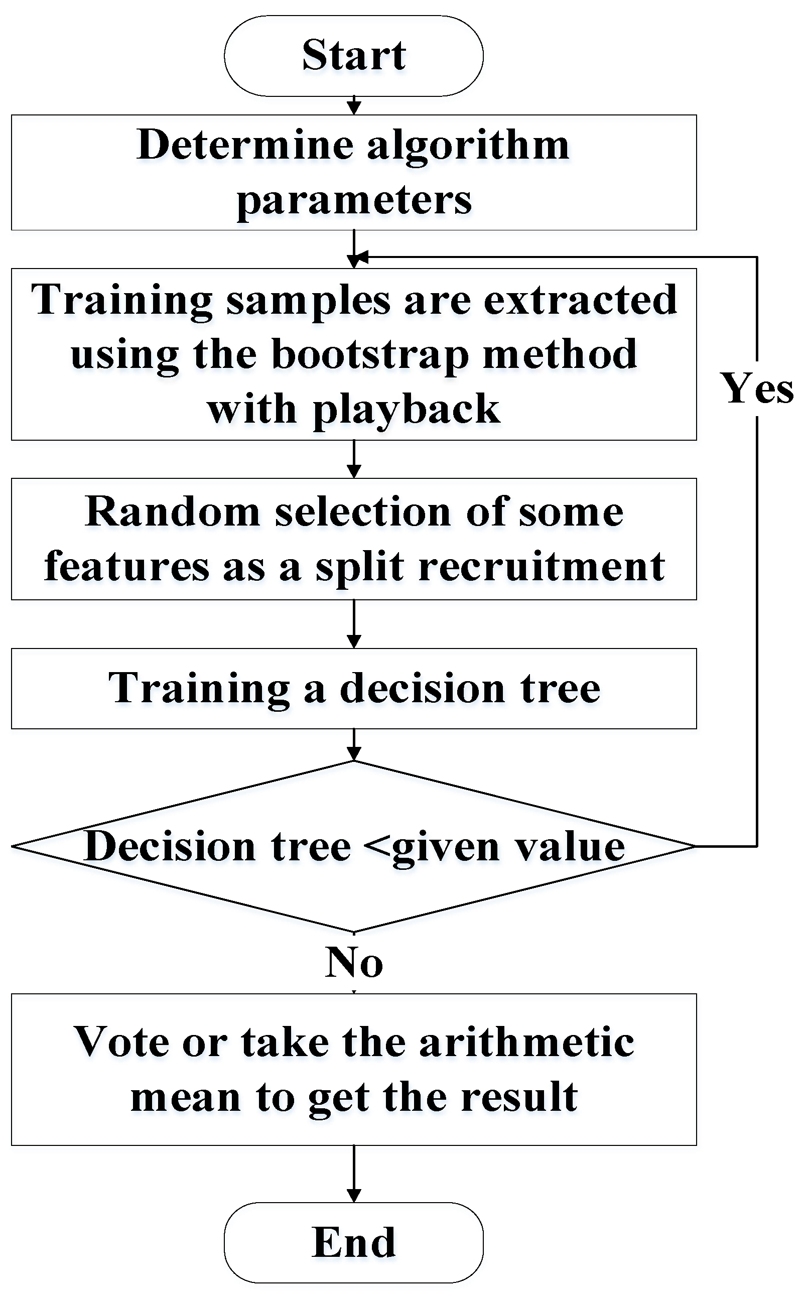
The result tree constructs a random forest to predict new data; the result is determined by the voting of trees in the random forest. Figure 2 shows the random forest algorithm flowchart.
The random forest algorithm has many advantages. For example, because of random sampling, it has strong generalization ability and is easy to implement. Moreover, due to the random selection of features and observations, the algorithm remains effective even when the feature dimension is high.

2.3. Dynamic Simulation Model

The dynamic simulation theory used in the current work refers to the concept formulated in the study of Tu, in 2021, ref. [14] in which the aircraft bearing temperature field is simulated.
Currently, many bearing heat generation models are available, each with its own scope of application. In the Palmgren bearing heat generation model, the bearing friction torque, M, includes the viscous friction torque, M 0 , generated by the lubrication and the friction torque, M 1 , generated by the load. Thus,
M = M 0 + M 1
where M 0 is the friction torque (unit: N·mm) related to the bearing type, bearing speed, and lubricating oil property.
When v n 2000 , M 0 = 10 7 f 0 ( v n ) 2 / 3 d m 3 ; when v n < 2000 , M 0 = 160 × 10 7 f 0 d m 3 , where d m is the bearing pitch circle diameter (unit: mm); f 0 is the coefficient related to the bearing type and lubrication mode; n is the bearing speed (unit: r/min); v is the movement viscosity (unit: mm2·s) of the bearing lubricating oil under working conditions; M 1 is the friction torque (unit: N·mm) caused by the load on the bearing and calculated according to the following formula:
M 1 = f 1 p 1 d m
where f 1 is the coefficient related to bearing type and bearing load, and p 1 is the load (unit: N) for calculating the bearing friction torque. After determining the bearing friction torque, the calorific value generated by frictional heating is calculated according to (17):
Q = 1.05 × 10 4 n M ( W )
where n is the bearing speed (unit: r/min), and M is the bearing friction torque (unit: N·mm).
In the total bearing friction torque, the friction torque caused by the spin sliding of rolling elements accounts for the major part of the torque. Different bearing contact angles cause the rolling element to experience different magnitudes of spin friction torque. Moreover, the two parameters are positively correlated. Under bearing working conditions, the calorific value generated by the spin friction torque is extremely large. Hence, the calorific value generated by spin friction in the thermal analysis of bearings cannot be ignored.
The spin friction torque is calculated using
M s = 3 μ Q a 8
where M s is the spin friction torque (unit: N·mm); Q is the normal load (unit: N) between the channel and balls; a is the long axis length (unit: mm) of the contact ellipse; and is the second class of incomplete elliptic integrals.
In calculating the calorific value of bearings, the accuracy and complexity of calculations are foremost. Compared with other methods for calculating the bearing calorific value, the Palmgren method is more accurate. This calculation method is more suitable when the bearing rotates at medium speed and sustains a medium load.
In the Harris [39] bearing heat generation model, Harris believes that many factors affect the friction heat generation of bearings. These include the spin action of the rolling element, the relative movement between the cage and ball, the relative sliding caused by material deformation, the differential sliding between the ball and channel, the viscous friction caused by the lubricating oil, and the friction caused by the load on the bearing under working conditions. The empirical formula can be used to calculate the bearing calorific value when the Harris model is used, as follows:
M = f 1 F b d m + 1.42 × 10 5 ( v 0 n ) 2 / 3 d m 3
where M is the total friction moment (unit: N·mm); f1 is a coefficient determined by the bearing structure and load of the bearing; F b is the equivalent load (unit: N); V 0 is the lubricating oil viscosity (unit: mm2/s); n is the bearing speed (unit: r/min); and d is the middle diameter (unit: mm) of the bearing.
The Harris model [39] is only applicable to high-speed bearings and has certain limitations in calculating the calorific value. In addition, after years of research, the SKF company has derived the theoretical calculation method for the total friction torque, M, of bearings, as follows:
M = ϕ i s h ϕ r s M r r + M s l + M s e a l + M d r a g
where M r r is the rolling friction torque (unit: N·mm); ϕ i s h is the cut-in heat reduction coefficient; M s l is the sliding friction torque (unit: N·mm); ϕ r s is the reduction coefficient of the lean oil backfill; M s e a l is the friction torque (unit: N·mm) of the seal; and M d r a g is the friction torque (unit: N·mm) caused by the lubricating oil (e.g., splash and eddy current).
In addition to the above models for calculating the calorific value of bearings, the approximate calculation formula of the total friction torque of bearings can also be derived according to different bearing types, bearing structures, and operating conditions:
M = 1 2 μ d p
where μ is the friction coefficient of the rolling bearing; d is the bearing inner diameter (unit: mm); and p is the load (unit: N) on the bearing.
For centripetal bearings, P is the radial load, F r , whereas, for thrust bearings, P is the axial load, F a . Centripetal bearings are subject to the joint action of axial and radial forces, as follows:
When F a / F r 1.5 tan α , P = F r ;
When F a / F r > 1.5 tan α , P = 0.4 ( F r + F a cot α )
The foregoing models are not universal for calculating the calorific value of bearings; for different cases, different models must be used. For rolling bearings with medium speed, medium load, and satisfactory lubrication, the Palmgren model is more consistent with the actual condition of bearings to calculate the calorific value. For rolling bearings with relatively high speeds, the Harris model is more suitable for calculating the calorific value, and the calculated results are more consistent with experimental conditions. However, the final calorific values calculated by the Harris and Palmgren models do not significantly differ. For rolling bearings with low speed but considerable load, the most accurate bearing calorific value is calculated by the SKF model. In the spindle experimental platform, the bearings used are angular contact ball bearings. Based on the actual working conditions of bearings and after comparing the advantages and disadvantages of different models, the Palmgren model is selected for calculating the caloric value of bearings.
The heat in bearings is mainly transferred in three ways: thermal convection between bearings and surrounding media; heat conduction between bearing, shaft, and bearing seat; thermal radiation between bearings and bearing parts. Among the three, thermal radiation among bearing components is relatively small and virtually does not affect the calculation of bearing calorific value; hence, it can be ignored. The heat transfer between bearing and lubricating oil is the main means of heat transfer. Therefore, in the study of bearing heat transfer, the convective heat transfer coefficient of bearings must first be determined. Convective heat transfer mainly has two forms: natural convection and forced convection. Harris indicates that the heat transfer coefficient can be calculated according to the following formula:
H v = α S ( T 1 T 2 )
where H v is the calorific value of the bearing; α is the convective heat transfer coefficient; S is the heat transfer area; T 1 is the nodal temperature of solids; and T 2 is the nodal temperature of liquid.
In addition, the convective heat transfer coefficient is related to an object’s physical properties, such as the heat conduction coefficient and specific heat capacity. Different heat transfer surfaces also have different heat transfer coefficients. In this case, the convective heat transfer coefficient cannot be quantitatively described; however, it can be qualitatively characterized by the following formula:
α = f ( v , L , λ , ρ , C p , μ , α v , ϕ )
where v represents flow velocity; L is the wall shape; λ represents size; ρ is fluid density; C p is the specific heat capacity of fluids; μ is the kinematic viscosity of fluids; α v is the expansion coefficient of fluids; and ϕ is the geometric factor of the wall.
Different from the Harris heat transfer coefficient calculation model, Rumbarge simplified the bearings to calculate their convective heat transfer coefficient. Rumbarge regarded the bearing’s inner and outer rings as approximate ring parts. As fluid passes through the rings, the convective heat transfer coefficient can be approximately calculated by the following formula:
α = 0.175 k f R R w C v C R / ln ( 1 + C R )
where K f is the thermal conductivity of the lubricating oil; R is the inner ring channel radius; C is the gap between the inner ring channel and the inner surface of the cage; v is the kinematic viscosity of the lubricating oil; and w is the rotational angular velocity of the inner ring.
In calculating the heat transfer coefficient between the bearing’s inner ring and cage, R is the radius of the inner ring channel, and w is the angular velocity of the inner ring. In calculating the heat transfer coefficient between the bearing’s outer ring and cage, R is the radius of the bearing’s pitch circle, and w is the angular velocity of the outer ring.
The convective heat transfer coefficient between the outer bearing’s seat surface and air can be calculated using (26):
α = 0.53 k f D h ( G r · P r ) 1 / 4
where P r is the Prandtl number; G r is the Glaschev number; k f is the thermal conductivity of fluids; and D h is the bearing’s seat housing diameter.
In the spindle system, if the bearings used are ball bearings, forced convection exists between the bearings and lubricating oil. The heat transfer coefficient, α , can be calculated by (27):
α = 0.11 k d ( 0.5 R e 2 · P r ) 0.35
where R e = π ω d 2 / v ; here, ω is the angular velocity with respect to the axis, and d is the diameter of rotation with respect to the axis.
Forced convection exists between the bearing interior and lubricating oil. The heat transfer coefficient, α , can be calculated using (28):
α = 0.0986 [ n v ( 1 + d 0 d m ) ] 1 / 2 k P r 1 / 3
where d 0 is the diameter of the rolling element; n is the bearing’s inner ring speed; and k , v , d m , and P r are as defined in the preceding formula. The Prandtl number is a constant found in mechanical engineering manuals. The thermal conductivity and kinematic viscosity of fluids are determined according to the bearing’s actual working conditions. The heat transfer coefficient of bearings is extremely difficult to determine; hence, it can only be calculated according to empirical formulas. Based on numerous experimental studies, Harris suggested a formula for the heat transfer coefficient, α , between the bearing outer surface and lubricants. It can be calculated according to the following:
α = 0.322 k x P r 1 / 3 R e 1 / 2 ,   R e < 5 × 10 5
where k is the thermal conductivity of the lubricant; P r is the Prandtl number; R e = v x / v 0 is the Reynolds number; and v 0 is the kinematic viscosity of the lubricant. When the bearing and lubricant exchange heat, x = d m (where d m is the bearing indexing circle diameter, and v is the cage speed). In the heat transfer analysis between the bearing inner ring channel and lubricating oil, x is the diameter of the bearing seat’s inner shell, and v is one third of the cage speed. The heat transfer coefficient between the bearing seat and air can be calculated using the following:
For natural convection,
α = 0.3 ( T T α ) 0.25
and for forced convection,
α = 0.3 k α D h R e 0.57
R e = v D h v a
where T α is the external environment’s temperature; D h is the shell’s diameter; k α is the air’s thermal conductivity; V is the air’s velocity; and v a is the kinematic viscosity of airflow. Due to the different types of bearings and the lack of experimental data, the heat transfer coefficient is extremely difficult to determine. In summary, based on the actual working conditions of spindle bearings used in the experiment, the formula proposed by Harris is applied to estimate the heat transfer coefficient.

3. Proposed Method

In deep learning technology, multilayer nonlinear information processing is employed for feature extraction, feature transformation, pattern analysis, and classification [40]. In the past few years, deep learning has had a significant impact on a wide range of applications, such as image processing, computer vision, speech recognition, speech search, semantic discourse classification, and handwriting recognition [41].
Until recently, most feature representation techniques use a “shallow” architecture structure, usually consisting of one or two layers of nonlinear feature transformation. For example, support vector machines (SVMs) utilize linear pattern separation models with one or zero feature transformation layers [42]. In this paper, the commonly used SVM in the shallow architecture is used as the classifier. Shallow learning techniques, known as artificial intelligence, differ from human information-processing mechanisms. Humans generally extract complex structures and construct internal representations from rich sensory inputs with extremely deep structures. This has encouraged researchers to develop effective deep learning algorithms. In this paper, the VAE is used to characterize the status of rolling bearings. In other words, for all signals (vibration and weak magnetic or temperature signals), VAE structures are applied for information fusion.
The VAE-based M1 model is a simple and straightforward implementation of VAE that consists of only an encoder and a decoder, and then an external classifier is trained using the learned latent features and labels ( z l , y l ) of the labeled data. Additionally, the M2 model uses the same encoder network as M1, processing both labeled and unlabeled data. In addition, it has a built-in classifier to perform inference on the approximate posterior q ( y | x ) . Therefore, although the M2 model outperforms the M1 model, it also suffers from a longer training time due to the increased complexity of the model. Since both models have their own advantages and disadvantages, it is interesting to apply a combination of the two methods. Since the method has been used in the literature [32] to illustrate the validation of the classification results for vibration signals, this paper will mainly consider its application to multisensor information fusion species, and for the first time, to weak magnetic signals. The temperature signal is only used as a reference value, and it is partitioned into intervals corresponding to the weak magnetic signal and vibration signal data segments, and its extreme and mean values are removed and input into the VAE-based model. To use vibration, weak magnetic field, and temperature features concurrently, the VAE-based models presented in reference [32] are used.
On this basis, random forest (RF) is integrated with the VAE, producing the VAERF method. Then, the proposed VAERF technique is applied to rolling bearing fault diagnosis. The VAE used in this study is inspired by a published article [32]. However, due to the addition of RF, it is more robust and practical than traditional VAE methods proposed in the literature [42]. The proposed method is elaborated below.

3.1. Latent Feature Decision (M1 Model)

The M1 model [40] trains VAE-based encoders and decoders without supervision. The trained encoder embeds input data, x , into potential space defined by the potential variable, z . In most cases, the dimension of z is considerably smaller than that of x . Low-dimensional features can usually improve the accuracy of supervised learning models.
After training the M1 model, the actual classification tasks are performed by external classifiers, such as SVM and polynomial regression. Specifically, VAE encoders only process labeled data, x l , to determine the corresponding potential variables, z l , and then combine them with the corresponding labels to train the external classifier. The M1 model is considered a semi-supervised approach because it trains VAE-based encoders and decoders without supervision using all available data. It also trains external classifiers in a supervised manner using labeled data. Compared with pure supervised learning methods, the M1 model can generally promote more accurate classification, whereas supervised learning methods can only provide training with a small amount of labeled data. This is because VAE structures are capable of learning from vast amounts of unlabeled data and extracting more representative potential features to train subsequent classifiers.
The M1 model uses two deep neural networks f ( z ; x , ) and g ( x ; z , θ ) to construct its encoder q ( z | x ) and decoder p θ ( x | z ) , respectively. The encoder has two convolutional layers and one fully connected layer, using ReLU activation, supplemented by batch normalization and loss layers. The decoder consists of one fully connected layer and three transposed convolutional layers, using ReLU activation for the first two layers and linear activation for the last layer.

3.2. Semi-Supervised Generation M2 Model

As mentioned, the main limitation of the M1 model is the dis-intersection of the training process, because it requires the initial training of VAE networks and then external classifiers. Specifically, the initial VAE training stage of VAE-based encoders and decoders of the M1 model is a purely unsupervised process without any scarcity in the labels of y l . Moreover, it is completely separate from the subsequent classifier training stage of y l that was actually adopted. To solve this problem, another semi-supervised deep generation model, called M2, was also proposed in [42]. The M2 model can handle two situations simultaneously: one is when data have labels, and the other is when those labels are not available. Therefore, there are also two methods for constructing the approximate posterior, q , and its variational objectives [43,44].

3.3. Proposed Method

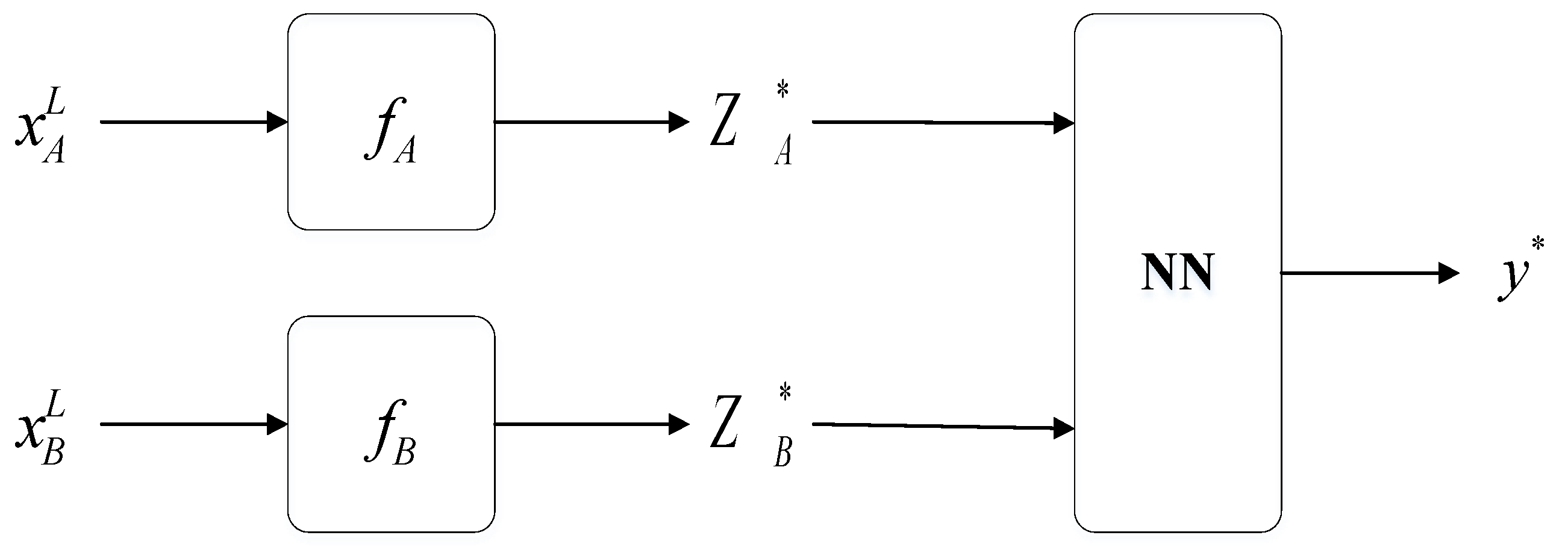
First, it is proposed to train M1 [41] using data X, as shown in Figure 3. The corresponding hidden space of the labeled source data, x A and x B , is obtained through well-trained f A and f B for training the external classifier, i.e., the NN model. The external classification models may be SVM, neural network, etc.
Due to the “KL disappearance” problem, achieving satisfactory balance between possibility and KL divergence is difficult. This is because KL loss may be undesirably reduced to zero, although it is expected to remain with a small value. To resolve this problem, the M1 model was implemented using “KL cost annealing” or “ β VAE” [44], which includes 5a new KL divergence weight factor, β . The modified evidence lower bound ( E L B O ) function of β VAE is as follows:
E L B O = E q ϕ ( z | x ) [ log p θ ( x | z ) ] β D K L ( q ϕ ( z | x ) p ( z ) )
During training, β is controlled to gradually increase from 0 to 1. When β < 1 , the potential variable, z , is trained, with emphasis on capturing useful features for reconstructing the observed value, x . When β = 1 , the previously learned z can be considered a satisfactory initialization, enabling the decoders to use more informative potential features [45].
After training, the M1 model can balance its reconstructed and generated features, and the potential variable, Z, in potential space is used as the discriminant feature of the external classifier. The SVM classifier is used in this study, although any preferred classifier can be employed. The M1 model performs discriminative feature extraction and reduces the dimension of input data; this is expected to improve the performance of external classifiers. In this study, the input data dimension is 1024, which is reduced to 128 in potential space. The data used in this paper are the raw data. All the input dimensions mentioned in the text are array dimensions. In this paper, SVM is chosen because of its better performance and robustness against small sample problems, the method is less affected by kernel functions in some successful cases, and it has some information filtering ability.
Because VAE (i.e., f and h models) and the classifier g model are separately trained, some information may be lost during training, and only labeled data are used in the g model training. The insufficient amount of labeled data can lead to a long training time and inadequate model prediction accuracy after training.
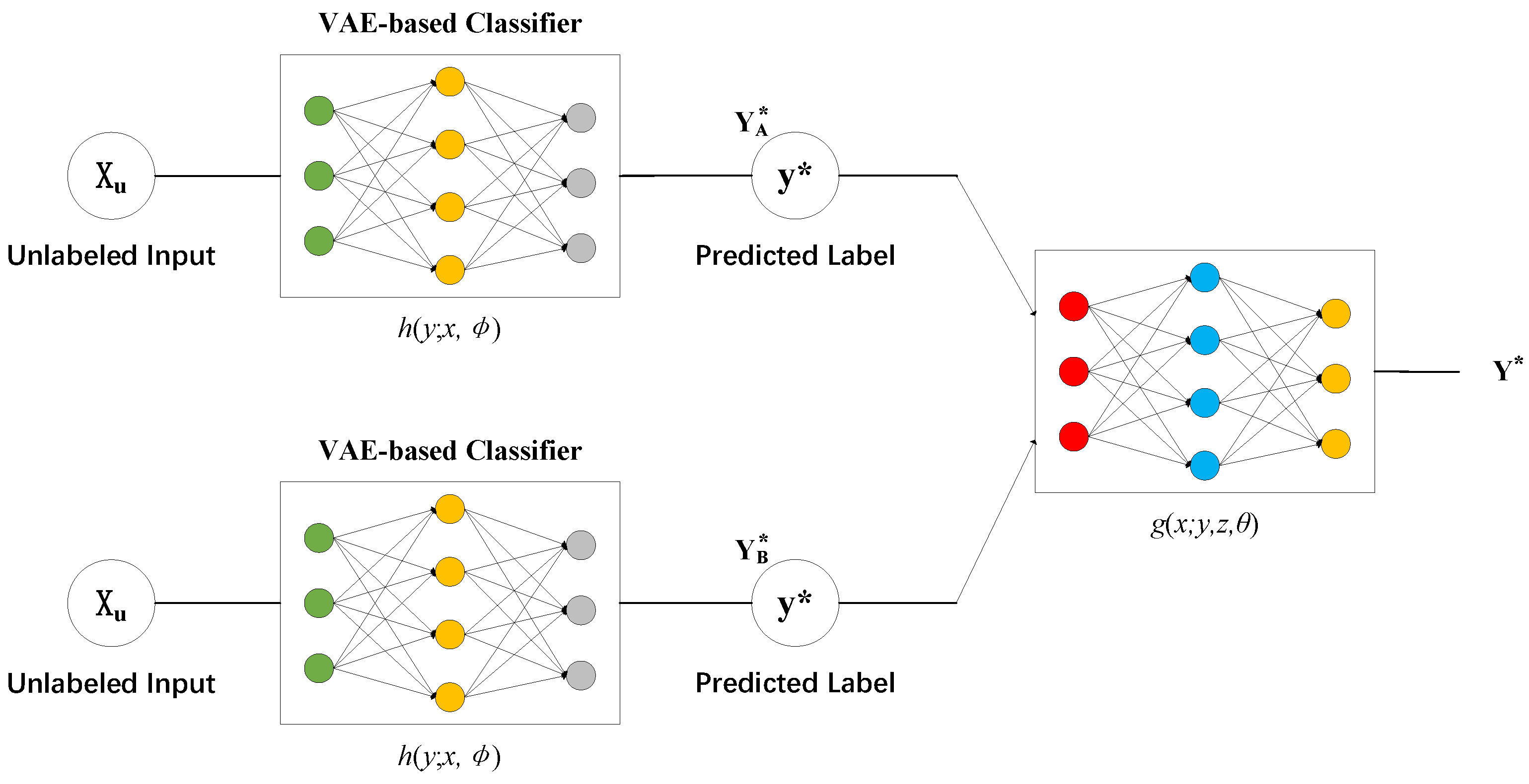
Considering the foregoing problems based on M1, the M2 model is proposed in this paper. Moreover, the VAE and its classifier models are trained simultaneously. The external classification model used here is also a neural network. Finally, the classifier result is fused by RF to obtain the final decision. The deep generation M2 model uses the same q ϕ ( z | x ) structure employed by the M1 model, and the decoder, p θ ( x | z ) , has the same setup as p θ ( x | z ) of M1. In addition, the classifier, q ϕ ( y | x ) , consists of two convolutional layers and two maximum pool layers, which contain loss and ReLU activation, followed by the final softmax layer. It is shown in Figure 4.
Two independent neural networks are used: one for labeled data and another for unlabeled data. Labeled and unlabeled data have the same network structure; however, they have different input/output specifications and loss functions. For example, for labeled data, x l and y are treated as inputs to minimize the ( x , y ) p ˜ l part in the labels in the formula, whereas the output is reconstructed as x l * and y * . For unlabeled data, x u is the only input; it is used for reconstructing x u .
The classifier and VAE are trained simultaneously; hence, their results are better than those reported in the literature [32]. However, the method employed here failed to train the classifier model by combining the two parts of data together to obtain y * directly. This was because it could result in considerable difficulty in training and slow convergence. Therefore, the prediction was made by implementing RF after independent training; the schematic of the proposed method is shown in Figure 5. Figure 6 shows the flow chart of the method proposed in this article.
It can be seen from Figure 6 that the method proposed in this article first undergoes the acquisition of the original signal, analyzes the original signal, prints the label, and divides the signal into a training set and a test set. Then, it is necessary to input the original signal into the VAE method and the RF method for training, verify the result and, finally, output the result.

4. Experimental Verification

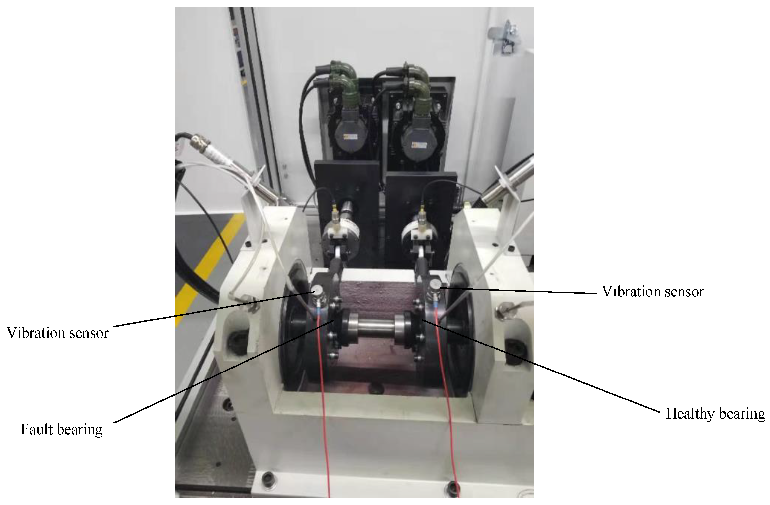
To validate the effectiveness of the proposed method, dynamic simulations were first performed to obtain theoretical computational data, which were then applied to VAERF as training data for deep learning. In this section, the effectiveness of two VAE-based semi-supervised depth generation models for bearing fault diagnosis is validated using a self-developed engineering experimental platform. The experimental method in this paper is based on the CWRU bearing experimental dataset [46]. The CWRU dataset is a public dataset; the experimental platform has a 2 hp motor drive, and the fault setting is a single point of failure that is set manually. The sampling frequency is 12 kHz or 48 kHz. The experimental sampling rate in this article is 48 kHz. The self-developed engineering experiment platform for fault signal acquisition and testing is described (Figure 7). The measurement of the speed signal of the rolling bearing differs from the measurement of the previous two signals in that it is obtained directly from the motor inverter. The system software uses the VISA standard configuration serial port to read the real-time speed of the bearing from the inverter via serial communication. In fact, the rotational frequency is read directly from the bearing and the bearing speed can be derived by conversion. Defective bearings, such as those with internal race failures, and working bearings were mounted on the test stand; the accelerometers were mounted in the vertical direction. The faulty bearing was mounted on the left side of the shaft, whereas the working bearing was mounted on the right side.
This section describes the developed diagnostic framework. It presents a comparison of the performance of the classifier with three baseline supervised/semi-supervised algorithms (PCA, AE and CNN). Then, the proposed approach is compared with some state-of-the-art semi-supervised learning algorithms, such as low-density separation [47] and secure semi-supervised SVM [48].
For the use of raw data, the diagnostic process starts with data segmentation, where the acquired signals are divided into multiple segments of equal length. The number of data samples of the drive-side vibration signal for each bearing failure is approximately 120,000 at three different speeds (i.e., 1730, 1750, and 1772 rpm). The data collected at these speeds constitute the complete data for each category, which will later be segmented using a fixed window size of 1024 samples and a sliding rate of 0.2 for the segmentation. Finally, the number of training and test data segments is 12,900 and 900, respectively. All test data are labeled. Although the percentage of test data seems small at first glance, at most, 2150 training data segments are labeled in the later experiments, which indicates that the percentage of test data over labeled training data is about 30%. After the initial data import and segmentation phase, these data segments remained in the order of their class labels or fault types. Therefore, data reorganization is required to ensure that both the training and test sets represent the overall distribution of the data, thus further improving model generalization and reducing the possibility of overfitting. Classical normalization techniques are also applied to the training and test sets to ensure that the vibration data have zero mean and unit variance, which is achieved by subtracting the mean of the original data and then dividing it by its standard deviation.
The network structure of VAE-based deep generation M1 and M2 models is discussed in detail in Section 3. In addition to implementing these bearing fault diagnosis models, other popular unsupervised learning schemes, such as PCA and AE are also trained as baselines. Their parameters are either selected to be consistent with the M1 and M2 models or obtained by parameter adjustment. This experiment is trained 100 times, and the batch size is set to 200. Specifically, the baseline of the method proposed in this article has two convolution layers with ReLU activation, each with 3 × 3 convolutions and 32 filters, followed by a 2 × 2 max-pooling layer and a 0.25 dropout layer. For example, the same optimizer setup as that of the VAE model (RMSprop) (with an initial learning rate of 10−4) was employed to train AE benchmarks. Details are as follows:
(1)
PCA-SVM: The PCA-SVM benchmark was trained using low-dimensional features extracted from labeled data segments (each data segment consists of 1024 data samples). The feature space dimension was 128, which is consistent with the dimensions of the potential space of M1 and M2 models. It supports the SVM in using the radial basis function kernel; its regularization parameter was set as C = 10 . Moreover, the kernel coefficient was set to “sample” ( 1 / 128 / X . var ( ) ), where X . var ( ) is the input data variance. This method first performed PCA cluster analysis on the original data, and then performed SVM classification.
(2)
AE: The AE structure is similar to that of VAE; hence, the AE baseline inherits the same network structure (encoder–decoder) as those of the M1 and SVM-based external classifiers.
(3)
CNN: the CNN benchmark treats each data segment of the time-series vibration (consisting of 1024 data samples) as a 2-D 32 × 32 image, in which it is a common practice to apply the vanilla CNN on bearing fault diagnosis. Specifically, the CNN baseline has two ReLU activation of convolution layers, each one has 2 × 2 convolutions and 32 filters, and a 2 × 2 max-pooling layer and a 0.25 dropout layer, respectively. In addition, we also set up a fully connected hidden layer with dimension 512, and its output is used as the input of softmax layer. At the same time, we use the cross entropy loss method and use the empirical value to set the batch to 10.
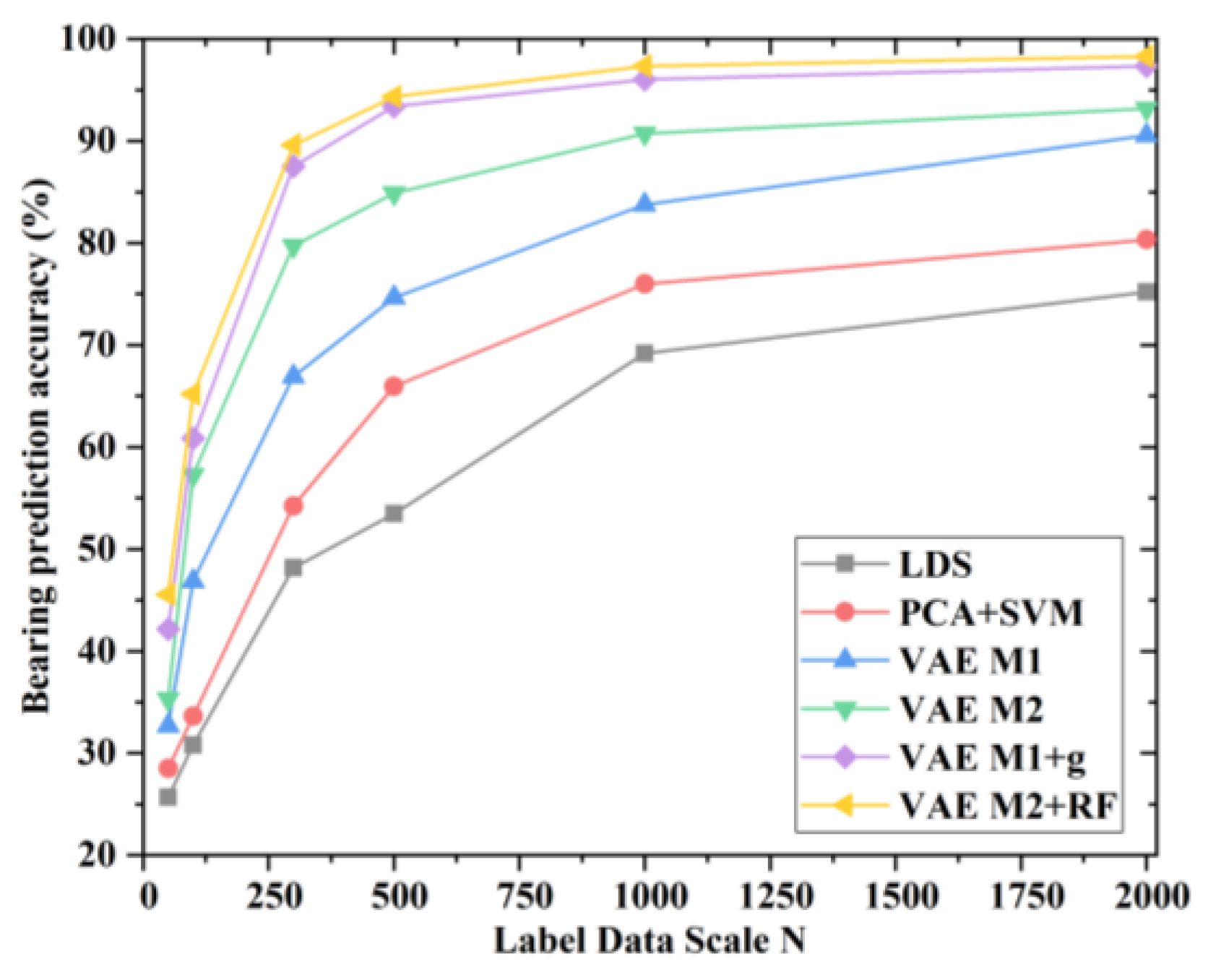
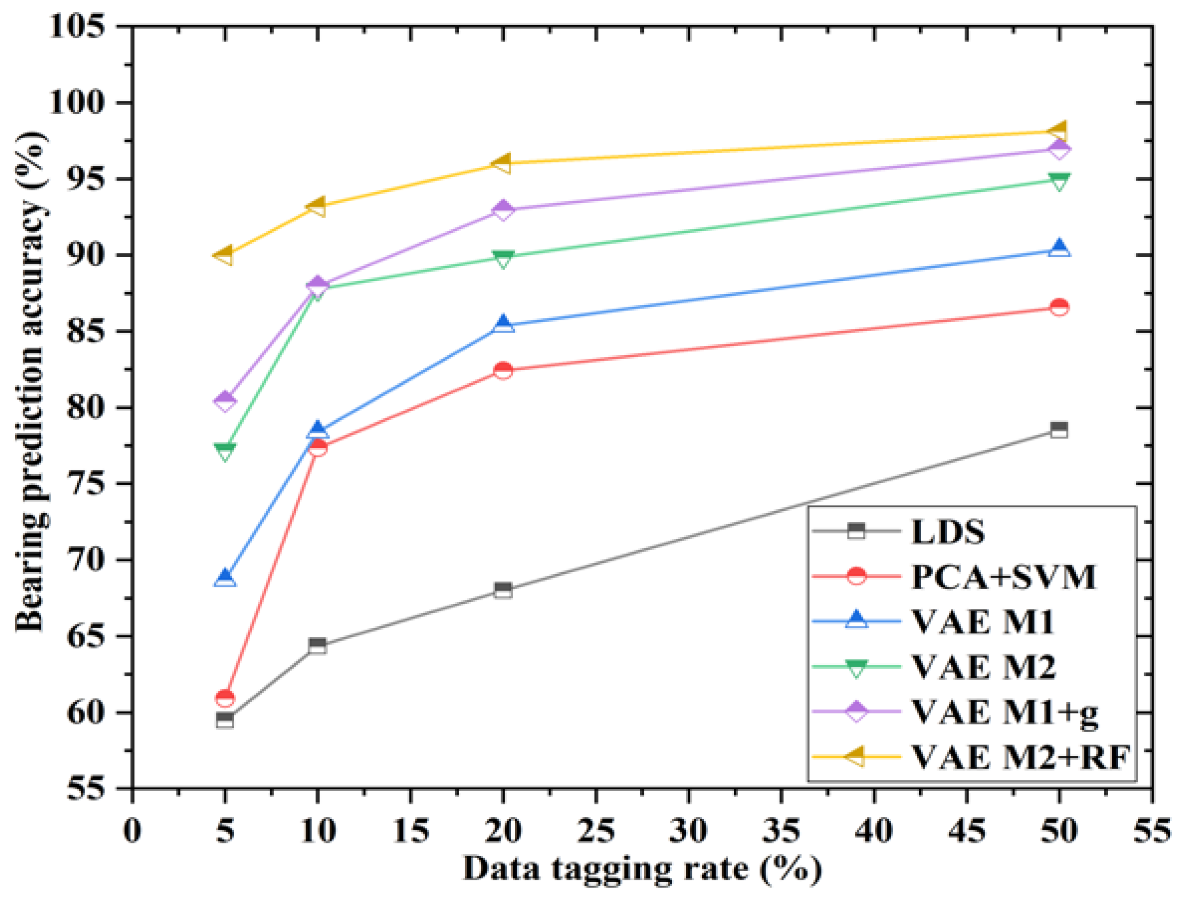
This can be seen in Table 1 and Table 2. The bearing prediction datasets were used in the same randomly rearranged training and test sets. The average precision and standard deviation of the different algorithms after ten rounds of experiments are presented in the Table. The number of initial records was 11,300, which were divided into 10,170 training sets and 1130 test sets. Predictions were then made using the M1 VAE M1 + NN model and the M2 VAE M2 + RF model; the results are summarized in Table 2 below. Only a small number of labels are actually used for different algorithms to construct bearing fault classifiers. The list indicates that 0.49, 0.98, 2.95, 4.92, 9.83, and 19.67% of the training data had labels. When the label rates are 20% and with increasing label data size (N), several algorithms are used to generate predictions, and accurate values are obtained. In the current scale, with the increase in label probability, several algorithms were used for prediction; their accuracy is described below. Ten cases were studied by labeling the last 40, 100, 200, 400, 800, 1000, 2000, 4000, and 8000 data segments of the training set. Accuracy is the most common evaluation metric we use and is easily understood as the number of samples that are scored correctly divided by the number of all samples. Generally speaking, the higher the correct rate, the better the classifier. These data segments account for 0.49, 0.98, 2.95, 4.92, 9.83 and 19.67% of the training data. Table 1 summarizes the classification results after ten rounds of experiments. The performance of M1 was better than that of PCA but virtually the same as that of VAE. This indicates that the discriminant feature space of VAE has no distinct advantage over the coding space of the ordinary AE.
However, the performance of M1 was better than that of the supervised learning algorithm, CNN. By incorporating most of the unlabeled data into the training process (i.e., when the number of labeled data segments varied from N = 50 to N = 1000), the improvement rate was approximately 5–15%, and the standard deviation was considerably smaller. Similar to the comparison results listed in Table 2, the performance of the VAE-based M2 model was superior to the other four algorithms. This shows the advantage of combining the VAE training process with its built-in classifier. When the number of labeled training data increases from N = 1000 to N = 2000, critical values can be obtained, and the loss of the semi-supervised VAE M2 model is 3%.
It can be seen in Figure 8 and Figure 9 that the performance of the unsupervised learning algorithm without using data labels remains unchanged during training. This can be attributed to the fact that many of the correct data samples were mislabeled as false data. This also creates a problem because the use of insufficient data or considerable amounts of data with inaccurate labels compromises the accuracy of the classifier. Specifically, when N = 1000 and N = 2000, the best accuracy rates achieved by the three baseline algorithms were 75.83 and 80.40%, respectively, whereas the average accuracy rates of the VAE-based M2 model were 97.49 and 98.22%, respectively. This means that the use of a considerable amount of unlabeled data can effectively improve the performance of the classifier of the VAE-based semi-supervised deep generation model (especially the M2 model). In addition, the results also show that inaccurate labeling can reduce the accuracy of the supervised learning algorithm. Other hyperparameters of the M2 model are also selected empirically. For training, 200 batches of data were used; the latent variable dimension was 128. To set the optimal value, RMSprop was employed with the initial learning rate of 10 4 . Figure 10 shows the comparison of the accuracy of different methods. It can be seen from Figure 10 that the method proposed in this paper converged the fastest. Therefore, in the diagnosis of bearing faults with natural evolution in practical applications, the semi-supervised learning method is applicable. The data cost of this method is low, and data can be freely labeled while retaining more amounts of unlabeled data.

5. Conclusions

In this paper, to address the problem that weak magnetic signals, vibration and temperature signals are not studied in the field of information fusion, a semi-supervised depth generation model using two VAE-based models with RF models is proposed to achieve bearing fault diagnosis in the case of limited labeling. The proposed method lays the foundation for subsequent research on the analysis of bearing-life evolution.
In this paper, the results from the datasets from self-built experimental platforms show that the M2RF model can greatly outperform the baseline supervised and unsupervised learning algorithms; its advantage can reach 40.92% when only 4.92% of the training data are labeled. In addition, the VAE-based RF model has an advantage over the four advanced semi-supervised learning methods. The study validated the performance of two VAE-based semi-supervised depth generation models using experimental platform datasets. The results show that incorrect labeling degrades the performance of the classifiers of the mainstream supervised learning algorithm. Furthermore, using a semi-supervised depth generation model and keeping uncertain data unlabeled is an effective way to alleviate the above problem.
The proposed method in this paper still needs to be investigated on the issue of feature parameter selection, and only raw signals have been selected so far. The future research direction of the method is to combine it with different evaluation models to achieve the analysis of bearing-life evolution. Moreover, it is necessary to use fuzzy logic theory or confusion matrix in information fusion in order to realize the purpose of life evolution analysis and to study the parameter optimization problem of the method in depth.

Author Contributions

Conceptualization, J.M.; methodology, J.M.; software, G.Z.; validation, J.M.; investigation, J.M.; resources, C.L.; data curation, J.M.; writing—original draft preparation, J.M.; writing—review and editing, C.L.; visualization, C.L.; supervision, C.L.; project administration, C.L. All authors have read and agreed to the published version of the manuscript.

Funding

This research received no external funding.

Institutional Review Board Statement

Not applicable.

Informed Consent Statement

Not applicable.

Conflicts of Interest

The authors declare no conflict of interest.

References

  1. Rai, A.; Upadhyay, S.H. A review on signal processing techniques utilized in the fault diagnosis of rolling element bearings. Tribol. Int. 2016, 96, 289–306. [Google Scholar] [CrossRef]
  2. Li, Y.; Yang, Y.; Wang, X.; Liu, B.; Liang, X. Early fault diagnosis of rolling bearings based on hierarchical symbol dynamic entropy and binary tree support vector machine. J. Sound Vib. 2018, 428, 72–86. [Google Scholar] [CrossRef]
  3. Wang, Y.; Tang, B.; Qin, Y.; Huang, T. Rolling bearing fault detection of civil aircraft engine based on adaptive estimation of instantaneous angular speed. IEEE Trans. Ind. Inform. 2020, 16, 4938–4948. [Google Scholar] [CrossRef]
  4. Li, H.; Liu, T.; Wu, X.; Chen, Q. Research on bearing fault feature extraction based on singular value decomposition and optimized frequency band entropy. Mech. Syst. Signal Process. 2019, 118, 477–502. [Google Scholar] [CrossRef]
  5. Ma, J.; Zhan, L.; Li, C.; Li, Z. An improved intrinsic time-scale decomposition method based on adaptive noise and its application in bearing fault feature extraction. Meas. Sci. Technol. 2021, 32, 025103. [Google Scholar] [CrossRef]
  6. Hou, D.; Qi, H.; Luo, H.; Wang, C.; Yang, J. Comparative study on the use of acoustic emission and vibration analyses for the bearing fault diagnosis of high-speed trains. Struct. Health Monit. 2021, 2021, 14759217211036025. [Google Scholar] [CrossRef]
  7. Morales-Espejel, G. Thermal damage and fatigue estimation in heavily loaded lubricated rolling/sliding contacts with Micro-Geometry. Proc. Inst. Mech. Eng. Part J J. Eng. Tribol. 2021, 235, 1680–1691. [Google Scholar] [CrossRef]
  8. Xie, Z.; Zhu, W. An investigationn on the lubrication characteristics of floating ring bearing with consideration of multi-coupling factors. Mech. Syst. Signal Process. 2022, 162, 108086. [Google Scholar] [CrossRef]
  9. Przysowa, R.; Rokicki, E.; Majewski, P. Optimized magnetic sensors to measure speed and position in adverse environments. In Proceedings of the IET & ISA 60th International Instrumentation Symposium, London, UK, 24–26 June 2014. [Google Scholar]
  10. Han, Q.K.; Li, X.L.; Chu, F.L. Skidding behavior of cylindrical roller bearings under time-variable load conditions. Int. J. Mech. Sci. 2018, 135, 203–214. [Google Scholar] [CrossRef]
  11. Selvaraj, A.; Marappan, R. Experimental analysis of factors influencing the cage slip in cylindrical roller bearing. Int. J. Adv. Manuf. Technol. 2011, 53, 635–644. [Google Scholar] [CrossRef]
  12. Hou, Y.; Wang, X. Development of an experimental system to measure the cage slip of cylindrical roller bearing. Struct. Health Monit. 2020, 19, 510–519. [Google Scholar] [CrossRef]
  13. Liu, Z.; Xu, C.; Li, M.; Wang, Q.; Liu, H. Study on the rotational speed of bearing cage based on ultrasonic measurement. Porc. Imeche Part K J. Multi-Body Dyn. 2017, 231, 684–689. [Google Scholar]
  14. Tu, W.; Yu, W.; Shao, Y.; Yu, Y. A nonlinear dynamic vibration model of cylindrical roller bearing considering skidding. Nonlinear Dyn. 2021, 103, 2299–2313. [Google Scholar]
  15. Ma, J.; Zhuo, S.; Li, C.; Zhan, L.; Zhang, G. Study on Noncontact Aviation Bearing Faults and Speed Monitoring; IEEE: Piscataway, NJ, USA, 2021; pp. 1–21. [Google Scholar] [CrossRef]
  16. Gao, S.; Li, T.; Zhang, Y. Rolling bearing fault diagnosis of PSO–LSSVM based on CEEMD entropy fusion. Trans. Can. Soc. Mech. Eng. 2020, 44, 405–418. [Google Scholar] [CrossRef]
  17. Hoang, D.T.; Tran, X.T.; Van, M.; Kang, H.J. A Deep Neural Network-Based Feature Fusion for Bearing Fault Diagnosis. Sensors 2021, 21, 244. [Google Scholar] [CrossRef]
  18. Jiao, J.; Yue, J.; Pei, D. Multi-sensor information fusion method for vibration fault diagnosis of rolling bearing. In Proceedings of the 5th Asia Conference on Mechanical and Materials Engineering (ACMME 2017), Tokyo, Japan, 9–11 June 2017; Volume 241, p. 012034. [Google Scholar]
  19. Song, Q.; Zhao, S.; Wang, M. On the accuracy of fault diagnosis for rolling element bearings using improved DFA and multi-sensor data fusion method. Sensors 2020, 20, 6465. [Google Scholar] [CrossRef]
  20. Tang, X.; Gu, X.; Wang, J.; He, Q.; Zhang, F.; Lu, J. A bearing fault diagnosis method based on feature selection feedback network and improved DS evidence fusion. IEEE Access 2020, 8, 20523–20536. [Google Scholar] [CrossRef]
  21. Soualhi, A.; Taleb, S. Data fusion for fault severity estimation of ball bearings. In Proceedings of the 2018 IEEE International Conference on Industrial Technology, Lyon, France, 20–22 February 2018; pp. 2105–2110. [Google Scholar]
  22. Liu, Y.; Yan, X.; Zhang, C.; Liu, W. An ensemble convolutional neural networks for bearing fault diagnosis using multi-sensor data. Sensors 2019, 19, 5300. [Google Scholar] [CrossRef] [Green Version]
  23. Kamat, P.V.; Sugandhi, R.; Kumar, S. Deep learning-based anomaly-onset aware remaining useful life estimation of bearings. PeerJ Comput. Sci. 2021, 7, e795. [Google Scholar] [CrossRef]
  24. Sayyad, S.; Kumar, S.; Bongale, A.; Kamat, P.; Patil, S.; Kotecha, K. Data-Driven Remaining Useful Life Estimation for Milling Process: Sensors, Algorithms, Datasets, and Future Directions. IEEE Access 2021, 9, 110255–110286. [Google Scholar] [CrossRef]
  25. Safizadeh, M.S.; Latifi, S.K. Using multi-sensor data fusion for vibration fault diagnosis of rolling element bearings by accelerometer and load cell. Inf. Fusion 2014, 18, 1–8. [Google Scholar] [CrossRef]
  26. Safizadeh, M.S.; Golmohammadi, A. Ball bearing fault detection via multi-sensor data fusion with accelerometer and microphone. Insight Non-Destr. Test. Cond. Monit. 2021, 63, 168–175. [Google Scholar] [CrossRef]
  27. Li, Z.; Yan, X. Study on data fusion of multi-dimensional sensors for health monitoring of rolling bearings. Insight Non-Destr. Test. Cond. Monit. 2013, 55, 147–151. [Google Scholar] [CrossRef]
  28. Gunerkar, R.S.; Jalan, A.K. Classification of ball bearing faults using vibro-acoustic sensor data fusion. Exp. Tech. 2019, 43, 635–643. [Google Scholar] [CrossRef]
  29. Wang, X.; Mao, D.; Li, X. Bearing fault diagnosis based on vibro-acoustic data fusion and 1D-CNN network. Measurement 2021, 173, 108518. [Google Scholar] [CrossRef]
  30. Mostafa, S.A.; Mustapha, A.; Hazeem, A.A.; Khaleefah, S.H.; Mohammed, M.A. An Agent-Based Inference Engine for Efficient and Reliable Automated Car Failure Diagnosis Assistance. IEEE Access 2018, 6, 8322–8331. [Google Scholar] [CrossRef]
  31. Mohammed, M.A.; Abd Ghani, M.K.; Arunkumar, N.A.; Obaid, O.I.; Mostafa, S.A.; Jaber, M.M.; Burhanuddin, M.A.; Matar, B.M.; Ibrahim, D.A. Genetic case-based reasoning for improved mobile phone faults diagnosis. Comput. Electr. Eng. 2018, 71, 212–222. [Google Scholar] [CrossRef]
  32. Zhang, S.; Ye, F.; Wang, B.; Habetler, T.G. Semi-supervised bearing fault diagnosis and classification using variational autoencoder-based deep generative models. IEEE Sens. J. 2021, 21, 6476–6486. [Google Scholar] [CrossRef]
  33. Chen, Y.; Zaki, M.J. Kate: K-competitive autoencoder for text. In Proceedings of the 23rd ACM SIGKDD International Conference on Knowledge Discovery and Data Mining, Halifax, NS, Canada, 13–17 August 2017; pp. 85–94. [Google Scholar]
  34. Kingma, P.; Welling, M. Max welling. Auto-encoding variational bayes. In Proceedings of the 26th ACM Sigspatial International Conference on Advances in Geographic Information Systems, Seattle, WA, USA, 6–9 November 2018; pp. 973–978. [Google Scholar]
  35. Hershey, J.R.; Olesen, P.A. Approximating the Kullback Leibler divergence between Gaussian mixture models. In Proceedings of the IEEE International Conference on Acoustics Speech and Signal Processing, Honolulu, HI, USA, 15–21 April 2007; p. 317. [Google Scholar]
  36. Jiang, M.; Beutel, A.; Cui, P.; Hooi, B.; Yang, S.; Faloutsos, C. A general suspiciousness metric for dense blocks in multimodal data. In Proceedings of the IEEE International Conference on Data Mining, Atlantic City, NJ, USA, 14–17 November 2015; pp. 781–786. [Google Scholar]
  37. Van Engelen, J.E.; Hoos, H.H. A survey on semi-supervised learning. Mach. Learn. 2020, 109, 373–440. [Google Scholar] [CrossRef] [Green Version]
  38. Lahouar, A.; Slama, J.B.H. Hour-ahead wind power forecast based on random forests. Renew. Energy 2017, 109, 529–541. [Google Scholar] [CrossRef]
  39. Zhang, K.; Wang, Z.N.; Bai, X.T.; Shi, H.T.; Wang, Q. Effect of preload on the dynamic characteristics of ceramic bearings based on a dynamic thermal coupling model. Adv. Mech. Eng. 2020, 12, 1687814020903851. [Google Scholar] [CrossRef] [Green Version]
  40. Schmidhuber, J. Deep learning in neural networks: An overview. Neural Netw. 2015, 61, 85–117. [Google Scholar] [CrossRef] [Green Version]
  41. Shao, L.; Wu, D.; Li, X. Learning deep and wide: A spectral method for learning deep networks. IEEE Trans. Neural Netw. Learn. Syst. 2014, 25, 2303–2308. [Google Scholar] [CrossRef]
  42. Bordoloi, D.J.; Tiwari, R. Optimum multi-fault classification of gears with integration of evolutionary and SVM algorithms. Mech. Mach. Theory 2014, 73, 49–60. [Google Scholar] [CrossRef]
  43. Lee, J.; Qiu, H.; Yu, G.; Lin, J. Rexnord Technical Services, IMS, University of Cincinnati. Bearing Data Set, NASA Ames Prognostics Data Repository; NASA Ames Research Center: Moffett Field, CA, USA, 2017.
  44. Burgess, C.P.; Higgins, I.; Pal, A.; Matthey, L.; Watters, N.; Desjardins, G.; Lerchner, A. Understanding disentangling in β-VAE. arXiv 2018, arXiv:1804.03599. [Google Scholar]
  45. Fu, H.; Li, C.; Liu, X.; Gao, J.; Celikyilmaz, A.; Carin, L. Cyclical annealing schedule: A simple approach to mitigating KL vanishing. arXiv 2019, arXiv:1903.10145.2019. [Google Scholar]
  46. Case Western Reserve University Bearing Data Center Website [EB/OL]. 2011. Available online: http://csegroups.case.edu/bearingdatacenter/pages/download-data-file (accessed on 16 December 2020).
  47. Chapelle, O.; Zien, A. Semi-Supervised Classification by Low Density Separation. In Proceedings of the International Workshop on Artificial Intelligence and Statistics (AISTATS), Bridgetown, Barbados, 6–8 January 2005; pp. 57–64. [Google Scholar]
  48. Li, Y.-F.; Zhou, Z.-H. Towards making unlabeled data never hurt. IEEE Trans. Pattern Anal. Mach. Intell. 2015, 37, 175–188. [Google Scholar]
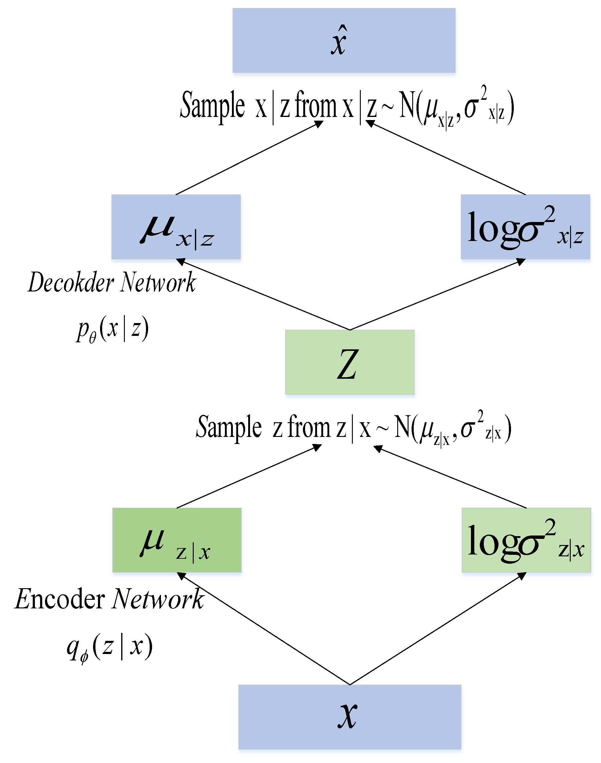
Figure 1. VAE network diagram.
Symmetry 14 00013 g001
Figure 2. Flowchart of the random forest algorithm.
Symmetry 14 00013 g002
Figure 3. M1 learning model.
Symmetry 14 00013 g003
Figure 4. Introduction of the semi-supervised generation M2 model.
Symmetry 14 00013 g004
Figure 5. Proposed semi-supervised generative method model.
Symmetry 14 00013 g005
Figure 6. Proposed method’s flow chart.
Symmetry 14 00013 g006
Figure 7. Experimental rig for real measurements.
Symmetry 14 00013 g007
Figure 8. Relationship between label size and accuracy.
Symmetry 14 00013 g008
Figure 9. Relationship between label rate and accuracy.
Symmetry 14 00013 g009
Figure 10. Accuracy of different methods.
Symmetry 14 00013 g010
Table 1. Summary of label proportion and accuracy.
N5010030050010002000
Proportion of labeled data training0.49%0.98%2.95%4.92%9.83%19.67%
CNN25.74 ± 2.88%30.50 ± 2.16%48.28 ± 3.42%53.41 ± 2.74%69.07 ± 1.46%75.19 ± 0.99%
PCA + SVM28.57 ± 0.38%33.77 ± 2.81%54.43 ± 1.59%66.27 ± 2.21%75.83 ± 1.27%80.40 ± 1.47%
VAE M132.93 ± 2.01%46.91 ± 1.37%67.03 ± 1.22%75.06 ± 1.76%83.97 ± 1.40%90.59 ± 1.43%
VAE M235.57 ± 2.91%57.04 ± 3.57%79.63 ± 2.80%85.16 ± 1.66%90.86 ± 0.51%93.06 ± 0.88%
VAE M1 + NN41.85 ± 2.34%62.34 ± 2.37%88.12 ± 1.63%93.33 ± 2.55%96.25 ± 0.90%97.32 ± 1.12%
VAE M2 + RF45.66 ± 2.45%65.12 ± 2.36%89.53 ± 1.89%94.33 ± 1.35%97.49 ± 0.38%98.22 ± 0.26%
Table 2. Summary of label probability and accuracy.
Algorithma = 5%a = 10%a = 20%a = 50%Ranking
CNN59.60 ± 15.43%64.49 ± 13.72%67.90 ± 12.98%78.53 ± 15.34%6
PCA + SVM60.85 ± 12.54%77.52 ± 12.48%82.44 ± 8.18%86.55 ± 13.34%5
VAE M168.75 ± 7.75%78.53 ± 8.37%85.40 ± 7.08%90.36 ± 8.37%4
VAE M277.17 ± 7.18%87.82 ± 4.63%89.80 ± 0.47%94.95 ± 0.26%3
VAE M1 + NN80.51 ± 5.47%88.02 ± 5.57%92.91 ± 5.18%96.97 ± 4.91%2
VAE M2 + RF90.12 ± 6.64%93.17 ± 5.59%95.95 ± 0.44%98.19 ± 0.11%1
Publisher’s Note: MDPI stays neutral with regard to jurisdictional claims in published maps and institutional affiliations.