Group Theoretical Description of the Periodic System

Abstract

The group theoretical description of the periodic system of elements in the framework of the Rumer–Fet model is considered. We introduce the concept of a single quantum system, the generating core of which is an abstract $C^{*}$-algebra. It is shown that various concrete implementations of the operator algebra depend on the structure of the generators of the fundamental symmetry group attached to the energy operator. In the case of the generators of the complex shell of a group algebra of a conformal group, the spectrum of states of a single quantum system is given in the framework of the basic representation of the Rumer–Fet group, which leads to a group-theoretic interpretation of the Mendeleev’s periodic system of elements. A mass formula is introduced that allows giving the termwise mass splitting for the main multiplet of the Rumer–Fet group. The masses of elements of the Seaborg table (eight-periodic extension of the Mendeleev table) are calculated starting from the atomic number $Z=3$ and going to $Z=220$. The continuation of the Seaborg homology between lanthanides and actinides is established with the group of superactinides. A 10-periodic extension of the periodic table is introduced in the framework of the group-theoretic approach. The multiplet structure of the extended table’s periods is considered in detail. It is shown that the period lengths of the system of elements are determined by the structure of the basic representation of the Rumer–Fet group. The theoretical masses of the elements of 10th and 11th periods are calculated starting from $Z=221$ and going to to $Z=364$. The concept of hypertwistor is introduced.

1. Introduction

The year 2019 marks the 150th anniversary of the discovery of the periodic law of chemical elements by Dmitry Ivanovich Mendeleev. Mendeleev’s periodic table sheds light on a huge number of experimental facts and allows the prediction of the existence and basic properties of new, previously unknown elements. However, the reasons (more precisely, root causes) for periodicity, in particular, the reasons for the periodic recurrence of similar electronic configurations of atoms, are still not clear. Furthermore, the limits of applicability of the periodic law have not yet been delineated—the controversy regarding the specifics of the nuclear and electronic properties of the atoms of heavy elements continues.

The now generally accepted structure of the periodic system, based on the Bohr model, proceeds from the fact that the arrangement of elements in the system with increasing atomic numbers is uniquely determined by the individual features of the electronic structure of atoms described in the framework of one-electronic approximation (Hartree method), and directly reflects the energy sequence of atomic orbitals of s, p, d, f-shells populated by electrons with an increasing total number as the charge of the nucleus of the atom increases in accordance with the principle of minimum energy. However, this is only possible in the simplest version of Hartree approximation, but in the variant of the Hartree–Fock approximation, the total energy of an atom is not equal to the sum of orbital energies, and the electron configuration of an atom is determined by the minimum of its full energy. As noted in the book [1], the traditional interpretation of the structure of the periodic system on the basis of the sequence of filling of electronic, atomic orbitals in accordance with their relative energies ${\epsilon }_{nl}$ is very approximate and has, of course, a number of drawbacks and has narrow limits of applicability. There is no universal sequence of orbital energies ${\epsilon }_{nl}$; moreover, such a sequence does not completely determine the order of the atomic orbitals settling by electrons since it is necessary to take into account the configuration interactions (superposition of configurations in the multi-configuration approximation). Furthermore, of course, periodicity is not only and not completely the orbital-energy effect. The reason for the repetition of similar electronic configurations of atoms in their ground states escapes us, and within one-electronic approximation can hardly be revealed at all. Moreover, it is possible that the theory of periodicity, in general, awaits a fate somewhat reminiscent of the fate of the theory of planetary retrogressions in the Ptolemaic system after the creation of the Copernican system. It is quite possible that what we call the periodicity principle is the result of the non-spatial symmetries of the atom (permutation and dynamical symmetries).

In 1971, academician V.A. Fock in his work [2], put the main question for the doctrine of the principle of periodicity and the theory of the periodic system: “Do the properties of atoms and their constituent parts fit into the framework of purely spatial representations, or do we need to somehow expand the concepts of space and spatial symmetry to accommodate the inherent degrees of freedom of atoms and their constituent parts?” [2], p. 108. As is known, Bohr’s model in its original formulation uses quantum numbers relating to electrons in a field with spherical symmetry, which allowed Bohr to introduce the concept of closed electron shells and bring this concept closer to the periods of the Mendeleev’s table. Despite this success, the problem of explaining the periodic system was far from solved. Moreover, for all the depth and radicality of these new ideas, they still fit into the framework of conventional spatial representations. A further important step was associated with the discovery of the internal, not spatial, degree of freedom of the electron—spin, which is not a mechanical concept. The discovery of spin is closely related to the discovery of the Pauli principle, which was formulated before quantum mechanics as requiring that each orbit, characterized by certain quantum numbers, contains no more than two electrons. At the end of the article [2], Fock himself answers his own question: “Purely spatial degrees of freedom of the electron is not enough to describe the properties of the electron shell of the atom and need to go beyond purely spatial concepts to express the laws that underlie the periodic system. The new degree of freedom of the electron—its spin—allows us to describe the properties of physical systems that are alien to classical concepts. This internal degree of electron freedom is essential for the formulation of the properties of multi-electron systems, thus for the theoretical justification of the Mendeleev’s periodic system” [2], p. 116.

The group-theoretic method of studying the periodic system was independently proposed by several authors in the early 1970s. In 1971, an article by Rumer and Fet [3] was published on the relationship between the group $\mathbf{Spin}\left(4\right)$ and Mendeleev’s table. In 1972, Asim Barut published his research on the group structure of the periodic system [4,5]. Simultaneously with these publications, articles by Octavio Navaro and co-authors [6,7] on the Hamiltonian model of the periodic system appear. Already from the first works in this direction, two different approaches are clearly manifested. The Navaro method (atomic physics approach), further developed in the works of Ostrovsky and Demkov [8,9,10], by analogy with atomic physics, relies on the search of a Hamiltonian model. On the other hand, the Rumer–Fet-Barut method (elementary particle approach) relies on the analogy with groups of dynamic (internal) symmetries of elementary particle physics, such as $\mathrm{SU}\left(2\right)$ (isotopic spin), $\mathrm{SU}\left(3\right)$ and $\mathrm{SU}\left(6\right)$. An exhaustive historical overview of this topic is presented in the work of Thyssen and Ceulemans [11].

In this paper, we consider the group theoretical description of the periodic system in the framework of the Rumer–Fet model. Unlike Bohr’s model, in which spatial and internal (spin) symmetries are combined on the basis of a classical composite system borrowed from celestial mechanics, the Rumer–Fet group G describes non-spatial symmetries (it is obvious that the visual-spatial image used in Bohr’s model is a vestige of classical representations. Therefore, in the middle of the 19th century, numerous attempts were made to build mechanical models of electromagnetic phenomena; even Maxwell’s treatise contains a large number of mechanical analogies. As time has shown, all mechanical models of electromagnetism turned out to be nothing more than auxiliary scaffolding, which was later discarded as unnecessary). However, group G also contains the Lorentz group (rotation group of the Minkowski space-time) as a subgroup. Moreover, the Rumer–Fet model is entirely based on the mathematical apparatus of quantum mechanics and group theory without involving any classical analogies, such as the concept of a composite system. The concept of a composite system, which directly follows from the principle of separability (the basic principle of reductionism), is known to have limited application in quantum mechanics, since in the microcosm, in contrast to the composite structure of the macrocosm, the superposition structure prevails. Heisenberg argued that the concept of “consists of” does not work in particle physics. On the other hand, the problem of “critical” elements of Bohr’s model is also a consequence of visual-spatial representations. Feynmann’s solution, representing the atomic nucleus as a point, leads to the Klein paradox for the element Uts (Untriseptium), with atomic number $Z=137$. Another spatial image, used in the Greiner–Reinhardt solution, represents the atomic nucleus as a charged ball, resulting in a loss of electroneutrality for atoms above the value $Z=173$ (see Section 4).

The most important characteristic feature of the Rumer–Fet model is the representation of the periodic table of elements as a single quantum system. While Bohr’s model considers an atom of one element as a separate quantum system (and the atomic number is included in the theory as a parameter, so that there are as many quantum systems as there are elements), in the Rumer–Fet model, atoms of various elements are considered as states of a single quantum system, connected to each other by the action of the symmetry group. A peculiar feature of the Rumer–Fet model is that it “ignores” the atomic structure underlying Bohr’s model. In contrast to Bohr’s model, which represents each atom as a composite aggregate of protons, neutrons and electrons, the Rumer–Fet model is distracted from the internal structure of every single atom, presenting the entire set of elements of the periodic table as a single quantum system of structureless states (the notion of the atom as a “structureless” state does not mean that there is no structure at all behind the concept. This only means that this structure is of a different order, not imported from the outside, from the “repertoire of classical physics”, but a structure that naturally follows from the mathematical apparatus of quantum mechanics (state vectors, symmetry group, Hilbert space, tensor products of Hilbert ($\mathbb{K}$-Hilbert) spaces and so on)). In this paper, the single quantum system $\mathbf{U}$ is defined by a $C^{*}$-algebra consisting of the energy operatorH and the generators of the fundamental symmetry group $G_f$ attached to H. The states of the system $\mathbf{U}$ are formed within the framework of the Gelfand–Naimark–Segal construction (GNS) [12,13]; that is, as cyclic representations of the operator algebra. Due to the generality of the task of the system $\mathbf{U}$ and the flexibility of the GNS-construction for each particular implementation of the operator algebra (the so-called “dressing” of the $C^{*}$-algebra), we obtain our (corresponding to this implementation) spectrum of states of the system $\mathbf{U}$ (thus, in the case when the generators of the fundamental symmetry group ($G_f={\mathrm{SO}}_0(1,3)$ is the Lorentz group) attached to H are generators of the complex shell of the group algebra $\mathfrak{sl}(2,\mathbb{C})$ (see Appendix A), we obtain a linearly growing spectrum of state masses (“elementary particles”) [14]. In this case, the “dressing” of the operator algebra and the construction of the cyclic representations of the GNS-construction are carried out in the framework of spinor structure (charged, neutral, truly neutral (Majorana) states and their discrete symmetries set through morphisms of the spinor structure, see [15,16,17,18,19,20]). In [14] it is shown that the masses of “elementary particles” are multiples of the mass of the electron with an accuracy of 0.41%. Here there is a direct analogy with the electric charge. Any electric charge is a multiple of the charge of the electron and a multiple of exactly. If any electric charge is absolutely a multiple of the electron charge, then in the case of masses, this multiplicity takes place with an accuracy of 0.41% (on average)). In Section 2 of this article, a conformal group is considered as a fundamental symmetry group ($G_f=\mathrm{SO}(2,4)$). In this case, the concrete implementation of the operator $C^{*}$-algebra is given by means of the generators of the complex shell of the group algebra $\mathfrak{so}(2,4)$ attached to H and the twistor structure associated with group $\mathrm{SU}(2,2)$ (the double covering of the conformal group). The complex shell of the algebra $\mathfrak{so}(2,4)$ leads to a representation $F_{s{s}^{\prime }}^{+}$ of the Rumer–Fet group, within which a group theoretical description of the periodic system of elements is given (Section 2). At this point, atoms are considered as states (discrete stationary states) of the matter spectrum (a term introduced by Heisenberg in the book [21] with reference to particle physics), each atom is given by a state vector of the physical Hilbert space, in which a symmetry group acts, translating some state vectors into others (that is, a group that specifies quantum transitions between elements of the periodic system). In Section 4, the Seaborg table (eight-periodic extension of the Mendeleev table) is formulated in the framework of the basic representation of the Rumer–Fet group for two different group chains, which specify the split of the main multiplet into smaller multiplets. It also calculates the average mass of the multiplets included in the Seaborg table (in addition to those multiplets that belong to the Mendeleev table with the exception of the elements Uue and Ubn). In Section 4 the mass formula is introduced to allow a termwise mass splitting for the basic representation of the Rumer–Fet group. The masses of elements are calculated starting from the atomic number $Z=3$ to $Z=220$ (except for the doublet containing hydrogen H and helium He). In Section 5 the 10-periodic extension of the Mendeleev table is studied. The multiplet structure of the extended table is considered in detail. It is shown that the period lengths of the system of elements are determined by the structure of the basic representation of the Rumer–Fet group. The theoretical masses of the elements of the 10th and 11th periods are calculated. In Section 6, quantum transitions between state vectors of the physical Hilbert space, formed by the set of elements of the periodic system, are considered.

It is possible to imagine an electron in any way: whether as a point (particle or wave), a charged ball or as an electron cloud on an atomic orbital, all these mental images only obscure the essence of the matter because they remain within the framework of visual-spatial representations. However, there is a mathematical structure that is far from visualization and yet accurately describes the electron: it is a two-component spinor, the vector of the fundamental representation of the double covering $\mathrm{SL}(2,\mathbb{C})\simeq {\mathbf{Spin}}_{+}(1,3)$ of the Lorentz group. Similarly, apart from any visual representations of the atom, it can be argued that the meaning is only the mathematical structure, which is directly derived from the symmetry group of the periodic system. In Section 7, it is shown that such structure is a hypertwistor acting in the $\mathbb{K}$-Hilbert space ${\mathbf{H}}_8\otimes {\mathbf{H}}_{\infty }$.

Bohr’s model does not explain the periodicity but only approximates it within the framework of one-electronic Hartree approximation. Apparently, the explanation of the periodic law lies on the path indicated by Fock; that it is necessary to go beyond the classical (space-time) representations in the description of the periodic system of elements. It is obvious that the most suitable scheme of description in this way is the group-theoretic approach.

2. Single Quantum System and Rumer–Fet Group

As already noted in the introduction, the starting point of the construction of the group theoretical description of the periodic system of elements is the concept of a single quantum system $\mathbf{U}$. Following Heisenberg, we assume that at the fundamental level, the definition of the system $\mathbf{U}$ is based on two concepts: energy and symmetry. Let us define a single quantum system $\mathbf{U}$ by means of the following axioms:

• A.I (Energy and fundamental symmetry) A single quantum system $\mathbf{U}$ at the fundamental level is characterized by a $C^{*}$-algebra $\mathfrak{A}$ with a unit consisting of the energy operator H and the generators of the fundamental symmetry group $G_f$ attached to H, forming a common system of eigenfunctions with H.
• A.II (States and GNS construction) The physical state of a $C^{*}$-algebra $\mathfrak{A}$ is determined by the cyclic vector $\left|\mathsf{\Phi }\right.⟩$ of the representation π of a $C^{*}$-algebra in a separable Hilbert space ${\mathsf{H}}_{\infty }$:

  $${\omega }_{\mathsf{\Phi }}\left(H\right)=\frac{⟨\mathsf{\Phi }\mid \pi \left(H\right)\mathsf{\Phi }⟩}{⟨\mathsf{\Phi }\mid \mathsf{\Phi }⟩}.$$
  The set $PS\left(\mathfrak{A}\right)$ of all pure states of a $C^{*}$-algebra $\mathfrak{A}$ coincides with the set of all states ${\omega }_{\mathsf{\Phi }}\left(H\right)$ associated with all irreducible cyclic representations π of an algebra $\mathfrak{A}$, $\left|\mathsf{\Phi }\right.⟩\in {\mathsf{H}}_{\infty }$ (Gelfand–Naimark–Segal construction).
• A.III (Physical Hilbert space) The set of all pure states ${\omega }_{\mathsf{\Phi }}\left(H\right)$ under the condition ${\omega }_{\mathsf{\Phi }}\left(H\right)\ge 0$ forms a physical Hilbert space ${\mathbf{H}}_{\mathrm{phys}}$ (in general, the space ${\mathbf{H}}_{\mathrm{phys}}$ is nonseparable). For each state vector $\left|\mathsf{\Psi }\right.⟩\in {\mathbf{H}}_{\mathrm{phys}}$ there is a unit ray $\mathbf{\Psi }=e^{i\alpha }\left|\mathsf{\Psi }\right.⟩$, where α runs through all real numbers and $\sqrt{⟨\mathsf{\Psi },\mid ,\mathsf{\Psi }⟩}=1$. The ray space is a quotient-space $\widehat{H}={\mathbf{H}}_{\mathrm{phys}}/S^1$, that is, the projective space of one-dimensional subspaces of ${\mathbf{H}}_{\mathrm{phys}}$. All states of a single quantum system $\mathbf{U}$ are described by the unit rays.
• A.IV (Axiom of spectrality) In $\widehat{H}$ there is a complete system of states with non-negative energy.
• A.V (Superposition principle) The basic correspondence between physical states and elements of space $\widehat{H}$ involves the superposition principle of quantum theory; that is, there is a set of basic states such that arbitrary states can be constructed from them using linear superpositions.

We choose a conformal group as the fundamental symmetry. The conformal group occurs in modern physics in a wide variety of situations and is essentially as universal as the Lorentz group; there are many relativistic theories and, similarly, conformal ones (moreover, as Segal showed [22], the Lie algebra of an inhomogeneous Lorentz group (that is, a Poincaré group) can be obtained by the deformation of a conformal Lie algebra. In turn, the conformal Lie algebra is “rigid”; that is, it cannot be obtained by deforming another Lie algebra. Because of this property, the conformal algebra (the algebra of a non-compact real pseudo-orthogonal group in a six-dimensional space with signature $(-,-,-,-,+,+)$) has a unique (complete) character and occupies a special place among other algebras).

2.1. Rumer–Fet Group

In the previous section, we defined a conformal group as the fundamental symmetry. The next logical step is to construct a concrete implementation of the operator algebra. We begin this construction by defining a complex shell of a group algebra $\mathfrak{so}(2,4)$ that leads to a basic representation $F_{s{s}^{\prime }}^{+}$ of the Rumer–Fet group (the first work in this direction is [3], where a striking similarity between the structure of the system of chemical elements and the structure of the energy spectrum of the hydrogen atom was noted. This similarity is explained in [3] within the framework of the Fock representation F [23] for group $\mathbf{Spin}\left(4\right)$ (the double covering of group $\mathrm{SO}\left(4\right)$). However, the main drawback of the description in [3] is the reducibility of the representation F, which did not allow the consideration of the system as “elementary” in the sense of group mechanics. In 1972, Konopelchenko [24] extended the Fock representation F to the representation $F^{+}$ of the conformal group, thus eliminating the above drawback. Further, based on the connection with the Madelung numbering, Fet defines the $F_s^{+}$ and $F_{s{s}^{\prime }}^{+}$ representations (to define the $F_{s{s}^{\prime }}^{+}$ representation, Madelung’s “lexicographic rule” had to be changed). After a rather long period of oblivion (totally undeserved), interest in the Rumer–Fet model will resume (see Kibler [25])).

As is known [26], a system of fifteen generators of the conformal group ${\mathrm{SO}}_0(2,4)$ satisfies the following commutativity relations:

$$\left[{\mathbf{L}}_{\alpha \beta },{\mathbf{L}}_{\gamma \delta }\right]=i\left(g_{\alpha \delta }{\mathbf{L}}_{\beta \gamma }+g_{\beta \gamma }{\mathbf{L}}_{\alpha \delta }-g_{\alpha \gamma }{\mathbf{L}}_{\beta \delta }-g_{\beta \delta }{\mathbf{L}}_{\alpha \gamma }\right),$$

$$(\alpha ,\beta ,\gamma ,\delta =1,\dots ,6,\alpha \ne \beta ,\gamma \ne \delta ).$$

Generators ${\mathbf{L}}_{\alpha \beta }$ form a basis of the group algebra $\mathfrak{so}(2,4)$. In order to move to the complex shell of the algebra $\mathfrak{so}(2,4)$, consider another system of generators proposed by Tsu Yao [26,27]. Let

$${\mathbf{J}}_1=1/2\left({\mathbf{L}}_{23}-{\mathbf{L}}_{14}\right),{\mathbf{J}}_2=1/2\left({\mathbf{L}}_{31}-{\mathbf{L}}_{24}\right),{\mathbf{J}}_3=1/2\left({\mathbf{L}}_{12}-{\mathbf{L}}_{34}\right),$$

$${\mathbf{K}}_1=1/2\left({\mathbf{L}}_{23}+{\mathbf{L}}_{14}\right),{\mathbf{K}}_2=1/2\left({\mathbf{L}}_{31}+{\mathbf{L}}_{24}\right),{\mathbf{K}}_3=1/2\left({\mathbf{L}}_{12}+{\mathbf{L}}_{34}\right),$$

$${\mathbf{P}}_1=1/2\left(-{\mathbf{L}}_{35}-{\mathbf{L}}_{16}\right),{\mathbf{P}}_2=1/2\left({\mathbf{L}}_{45}-{\mathbf{L}}_{36}\right),{\mathbf{P}}_0=1/2\left(-{\mathbf{L}}_{34}-{\mathbf{L}}_{56}\right),$$

$${\mathbf{Q}}_1=1/2\left({\mathbf{L}}_{35}-{\mathbf{L}}_{46}\right),{\mathbf{Q}}_2=1/2\left({\mathbf{L}}_{45}+{\mathbf{L}}_{36}\right),{\mathbf{Q}}_0=1/2\left({\mathbf{L}}_{34}-{\mathbf{L}}_{56}\right),$$

$${\mathbf{S}}_1=1/2\left(-{\mathbf{L}}_{15}+{\mathbf{L}}_{26}\right),{\mathbf{S}}_2=1/2\left(-{\mathbf{L}}_{25}-{\mathbf{L}}_{16}\right),{\mathbf{S}}_0=1/2\left({\mathbf{L}}_{12}-{\mathbf{L}}_{56}\right),$$

$${\mathbf{T}}_1=1/2\left(-{\mathbf{L}}_{15}-{\mathbf{L}}_{26}\right),{\mathbf{T}}_2=1/2\left({\mathbf{L}}_{25}-{\mathbf{L}}_{16}\right),{\mathbf{T}}_0=1/2\left(-{\mathbf{L}}_{12}-{\mathbf{L}}_{56}\right).$$

(1)

This system of eighteen generators is tied by the three relations

$${\mathbf{J}}_3-{\mathbf{K}}_3={\mathbf{P}}_0-{\mathbf{Q}}_0,{\mathbf{J}}_3+{\mathbf{K}}_3={\mathbf{S}}_0-{\mathbf{T}}_0,{\mathbf{P}}_0+{\mathbf{Q}}_0={\mathbf{S}}_0+{\mathbf{T}}_0.$$

(2)

In virtue of the independence of the generators ${\mathbf{L}}_{\alpha \beta }$ ($\alpha <\beta$), system (1) defines a surplus system of generators of ${\mathrm{SO}}_0(2,4)$, from which we can obtain the basis of $\mathfrak{so}(2,4)$, excluding three generators by means of (2).

Introducing the generators

$${\mathbf{J}}_{\pm }={\mathbf{J}}_1\pm i{\mathbf{J}}_2,{\mathbf{P}}_{\pm }={\mathbf{P}}_1\pm i{\mathbf{P}}_2,{\mathbf{S}}_{\pm }={\mathbf{S}}_1\pm i{\mathbf{S}}_2,$$

$${\mathbf{K}}_{\pm }={\mathbf{K}}_1\pm i{\mathbf{K}}_2,{\mathbf{Q}}_{\pm }={\mathbf{Q}}_1\pm i{\mathbf{Q}}_2,{\mathbf{T}}_{\pm }={\mathbf{T}}_1\pm i{\mathbf{T}}_2,$$

(3)

we come to the complex shell of the algebra $\mathfrak{so}(2,4)$.

Then

$$\left[{\mathbf{J}}_3,{\mathbf{J}}_{+}\right]={\mathbf{J}}_{+},\left[{\mathbf{J}}_3,{\mathbf{J}}_{-}\right]=-{\mathbf{J}}_{-},\left[{\mathbf{J}}_{+},{\mathbf{J}}_{-}\right]=2{\mathbf{J}}_3,$$

$$\left[{\mathbf{K}}_3,{\mathbf{K}}_{+}\right]={\mathbf{K}}_{+},\left[{\mathbf{K}}_3,{\mathbf{K}}_{-}\right]=-{\mathbf{K}}_{-},\left[{\mathbf{K}}_{+},{\mathbf{K}}_{-}\right]=2{\mathbf{K}}_3,$$

$$\left[{\mathbf{P}}_0,{\mathbf{P}}_{+}\right]={\mathbf{P}}_{+},\left[{\mathbf{P}}_0,{\mathbf{P}}_{-}\right]=-{\mathbf{P}}_{-},\left[{\mathbf{P}}_{+},{\mathbf{P}}_{-}\right]=-2{\mathbf{P}}_0,$$

$$\left[{\mathbf{Q}}_0,{\mathbf{Q}}_{+}\right]={\mathbf{Q}}_{+},\left[{\mathbf{Q}}_0,{\mathbf{Q}}_{-}\right]=-{\mathbf{Q}}_{-},\left[{\mathbf{Q}}_{+},{\mathbf{Q}}_{-}\right]=-2{\mathbf{Q}}_0,$$

$$\left[{\mathbf{S}}_0,{\mathbf{S}}_{+}\right]={\mathbf{S}}_{+},\left[{\mathbf{S}}_0,{\mathbf{S}}_{-}\right]=-{\mathbf{S}}_{-},\left[{\mathbf{S}}_{+},{\mathbf{S}}_{-}\right]=-2{\mathbf{S}}_0,$$

$$\left[{\mathbf{T}}_0,{\mathbf{T}}_{+}\right]={\mathbf{T}}_{+},\left[{\mathbf{T}}_0,{\mathbf{T}}_{-}\right]=-{\mathbf{T}}_{-},\left[{\mathbf{T}}_{+},{\mathbf{T}}_{-}\right]=-2{\mathbf{T}}_0,$$

$$\left[{\mathbf{J}}_i,{\mathbf{K}}_j\right]=0(i,j=+,-,3),$$

$$\left[{\mathbf{J}}_{+},{\mathbf{P}}_{+}\right]=0,\left[{\mathbf{J}}_{+},{\mathbf{P}}_{-}\right]=-{\mathbf{T}}_{-},\left[{\mathbf{J}}_{+},{\mathbf{P}}_0\right]=-1/2{\mathbf{J}}_{+},$$

$$\left[{\mathbf{J}}_{-},{\mathbf{P}}_{+}\right]={\mathbf{T}}_{+},\left[{\mathbf{J}}_{-},{\mathbf{P}}_{-}\right]=0,\left[{\mathbf{J}}_{-},{\mathbf{P}}_0\right]=1/2{\mathbf{J}}_{-},$$

$$\left[{\mathbf{J}}_3,{\mathbf{P}}_{+}\right]=1/2{\mathbf{P}}_{+},\left[{\mathbf{J}}_3,{\mathbf{P}}_{-}\right]=-1/2{\mathbf{P}}_{-},\left[{\mathbf{J}}_3,{\mathbf{P}}_0\right]=0,$$

$$\left[{\mathbf{J}}_{+},{\mathbf{Q}}_{+}\right]={\mathbf{S}}_{+},\left[{\mathbf{J}}_{+},{\mathbf{Q}}_{-}\right]=0,\left[{\mathbf{J}}_{+},{\mathbf{Q}}_0\right]=1/2{\mathbf{J}}_{+},$$

$$\left[{\mathbf{J}}_{-},{\mathbf{Q}}_{+}\right]=0,\left[{\mathbf{J}}_{-},{\mathbf{Q}}_{-}\right]=-{\mathbf{S}}_{-},\left[{\mathbf{J}}_{-},{\mathbf{Q}}_0\right]=-1/2{\mathbf{J}}_{-},$$

$$\left[{\mathbf{J}}_3,{\mathbf{Q}}_{+}\right]=-1/2{\mathbf{Q}}_{+},\left[{\mathbf{J}}_3,{\mathbf{Q}}_{-}\right]=1/2{\mathbf{Q}}_{-},\left[{\mathbf{J}}_3,{\mathbf{Q}}_0\right]=0,$$

$$\left[{\mathbf{J}}_{+},{\mathbf{S}}_{+}\right]=0,\left[{\mathbf{J}}_{+},{\mathbf{S}}_{-}\right]=-{\mathbf{Q}}_{-},\left[{\mathbf{J}}_{+},{\mathbf{S}}_0\right]=-1/2{\mathbf{J}}_{+},$$

$$\left[{\mathbf{J}}_{-},{\mathbf{S}}_{+}\right]={\mathbf{Q}}_{+},\left[{\mathbf{J}}_{-},{\mathbf{S}}_{-}\right]=0,\left[{\mathbf{J}}_{-},{\mathbf{S}}_0\right]=1/2{\mathbf{J}}_{-},$$

$$\left[{\mathbf{J}}_3,{\mathbf{S}}_{+}\right]=1/2{\mathbf{S}}_{+},\left[{\mathbf{J}}_3,{\mathbf{Q}}_{-}\right]=-1/2{\mathbf{S}}_{-},\left[{\mathbf{J}}_3,{\mathbf{S}}_0\right]=0,$$

$$\left[{\mathbf{J}}_{+},{\mathbf{T}}_{+}\right]={\mathbf{P}}_{+},\left[{\mathbf{J}}_{+},{\mathbf{T}}_{-}\right]=0,\left[{\mathbf{J}}_{+},{\mathbf{T}}_0\right]=1/2{\mathbf{J}}_{+},$$

$$\left[{\mathbf{J}}_{-},{\mathbf{T}}_{+}\right]=0,\left[{\mathbf{J}}_{-},{\mathbf{T}}_{-}\right]=-{\mathbf{P}}_{-},\left[{\mathbf{J}}_{-},{\mathbf{T}}_0\right]=-1/2{\mathbf{J}}_{-},$$

$$\left[{\mathbf{J}}_3,{\mathbf{T}}_{+}\right]=-1/2{\mathbf{T}}_{+},\left[{\mathbf{J}}_3,{\mathbf{T}}_{-}\right]=1/2{\mathbf{T}}_{-},\left[{\mathbf{J}}_3,{\mathbf{T}}_0\right]=0,$$

$$\left[{\mathbf{K}}_{+},{\mathbf{P}}_{+}\right]=-{\mathbf{S}}_{+},\left[{\mathbf{K}}_{+},{\mathbf{P}}_{-}\right]=0,\left[{\mathbf{K}}_{+},{\mathbf{P}}_0\right]=1/2{\mathbf{K}}_{+},$$

$$\left[{\mathbf{K}}_{-},{\mathbf{P}}_{+}\right]=0,\left[{\mathbf{K}}_{-},{\mathbf{P}}_{-}\right]={\mathbf{S}}_{-},\left[{\mathbf{K}}_{-},{\mathbf{P}}_0\right]=-1/2{\mathbf{K}}_{-},$$

$$\left[{\mathbf{K}}_3,{\mathbf{P}}_{+}\right]=-1/2{\mathbf{P}}_{+},\left[{\mathbf{K}}_3,{\mathbf{P}}_{-}\right]=1/2{\mathbf{P}}_{-},\left[{\mathbf{K}}_3,{\mathbf{P}}_0\right]=0,$$

$$\left[{\mathbf{K}}_{+},{\mathbf{Q}}_{+}\right]=0,\left[{\mathbf{K}}_{+},{\mathbf{Q}}_{-}\right]={\mathbf{T}}_{-},\left[{\mathbf{K}}_{+},{\mathbf{Q}}_0\right]=-1/2{\mathbf{K}}_{+},$$

$$\left[{\mathbf{K}}_{-},{\mathbf{Q}}_{+}\right]=-{\mathbf{T}}_{+},\left[{\mathbf{K}}_{-},{\mathbf{Q}}_{-}\right]=0,\left[{\mathbf{K}}_{-},{\mathbf{Q}}_0\right]=1/2{\mathbf{K}}_{-},$$

$$\left[{\mathbf{K}}_3,{\mathbf{Q}}_{+}\right]=1/2{\mathbf{Q}}_{+},\left[{\mathbf{K}}_3,{\mathbf{Q}}_{-}\right]=-1/2{\mathbf{Q}}_{-},\left[{\mathbf{K}}_3,{\mathbf{Q}}_0\right]=0,$$

$$\left[{\mathbf{K}}_{+},{\mathbf{S}}_{+}\right]=0,\left[{\mathbf{K}}_{+},{\mathbf{S}}_{-}\right]={\mathbf{P}}_{-},\left[{\mathbf{K}}_{+},{\mathbf{S}}_0\right]=-1/2{\mathbf{K}}_{+},$$

$$\left[{\mathbf{K}}_{-},{\mathbf{S}}_{+}\right]=-{\mathbf{P}}_{+},\left[{\mathbf{K}}_{-},{\mathbf{S}}_{-}\right]=0,\left[{\mathbf{K}}_{-},{\mathbf{S}}_0\right]=1/2{\mathbf{K}}_{-},$$

$$\left[{\mathbf{K}}_3,{\mathbf{S}}_{+}\right]=1/2{\mathbf{S}}_{+},\left[{\mathbf{K}}_3,{\mathbf{S}}_{-}\right]=-1/2{\mathbf{S}}_{-},\left[{\mathbf{K}}_3,{\mathbf{S}}_0\right]=0,$$

$$\left[{\mathbf{K}}_{+},{\mathbf{T}}_{+}\right]=-{\mathbf{Q}}_{+},\left[{\mathbf{K}}_{+},{\mathbf{T}}_{-}\right]=0,\left[{\mathbf{K}}_{+},{\mathbf{T}}_0\right]=1/2{\mathbf{K}}_{+},$$

$$\left[{\mathbf{K}}_{-},{\mathbf{T}}_{+}\right]=0,\left[{\mathbf{K}}_{-},{\mathbf{T}}_{-}\right]={\mathbf{Q}}_{-},\left[{\mathbf{K}}_{-},{\mathbf{T}}_0\right]=-1/2{\mathbf{K}}_{-},$$

$$\left[{\mathbf{K}}_3,{\mathbf{T}}_{+}\right]=-1/2{\mathbf{T}}_{+},\left[{\mathbf{K}}_3,{\mathbf{T}}_{-}\right]=1/2{\mathbf{T}}_{-},\left[{\mathbf{K}}_3,{\mathbf{T}}_0\right]=0,$$

$$\left[{\mathbf{P}}_i,{\mathbf{Q}}_j\right]=0(i,j=+,-,0),$$

$$\left[{\mathbf{P}}_{+},{\mathbf{S}}_{+}\right]=0,\left[{\mathbf{P}}_{+},{\mathbf{S}}_{-}\right]={\mathbf{K}}_{-},\left[{\mathbf{P}}_{+},{\mathbf{S}}_0\right]=-1/2{\mathbf{P}}_{+},$$

$$\left[{\mathbf{P}}_{-},{\mathbf{S}}_{+}\right]=-{\mathbf{K}}_{+},\left[{\mathbf{P}}_{-},{\mathbf{S}}_{-}\right]=0,\left[{\mathbf{P}}_{-},{\mathbf{S}}_0\right]=1/2{\mathbf{P}}_{-},$$

$$\left[{\mathbf{P}}_0,{\mathbf{S}}_{+}\right]=1/2{\mathbf{S}}_{+},\left[{\mathbf{P}}_0,{\mathbf{S}}_{-}\right]=-1/2{\mathbf{S}}_{-},\left[{\mathbf{P}}_0,{\mathbf{S}}_0\right]=0,$$

$$\left[{\mathbf{P}}_{+},{\mathbf{T}}_{+}\right]=0,\left[{\mathbf{P}}_{+},{\mathbf{T}}_{-}\right]=-{\mathbf{J}}_{+},\left[{\mathbf{P}}_{+},{\mathbf{T}}_0\right]=-1/2{\mathbf{P}}_{+},$$

$$\left[{\mathbf{P}}_{-},{\mathbf{T}}_{+}\right]={\mathbf{J}}_{-},\left[{\mathbf{P}}_{-},{\mathbf{T}}_{-}\right]=0,\left[{\mathbf{P}}_{-},{\mathbf{T}}_0\right]=1/2{\mathbf{P}}_{-},$$

$$\left[{\mathbf{P}}_0,{\mathbf{T}}_{+}\right]=1/2{\mathbf{T}}_{+},\left[{\mathbf{P}}_0,{\mathbf{T}}_{-}\right]=-1/2{\mathbf{T}}_{-},\left[{\mathbf{P}}_0,{\mathbf{T}}_0\right]=0,$$

$$\left[{\mathbf{Q}}_{+},{\mathbf{S}}_{+}\right]=0,\left[{\mathbf{Q}}_{+},{\mathbf{S}}_{-}\right]=-{\mathbf{J}}_{-},\left[{\mathbf{Q}}_{+},{\mathbf{S}}_0\right]=-1/2{\mathbf{Q}}_{+},$$

$$\left[{\mathbf{Q}}_{-},{\mathbf{S}}_{+}\right]={\mathbf{J}}_{+},\left[{\mathbf{Q}}_{-},{\mathbf{S}}_{-}\right]=0,\left[{\mathbf{Q}}_{-},{\mathbf{S}}_0\right]=1/2{\mathbf{Q}}_{-},$$

$$\left[{\mathbf{Q}}_0,{\mathbf{S}}_{+}\right]=1/2{\mathbf{S}}_{+},\left[{\mathbf{Q}}_0,{\mathbf{S}}_{-}\right]=-1/2{\mathbf{S}}_{-},\left[{\mathbf{Q}}_0,{\mathbf{S}}_0\right]=0,$$

$$\left[{\mathbf{Q}}_{+},{\mathbf{T}}_{+}\right]=0,\left[{\mathbf{Q}}_{+},{\mathbf{T}}_{-}\right]={\mathbf{K}}_{+},\left[{\mathbf{Q}}_{+},{\mathbf{T}}_0\right]=-1/2{\mathbf{Q}}_{+},$$

$$\left[{\mathbf{Q}}_{-},{\mathbf{T}}_{+}\right]=-{\mathbf{K}}_{-},\left[{\mathbf{Q}}_{-},{\mathbf{T}}_{-}\right]=0,\left[{\mathbf{Q}}_{-},{\mathbf{T}}_0\right]=1/2{\mathbf{Q}}_{-},$$

$$\left[{\mathbf{Q}}_0,{\mathbf{T}}_{+}\right]=1/2{\mathbf{T}}_{+},\left[{\mathbf{Q}}_0,{\mathbf{T}}_{-}\right]=-1/2{\mathbf{T}}_{-},\left[{\mathbf{Q}}_0,{\mathbf{T}}_0\right]=0,$$

$$\left[{\mathbf{S}}_i,{\mathbf{T}}_j\right]=0(i,j=+,-,0).$$

Let us consider a special representation of the conformal group ${\mathrm{SO}}_0(2,4)$, which is analogous to the van der Waerden representation (A5) for the Lorentz group ${\mathrm{SO}}_0(1,3)$ (see Appendix A). This local representation of ${\mathrm{SO}}_0(2,4)$ is related immediately to the Fock representation for group $\mathrm{SO}\left(4\right)$ (see Appendix B). In essence, this representation is an extension of the Fock representation for $\mathrm{SO}\left(4\right)$ to the unitary representation of the conformal group ${\mathrm{SO}}_0(2,4)$ in the Fock space $\mathfrak{F}$ by the basis (A7). Using generators (3) of the complex shell of the algebra $\mathfrak{so}(2,4)$, we obtain

$$\begin{array}{ccc}& & {\mathbf{J}}_{-}|j,\sigma ,\tau ⟩=\sqrt{(j+\sigma )(j-\sigma +1)}|j,\sigma -1,\tau ⟩,\hfill \\ & & {\mathbf{J}}_{+}|j,\sigma ,\tau ⟩=\sqrt{(j-\sigma )(j+\sigma +1)}|j,\sigma +1,\tau ⟩,\hfill \\ & & {\mathbf{J}}_3|j,\sigma ,\tau ⟩=\sigma |j,\sigma ,\tau ⟩,\hfill \\ & & {\mathbf{K}}_{-}|j,\sigma ,\tau ⟩=\sqrt{(j+\tau )(j-\tau +1)}|j,\sigma ,\tau -1⟩,\hfill \\ & & {\mathbf{K}}_{+}|j,\sigma ,\tau ⟩=\sqrt{(j-\tau )(j+\tau +1)}|j,\sigma ,\tau +1⟩,\hfill \\ & & {\mathbf{K}}_3|j,\sigma ,\tau ⟩=\tau |j,\sigma ,\tau ⟩,\hfill \end{array}$$

$$\begin{array}{ccc}& & {\mathbf{P}}_{-}|j,\sigma ,\tau ⟩=-i\sqrt{(j+\sigma )(j-\tau )}\left|j-\frac{1}{2},\sigma -\frac{1}{2},\tau +\frac{1}{2}\right.⟩,\hfill \\ & & {\mathbf{P}}_{+}|j,\sigma ,\tau ⟩=i\sqrt{(j-\tau +1)(j+\sigma +1)}\left|j+\frac{1}{2},\sigma +\frac{1}{2},\tau -\frac{1}{2}\right.⟩,\hfill \\ & & {\mathbf{P}}_0|j,\sigma ,\tau ⟩=\left(j+\frac{\sigma -\tau +1}{2}\right)\sigma \left|j,\sigma ,\tau \right.⟩,\hfill \\ & & {\mathbf{Q}}_{-}|j,\sigma ,\tau ⟩=i\sqrt{(j+\tau )(j-\sigma )}\left|j-\frac{1}{2},\sigma +\frac{1}{2},\tau -\frac{1}{2}\right.⟩,\hfill \\ & & {\mathbf{Q}}_{+}|j,\sigma ,\tau ⟩=-i\sqrt{(j-\sigma +1)(j+\tau +1)}\left|j+\frac{1}{2},\sigma -\frac{1}{2},\tau +\frac{1}{2}\right.⟩,\hfill \\ & & {\mathbf{Q}}_0|j,\sigma ,\tau ⟩=\left(j-\frac{\sigma -\tau -1}{2}\right)\left|j,\sigma ,\tau \right.⟩,\hfill \end{array}$$

(4)

$$\begin{array}{ccc}& & {\mathbf{S}}_{-}|j,\sigma ,\tau ⟩=i\sqrt{(j+\sigma )(j+\tau )}\left|j-\frac{1}{2},\sigma -\frac{1}{2},\tau -\frac{1}{2}\right.⟩,\hfill \\ & & {\mathbf{S}}_{+}|j,\sigma ,\tau ⟩=-i\sqrt{(j+\tau +1)(j+\sigma +1)}\left|j+\frac{1}{2},\sigma +\frac{1}{2},\tau +\frac{1}{2}\right.⟩,\hfill \\ & & {\mathbf{S}}_0|j,\sigma ,\tau ⟩=\left(j+\frac{\sigma +\tau +1}{2}\right)\sigma \left|j,\sigma ,\tau \right.⟩,\hfill \\ & & {\mathbf{T}}_{-}|j,\sigma ,\tau ⟩=-i\sqrt{(j-\tau )(j-\sigma )}\left|j-\frac{1}{2},\sigma +\frac{1}{2},\tau +\frac{1}{2}\right.⟩,\hfill \\ & & {\mathbf{T}}_{+}|j,\sigma ,\tau ⟩=i\sqrt{(j-\sigma +1)(j-\tau +1)}\left|j+\frac{1}{2},\sigma -\frac{1}{2},\tau -\frac{1}{2}\right.⟩,\hfill \\ & & {\mathbf{T}}_0|j,\sigma ,\tau ⟩=\left(j-\frac{\sigma +\tau -1}{2}\right)\left|j,\sigma ,\tau \right.⟩.\hfill \end{array}$$

Formula (4) defines a unitary representation of the conformal group ${\mathrm{SO}}_0(2,4)$ in the Fock space $\mathfrak{F}$. Formula (4) includes the formulas for ${\mathsf{J}}_k$, ${\mathsf{K}}_k$, giving representations of ${\mathsf{\Phi }}_n$ in subspaces ${\mathfrak{F}}_n$ (see (A6), where $j_1=j_2=j$) and thus the Fock representation $\mathsf{\Phi }$ on the subgroup $\mathrm{SO}\left(4\right)$. Moreover, if we restrict ${\mathrm{SO}}_0(2,4)$ to a subgroup ${\mathrm{SO}}_0(1,3)$ (Lorentz group), we obtain the van der Waerden representation (A5) given by the generators ${\mathsf{X}}_k$, ${\mathsf{Y}}_k$, which proves the similarity of the complex shells of the group algebras $\mathfrak{so}(2,4)$ and $\mathfrak{sl}(2,\mathbb{C})$. The representation, defined by (4), is called an extension $F^{+}$ of the Fock representation on the conformal group [26]. However, the representation $F^{+}$ is insufficient for the description of the periodic system of elements. With that end in view, it is necessary to include a fourth Madelung number s (which is analogous to spin) that leads to a group (the first “doubling”)

$$\mathrm{SO}(2,4)\otimes \mathrm{SU}\left(2\right).$$

(5)

A representation $F_s^{+}={\phi }_2\otimes F^{+}$ of the group (5), where ${\phi }_2$ is a unitary representation of group $\mathrm{SU}\left(2\right)$ in space $C\left(2\right)$, already satisfies this requirement (inclusion of the Madelung number s). A basis of the space ${\mathfrak{F}}^2=C\left(2\right)\otimes \mathfrak{F}$ of the representation $F_s^{+}$ has the form

$$\begin{array}{c}|n,l,m,s⟩,n=1,2,\dots ;l=0,1,\dots ,n-1;\hfill \\ \hfill m=-l,-l+1,\dots ,l-1,l;s=-1/2,1/2.\end{array}$$

(6)

Here n, l, m are quantum numbers of the conformal group.

Let ${\mathit{\tau }}_k$ be generators of the Lie algebra of $\mathrm{SU}\left(2\right)$; then a generator ${\mathit{\tau }}_3$ commutes with all of the generators of the subgroup $\mathrm{SO}(2,4)\otimes \mathbf{1}$. For that reason, generators ${\mathbf{R}}_0$, ${\mathbf{L}}^2$, ${\mathbf{J}}_3+{\mathbf{K}}_3$, ${\mathit{\tau }}_3$ commute with each other. Eigenvectors of the operators, representing these generators in the space ${\mathfrak{F}}^2$, have the form

$$\left|n,l,m,\frac{1}{2}\right.⟩=\left[\begin{array}{c}{\mathsf{\Psi }}_{nlm}^1\\ 0\end{array}\right],\left|n,l,m,-\frac{1}{2}\right.⟩=\left[\begin{array}{c}0\\ {\mathsf{\Psi }}_{nlm}^2\end{array}\right]$$

with eigenvalues n, $l(l+1)$, m, $\frac{1}{2}$ and n, $l(l+1)$, m, $-\frac{1}{2}$. An action of the operators, representing generators ${\mathit{\tau }}_{+}$, ${\mathit{\tau }}_{-}$, ${\mathit{\tau }}_3$ in the space ${\mathfrak{F}}^2$, is defined by the following formulas:

$${\mathit{\tau }}_{+}\left|n,l,m,-\frac{1}{2}\right.⟩=\left|n,l,m,\frac{1}{2}\right.⟩,{\mathit{\tau }}_{-}\left|n,l,m,\frac{1}{2}\right.⟩=\left|n,l,m,-\frac{1}{2}\right.⟩,$$

$${\mathit{\tau }}_3\left|n,l,m,s\right.⟩=s\left|n,l,m,s\right.⟩.$$

In virtue of the Madelung numbering, the basis $\left|n,l,m,s\right.⟩$ stands in one-to-one correspondence with the elements of the periodic system. A relationship between the arrangement of the elements in the Mendeleev table and a number collection $(n,l,m,s)$ is defined by a so-called Madelung “lexicographic rule” $Z\leftrightarrow (n,l,m,s)$ (Erwin Madelung was the first to apply “hydrogen” quantum numbers n, l, m, s to the numbering of elements of the periodic table. It should be noted that the numbers n, l, m, s are not quantum numbers in Bohr’s model, because in this model, there is no single quantum-mechanical description of the system of elements, the latter is assigned an atomic number Z, distinguishing rather than combining individual quantum systems. The resulting classification of elements Madelung called “empirical” because he could not connect it with the Bohr model. Apparently, it was because of the lack of theoretical justification at the time (the 1920s), he published it as a reference material in [28]. Theoretical justification (understanding of the nature of Madelung numbers) was later given by Fet [26] from the position of group-theoretic vision. The history of Madelung numbers was also developed in a slightly different direction in the works of Kleczkowski [29], where the filling of the electronic levels of the atom was considered according to the rule of the sequential filling of $(n+l)$-groups (the so-called Madelung–Kleczkowski groups)):

(1)

elements are arranged in increasing order of atomic number Z;

(2)

collections $(n,l,m,s)$ are arranged in increasing order of $n+l$; at the given $n+l$ in increasing order of n; at the given $n+l$, n in increasing order of m; at the given $n+l$, n, m in increasing order of s;

(3)

the Z-th element corresponds to Z-th collection.

In Madelung numbering, the sum $n+l$ does not have a group sense: it is a sum of the quantum number n (an eigenvalue of the operator ${\mathbf{R}}_0=-{\mathbf{L}}_{56}$) and the number l, which is not a quantum number. In this case, a quantum number is $l(l+1)$ (an eigenvalue of the operator ${\mathbf{L}}^2={\mathbf{L}}_{12}^2+{\mathbf{L}}_{23}^2+{\mathbf{L}}_{31}^2$), and l only defines this quantum number. Therefore, in accordance with the group theoretical viewpoint, the number $n+l$ should be excluded from the formulation of the “lexicographic rule”. In [26], Fet introduced a new quantum number $\nu$, which is equal to $\nu =1/2(n+l+1)$ for the odd value of $n+l$ and $\nu =1/2(n+l)$ for the even value of $n+l$. The introduction of the quantum number $\nu$ allows us to change Madelung numbering, which leads to the following “lexicographic rule” (Fet rule):

(1)

the elements are arranged in increasing order of atomic number Z;

(2)

collections $(\nu ,\lambda ,\mu ,s,s^{\prime })$ are arranged in increasing order of $\nu$; at the given $\nu$ in increasing order of $s^{\prime }$; at the given $\nu$, $s^{\prime }$ in decreasing order of $\lambda$; at the given $\nu$, $s^{\prime }$, $\lambda$ in increasing order of $\mu$; at the given $\nu$, $s^{\prime }$, $\lambda$, $\mu$ in increasing order of s;

(3)

the Z-th element corresponds to Z-th collection.

The introduction of the fifth quantum number leads to another (second) “doubling” of the representation space. In this space, we have the Rumer–Fet group

$$\mathrm{SO}(2,4)\otimes \mathrm{SU}\left(2\right)\otimes \mathrm{SU}{\left(2\right)}^{\prime }.$$

(7)

A representation $F_{s{s}^{\prime }}^{+}={\phi }_2^{\prime }\otimes F_s^{+}$ of the group (7), where ${\phi }_2^{\prime }$ is a unitary representation of group $\mathrm{SU}{\left(2\right)}^{\prime }$ in the space $C\left(2\right)$, satisfies the requirement of inclusion of the fifth quantum number. A basis of the space ${\mathfrak{F}}^4=C\left(2\right)\otimes {\mathfrak{F}}^2$ of the representation $F_{s{s}^{\prime }}^{+}$ has the form

$$\begin{array}{c}|\nu ,\lambda ,\mu ,s,s^{\prime }⟩,\nu =1,2,\dots ;\lambda =0,1,\dots ,\nu -1;\hfill \\ \hfill \mu =-\lambda ,-\lambda +1,\dots ,\lambda -1,\lambda ;s=-1/2,1/2,s^{\prime }=-1/2,1/2.\end{array}$$

(8)

Let ${\mathit{\tau }}_k^{\prime }$ be generators of the Lie algebra $\mathrm{SU}{\left(2\right)}^{\prime }$; then the generator ${\mathit{\tau }}_3^{\prime }$ commutes with the all generators of the subgroup $\mathrm{SO}(2,4)\otimes \mathrm{SU}\left(2\right)\otimes \mathbf{1}$. Therefore, generators ${\mathbf{R}}_0=-{\mathbf{L}}_{56}={\mathbf{P}}_0+{\mathbf{Q}}_0={\mathbf{S}}_0+{\mathbf{T}}_0$, ${\mathbf{L}}^2$, ${\mathbf{J}}_3+{\mathbf{K}}_3$, ${\mathit{\tau }}_3$, ${\mathit{\tau }}_3^{\prime }$ commute with the each other. Common eigenvectors of the operators, which represent these generators in the space ${\mathfrak{F}}^4$, have the form

$$\left|\nu ,\lambda ,\mu ,s,+\frac{1}{2}\right.⟩=\left[\begin{array}{c}{\mathsf{\Psi }}_{\nu \lambda ,\mu }^1\\ {\mathsf{\Psi }}_{\nu \lambda ,\mu }^2\\ 0\\ 0\end{array}\right],\left|\nu ,\lambda ,\mu ,s,-\frac{1}{2}\right.⟩=\left[\begin{array}{c}0\\ 0\\ {\mathsf{\Psi }}_{\nu \lambda ,\mu }^3\\ {\mathsf{\Psi }}_{\nu \lambda ,\mu }^4\end{array}\right]$$

with eigenvalues $\nu$, $\lambda (\lambda +1)$, $\mu$, s, $\frac{1}{2}$ and $\nu$, $\lambda (\lambda +1)$, $\mu$, s, $-\frac{1}{2}$.

An action of the operators, representing the generators ${\mathit{\tau }}_{+}$, ${\mathit{\tau }}_{-}$, ${\mathit{\tau }}_3$ and ${\mathit{\tau }}_{+}^{\prime }$, ${\mathit{\tau }}_{-}^{\prime }$, ${\mathit{\tau }}_3^{\prime }$ in the space ${\mathfrak{F}}^4$, is defined by the following formulas:

$${\mathit{\tau }}_{+}\left|\nu ,\lambda ,\mu ,-\frac{1}{2},s^{\prime }\right.⟩=\left|\nu ,\lambda ,\mu ,\frac{1}{2},s^{\prime }\right.⟩,{\mathit{\tau }}_{-}\left|\nu ,\lambda ,\mu ,\frac{1}{2},s^{\prime }\right.⟩=\left|\nu ,\lambda ,\mu ,-\frac{1}{2},s^{\prime }\right.⟩,$$

$${\mathit{\tau }}_3\left|\nu ,\lambda ,\mu ,s,s^{\prime }\right.⟩=s\left|\nu ,\lambda ,\mu ,s,s^{\prime }\right.⟩.$$

$${\mathit{\tau }}_{+}^{\prime }\left|\nu ,\lambda ,\mu ,s,-\frac{1}{2}\right.⟩=\left|\nu ,\lambda ,\mu ,s,\frac{1}{2}\right.⟩,{\mathit{\tau }}_{-}^{\prime }\left|\nu ,\lambda ,\mu ,s,\frac{1}{2}\right.⟩=\left|\nu ,\lambda ,\mu ,s,-\frac{1}{2}\right.⟩,$$

$${\mathit{\tau }}_3^{\prime }\left|\nu ,\lambda ,\mu ,s,s^{\prime }\right.⟩=s^{\prime }\left|\nu ,\lambda ,\mu ,s,s^{\prime }\right.⟩.$$

The “addresses” of the elements (see Figure 1) are defined by a collection of quantum numbers of the Rumer–Fet group (7), which are numbering basis vectors $\left|\nu ,\lambda ,\mu ,s,s^{\prime }\right.⟩$ of the space ${\mathfrak{F}}^4$. Generators of the Lie algebra of $\mathrm{SO}(2,4)$ act on the quantum numbers $\nu$, $\lambda$, $\mu$ by means of formula (4), with a replacement of n, l, m via $\nu$, $\lambda$, $\mu$.

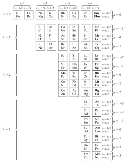
Figure 1. Mendeleev table in the form of the basic representation $F_{s{s}^{\prime }}^{+}$ of the Rumer–Fet group $\mathrm{SO}(2,4)\otimes \mathrm{SU}\left(2\right)\otimes \mathrm{SU}{\left(2\right)}^{\prime }$. The Periodic Table in this form first appeared in [3], with the exception of elements typed in bold.

There is the following chain of groups:

$$G\supset G_1\supset G_2⟼\mathrm{SO}(2,4)\otimes \mathrm{SU}\left(2\right)\otimes \mathrm{SU}\left(2\right)\supset \mathrm{SO}\left(4\right)\otimes \mathrm{SU}\left(2\right)\supset \mathrm{SO}\left(3\right)\otimes \mathrm{SU}\left(2\right).$$

(9)

The reduction of the basic representation $F_{s{s}^{\prime }}^{+}$ of the Rumer–Fet group on the subgroups is realized in accordance with the chain (9). Therefore, multiplets of a subgroup $\mathrm{SO}\left(3\right)\otimes \mathrm{SU}\left(2\right)$ are represented by vertical rectangles in Figure 1, and their elements compose well-known s, p, d and f-families (in particular, lanthanides and actinides are selected as multiplets of the subgroup $\mathrm{SO}\left(3\right)\otimes \mathrm{SU}\left(2\right)$). Each element occupies quite a definite place, which is defined by its “address” in the table $(\nu ,\lambda ,\mu ,s,s^{\prime })$; that is, by corresponding quantum numbers of the symmetry group. Thus, atoms of all possible elements stand in one-to-one correspondence with the vectors of the basis (8).

2.2. Mendeleev Table

In Figure 1, we mark the elements that had not yet been discovered or received their official names during the lifetimes of Rumer and Fet in bold script. These elements belong to the last column of Figure 1 with the quantum numbers $\nu =4$ and $s^{\prime }=1/2$: Db—Dubnium, Sg—Seaborgium, Bh—Bohrium, Hs—Hassium (eka-osmium), Mt—Meitnerium, Ds—Darmstadtium, Rg—Roentgenium, Cn—Copernicium (eka-mercury). All these elements belong to a multiplet with a quantum number $\lambda =2$. A multiplet with $\lambda =1$ ($\nu =4$, $s^{\prime }=1/2$) consists of recently discovered elements: Nh—Nihonium (eka-thallium), Fl—Flerovium (eka-lead), Mc—Moscovium (eka-bismuth), Lv—Livermorium (eka- polonium), Ts—Tennessine (eka-astatine), Og—Oganesson (eka-radon). Further, a multiplet with a quantum number $\lambda =0$ ($\nu =4$, $s^{\prime }=1/2$) is formed by undetected yet hypothetical elements, Uue—Ununennium (eka-francium), with a supposed atomic mass of 316 a.u. and Ubn—Unbinillium (eka-radium). All the enumerated elements accomplish the filling of the Mendeleev table (from the 1st to 120th number), inclusive of the value of quantum number $\nu =4$.

Let us calculate the masses of the hypothetical elements Uue and Ubn. Before we proceed, we calculate the average masses of the multiplets belonging to the Mendeleev table. With this aim in view, we use a mass formula proposed in [26]:

$$m=m_0+a\left[s^{\prime }(2\nu -3)-5\nu +\frac{11}{2}+2({\nu }^2-1)\right]-b·\lambda (\lambda +1),$$

(10)

where $m_0$, a, b are the coefficients that are underivable from the theory. This formula is analogous to a Gell-Mann–Okubo formula for the hadrons in $\mathrm{SU}\left(3\right)$-theory [30,31], and also to a Bég-Singh formula in $\mathrm{SU}\left(6\right)$-theory [32]. The formula (10) is analogous to the “first perturbation” in $\mathrm{SU}\left(3\right)$ and $\mathrm{SU}\left(6\right)$-theories, which allows the calculation of an average mass of the elements of the multiplet (an analog of the “second perturbation” for the Rumer–Fet group, which leads to the mass splitting inside the multiplet, we will give in Section 4). Table 1 contains the average masses of “heavy” multiplets ($\nu =3,4$) calculated according formula (10) at $m_0=1$, $a=17$, $b=5.5$. From Table 1, we see that an accuracy between experimental and theoretical masses rises with the growth of the “weight” of the multiplet; therefore, formula (10) is asymptotic. An exception is the last multiplet $(\nu =4,s^{\prime }=1/2,\lambda =0)$, consisting of the hypothetical elements Uue and Ubn, which have masses unconfirmed by experiments.

Table 1. Average masses of “heavy” multiplets.

	Multiplet	Mass (exp.)	Mass (theor.)	Approx. %
1.	$(\nu =3,s^{\prime }=-1/2,\lambda =2)$	$55.31$	53	$-4.36$
2.	$(\nu =3,s^{\prime }=-1/2,\lambda =1)$	$76.65$	75	$-2.2$
3.	$(\nu =3,s^{\prime }=-1/2,\lambda =0)$	$86.54$	86	$-0.63$
4.	$(\nu =3,s^{\prime }=1/2,\lambda =2)$	$99.76$	104	$4.07$
5.	$(\nu =3,s^{\prime }=1/2,\lambda =1)$	$123.51$	126	$1.98$
6.	$(\nu =3,s^{\prime }=1/2,\lambda =0)$	$135.12$	137	$1.37$
7.	$(\nu =4,s^{\prime }=-1/2,\lambda =3)$	$154.59$	156	$0.90$
8.	$(\nu =4,s^{\prime }=-1/2,\lambda =2)$	$187.96$	189	$0.55$
9.	$(\nu =4,s^{\prime }=-1/2,\lambda =1)$	$210.21$	211	$0.37$
10.	$(\nu =4,s^{\prime }=-1/2,\lambda =0)$	$224.52$	222	$-1.13$
11.	$(\nu =4,s^{\prime }=1/2,\lambda =3)$	$244.56$	241	$-1.48$
12.	$(\nu =4,s^{\prime }=1/2,\lambda =2)$	$273.10$	274	$0.33$
13.	$(\nu =4,s^{\prime }=1/2,\lambda =1)$	$290.83$	296	$1.75$
14.	$(\nu =4,s^{\prime }=1/2,\lambda =0)$	318 *	307	$-3.58$ *

3. Implementation of the Operator Algebra

As is known, in the foundation of an algebraic formulation of quantum theory, we have a Gelfand–Naimark–Segal (GNS) construction, which is defined by a canonical correspondence $\omega \leftrightarrow {\pi }_{\omega }$ between states and cyclic representations of the $C^{*}$-algebra [33,34,35].

Let us suppose that according to the axiom A.I (Section 2) generators of the conformal group (a fundamental symmetry $G_f=\mathrm{SO}(2,4)$ in this context) are attached to the energy operator H. Therefore, each eigensubspace ${\mathsf{H}}_E$ of the energy operator is invariant with respect to the operators of the representation $F^{+}$ of the conformal group (it follows from a similarity of the complex shells of the group algebras $\mathfrak{sl}(2,C)$, $\mathfrak{so}\left(4\right)$ and $\mathfrak{so}(2,4)$). It allows us to obtain a concrete implementation (“dressing”) of the operator algebra $\pi \left(\mathfrak{A}\right)\to \pi \left(H\right)$, where $\pi \equiv F^{+}$. Thus, each possible value of energy (an energy level) is a vector state of the form (axiom A.II):

$${\omega }_{\mathsf{\Phi }}\left(H\right)=\frac{⟨\mathsf{\Phi }\mid \pi \left(H\right)\mathsf{\Phi }⟩}{⟨\mathsf{\Phi }\mid \mathsf{\Phi }⟩}=\frac{⟨\mathsf{\Phi }\mid F^{+}\left(H\right)\mathsf{\Phi }⟩}{⟨\mathsf{\Phi }\mid \mathsf{\Phi }⟩},$$

where $\left|\mathsf{\Phi }\right.⟩$ is a cyclic vector of the Hilbert space ${\mathsf{H}}_{\infty }$.

Further, in virtue of an isomorphism $\mathrm{SU}(2,2)\simeq {\mathbf{Spin}}_{+}(2,4)$ (see Appendix C), we will consider the universal covering ${\tilde{G}}_f$ as a spinor group. It allows us to associate, in addition, a twistor structure with each cyclic vector $\left|\mathsf{\Phi }\right.⟩\in {\mathsf{H}}_{\infty }$. Spintensor representations of group ${\tilde{G}}_f={\mathbf{Spin}}_{+}(2,4)$ form a substrate of finite-dimensional representations ${\mathit{\tau }}_{k/2,r/2}$, ${\overline{\mathit{\tau }}}_{k/2,r/2}$ of the conformal group realized in the spaces ${\mathrm{Sym}}_{(k,r)}\subset {\mathbb{S}}_{2^{k+r}}$ and ${\overline{\mathrm{Sym}}}_{(k,r)}\subset {\overline{\mathbb{S}}}_{2^{k+r}}$, where ${\mathbb{S}}_{2^{k+r}}$ is a spinspace. Indeed, a twistor ${\mathbf{Z}}^{\alpha }=\left({\mathit{s}}^{\alpha },{\mathit{s}}_{\dot{\alpha }}\right)$ is a vector of the fundamental representation of group ${\mathbf{Spin}}_{+}(2,4)$, where $\alpha ,\dot{\alpha }=0,1$ (see Appendix C). A vector of the general spintensor representation of group ${\mathbf{Spin}}_{+}(2,4)$ is

$$\mathbf{Z}=\left[\begin{array}{c}\mathit{S}\\ \overline{\mathit{S}}\end{array}\right],$$

(11)

where $\mathit{S}$ is a spintensor of the form

$$\mathit{S}={\mathit{s}}_{{\dot{\alpha }}_1{\dot{\alpha }}_2\dots {\dot{\alpha }}_r}^{{\alpha }_1{\alpha }_2\dots {\alpha }_k}=\sum {\mathit{s}}^{{\alpha }_1}\otimes {\mathit{s}}^{{\alpha }_2}\otimes \cdots \otimes {\mathit{s}}^{{\alpha }_k}\otimes {\mathit{s}}_{{\dot{\alpha }}_1}\otimes {\mathit{s}}_{{\dot{\alpha }}_2}\otimes \cdots \otimes {\mathit{s}}_{{\dot{\alpha }}_r},{\alpha }_i,{\dot{\alpha }}_i=0,1;$$

(12)

that is, the vector of the spinspace ${\mathbb{S}}_{2^{k+r}}={\mathbb{S}}_{2^k}\otimes {\dot{\mathbb{S}}}_{2^r}$, where ${\dot{\mathbb{S}}}_{2^r}$ is a dual spinspace. $\overline{\mathit{S}}$ is a spintensor from the conjugated spinspace ${\overline{\mathbb{S}}}_{2^{k+r}}$. Symmetrizing each spintensor $\mathit{S}$ and $\overline{\mathit{S}}$ in (11), we obtain the symmetric twisttensor $\mathbf{Z}$. In turn, as is known [36], spinspace is a minimal left ideal of the Clifford algebra $C{\ell }_{p,q}$; that is, there is an isomorphism ${\mathbb{S}}_{2^m}\left(\mathbb{K}\right)\simeq I_{p,q}=C{\ell }_{p,q}f$, where f is a primitive idempotent of the algebra $C{\ell }_{p,q}$, $\mathbb{K}=fC{\ell }_{p,q}f$ is a division ring for $C{\ell }_{p,q}$, $m=(p+q)/2$. A complex spinspace ${\mathbb{S}}_{2^m}\left(\mathbb{C}\right)$ is a complexification $\mathbb{C}\otimes I_{p,q}$ of the minimal left ideal $I_{p,q}$ of a real subalgebra $C{\ell }_{p,q}$. Hence, ${\mathbb{S}}_{2^{k+r}}$ is a minimal left ideal of the complex algebra ${\mathbb{C}}_{2k}\otimes {\dot{\mathbb{C}}}_{2r}\simeq {\mathbb{C}}_{2(k+r)}$ (for more details see [37,38]).

Now we are in a position that allows us to define a system of basic cyclic vectors endowed with a complex twistor structure (these vectors correspond to the system of finite-dimensional representations of the conformal group). Let

$$\begin{array}{ccc}& & \mid {\mathbb{C}}_0,{\mathit{\tau }}_{0,0}\left(H\right)\mathsf{\Phi }⟩;\hfill \\ & & \mid {\mathbb{C}}_2,{\mathit{\tau }}_{1/2,0}\left(H\right)\mathsf{\Phi }⟩,\mid {\dot{\mathbb{C}}}_2,{\mathit{\tau }}_{0,1/2}\left(H\right)\mathsf{\Phi }⟩;\hfill \\ & & \mid {\mathbb{C}}_2\otimes {\mathbb{C}}_2,{\mathit{\tau }}_{1,0}\left(H\right)\mathsf{\Phi }⟩,\mid {\mathbb{C}}_2\otimes {\dot{\mathbb{C}}}_2,{\mathit{\tau }}_{1/2,1/2}\left(H\right)\mathsf{\Phi }⟩,\mid {\dot{\mathbb{C}}}_2\otimes {\dot{\mathbb{C}}}_2,{\mathit{\tau }}_{0,1}\left(H\right)\mathsf{\Phi }⟩;\hfill \\ & & \mid {\mathbb{C}}_2\otimes {\mathbb{C}}_2\otimes {\mathbb{C}}_2,{\mathit{\tau }}_{3/2,0}\left(H\right)\mathsf{\Phi }⟩,\mid {\mathbb{C}}_2\otimes {\mathbb{C}}_2\otimes {\dot{\mathbb{C}}}_2,{\mathit{\tau }}_{1,1/2}\left(H\right)\mathsf{\Phi }⟩,\hfill \\ & & \phantom{{\mathbb{C}}_2\otimes {\dot{\mathbb{C}}}_2\otimes {\dot{\mathbb{C}}}_2}\mid {\mathbb{C}}_2\otimes {\dot{\mathbb{C}}}_2\otimes {\dot{\mathbb{C}}}_2,{\mathit{\tau }}_{1/2,1}\left(H\right)\mathsf{\Phi }⟩,\mid {\dot{\mathbb{C}}}_2\otimes {\dot{\mathbb{C}}}_2\otimes {\dot{\mathbb{C}}}_2,{\mathit{\tau }}_{0,3/2}\left(H\right){\Phi }⟩;\hfill \\ & & \dots \dots \dots \dots \dots \dots \dots \dots \dots \dots \dots \dots \dots \dots \dots \dots \dots \dots \dots \dots \dots \dots \dots \hfill \end{array}$$

$$\begin{array}{ccc}& & \mid \overline{{\mathbb{C}}_0,{\mathit{\tau }}_{0,0}\left(H\right)}\mathsf{\Phi }⟩;\hfill \\ & & \mid \overline{{\mathbb{C}}_2,{\mathit{\tau }}_{1/2,0}\left(H\right)}\mathsf{\Phi }⟩,\mid \overline{{\dot{\mathbb{C}}}_2,{\mathit{\tau }}_{0,1/2}\left(H\right)}\mathsf{\Phi }⟩;\hfill \\ & & \mid \overline{{\mathbb{C}}_2\otimes {\mathbb{C}}_2,{\mathit{\tau }}_{1,0}\left(H\right)}\mathsf{\Phi }⟩,\mid \overline{{\mathbb{C}}_2\otimes {\dot{\mathbb{C}}}_2,{\mathit{\tau }}_{1/2,1/2}\left(H\right)}\mathsf{\Phi }⟩,\mid \overline{{\dot{\mathbb{C}}}_2\otimes {\dot{\mathbb{C}}}_2,{\mathit{\tau }}_{0,1}\left(H\right)}\mathsf{\Phi }⟩;\hfill \\ & & \mid \overline{{\mathbb{C}}_2\otimes {\mathbb{C}}_2\otimes {\mathbb{C}}_2,{\mathit{\tau }}_{3/2,0}\left(H\right)}\mathsf{\Phi }⟩,\mid \overline{{\mathbb{C}}_2\otimes {\mathbb{C}}_2\otimes {\dot{\mathbb{C}}}_2,{\mathit{\tau }}_{1,1/2}\left(H\right)}\mathsf{\Phi }⟩,\hfill \\ & & \phantom{{\mathbb{C}}_2\otimes {\dot{\mathbb{C}}}_2\otimes {\dot{\mathbb{C}}}_2}\mid \overline{{\mathbb{C}}_2\otimes {\dot{\mathbb{C}}}_2\otimes {\dot{\mathbb{C}}}_2,{\mathit{\tau }}_{1/2,1}\left(H\right)}\mathsf{\Phi }⟩,\mid \overline{{\dot{\mathbb{C}}}_2\otimes {\dot{\mathbb{C}}}_2\otimes {\dot{\mathbb{C}}}_2,{\mathit{\tau }}_{0,3/2}\left(H\right)}\mathsf{\Phi }⟩;\hfill \\ & & \dots \dots \dots \dots \dots \dots \dots \dots \dots \dots \dots \dots \dots \dots \dots \dots \dots \dots \dots \dots \dots \dots \dots \hfill \end{array}$$

Therefore, in accordance with GNS-construction (axiom A.II), we have complex vector states of the form

$${\omega }_{\mathsf{\Phi }}^c\left(H\right)=\frac{⟨\mathsf{\Phi }\mid {\mathbb{C}}_{2(k+r)},{\mathit{\tau }}_{k/2,r/2}\left(H\right)\mathsf{\Phi }⟩}{⟨\mathsf{\Phi }\mid \mathsf{\Phi }⟩},$$

$${\overline{\omega }}_{\mathsf{\Phi }}^c\left(H\right)=\frac{⟨\mathsf{\Phi }\mid \overline{{\mathbb{C}}_{2(k+r)},{\mathit{\tau }}_{k/2,r/2}\left(H\right)}\mathsf{\Phi }⟩}{⟨\mathsf{\Phi }\mid \mathsf{\Phi }⟩}.$$

According to (11), the pairs $({\omega }_{\mathsf{\Phi }}^c\left(H\right),{\overline{\omega }}_{\mathsf{\Phi }}^c\left(H\right))$ form neutral states. Further, at execution of the condition ${\omega }_{\mathsf{\Phi }}^c\left(H\right)\ge 0$ (${\overline{\omega }}_{\mathsf{\Phi }}^c\left(H\right)\ge 0$) a set of all pure states $({\omega }_{\mathsf{\Phi }}^c\left(H\right),{\overline{\omega }}_{\mathsf{\Phi }}^c\left(H\right))$ forms a physical Hilbert space ${\mathbf{H}}_{\mathrm{phys}}$ (axiom A.III) and, correspondingly, a space of rays $\widehat{H}={\mathbf{H}}_{\mathrm{phys}}/S^1$. All the pure states of the physical quantum system $\mathbf{U}$ are described by the unit rays, and at this realization of the operator algebra, these states correspond to atoms of the periodic system of elements. At this point, there is the superposition principle (axiom A.V).

Following Heisenberg’s classification [39], all of the sets of symmetry groups G should be divided into two classes: (1) groups of fundamental (primary) symmetries $G_f$, which participate in the construction of state vectors of the quantum system $\mathbf{U}$; (2) groups of dynamic (secondary) symmetries $G_d$, which describe approximate symmetries between state vectors of $\mathbf{U}$. Dynamic symmetries $G_d$ relate different states (state vectors $\left|\mathsf{\Psi }\right.⟩\in {\mathbf{H}}_{\mathrm{phys}}$) between the quantum system $\mathbf{U}$. The symmetry $G_d$ of the system $\mathbf{U}$ can be represented as a quantum transition between its states (levels of state spectrum of $\mathbf{U}$).

We now show that the Rumer–Fet group has dynamic symmetry. Indeed, group (7) is equivalent to $\widetilde{\mathrm{SO}}(2,4)\otimes \mathrm{SU}\left(2\right)=\mathrm{SU}(2,2)\otimes \mathrm{SU}\left(2\right)$ (see [40]), since one “doubling” in (7) already actually described by the two-sheeted covering $\mathrm{SU}(2,2)$ of the conformal group (throughout the article, the term “doubling” occurs many times. “Doubling” (or Pauli’s “doubling and decreasing symmetry” [39]) is one of the leading principles of group-theoretic description. Heisenberg notes [41] that all the real symmetries of nature arose as a consequence of such doubling. “Symmetry decreasing” should be understood as group reduction; that is, if there is a chain of nested groups $G\supset G_1\supset G_2\supset \dots \supset G_k$ and an irreducible unitary representation $\mathfrak{P}$ of group G in space ${\mathbf{H}}_{\mathrm{phys}}$ is given; then the reduction $G/G_1$ of the representation $\mathfrak{P}$ of group G by subgroup $G_1$ leads to the decomposition of $\mathfrak{P}$ into an orthogonal sum of the irreducible representations ${\mathfrak{P}}_i^{\left(1\right)}$ of subgroup $G_1$. In turn, the reduction $G_1/G_2$ of the representation of group $G_1$ over subgroup $G_2$ leads to the decomposition of the representations ${\mathfrak{P}}_i^{\left(1\right)}$ into irreducible representations ${\mathfrak{P}}_{ij}^{\left(2\right)}$ of group $G_2$ and so on (see [42,43]). Thus there is a reduction (“symmetry decreasing” of Pauli) of group G with high symmetry to lower symmetries of the subgroups). At this point, atoms of different elements stand in one-to-one correspondence with the vectors belonging the basis (8) of the space of the representation $F_{s{s}^{\prime }}^{+}$. Here we have a direct analog with the physics of “elementary particles”. According to [44], a quantum system, described by an irreducible unitary representation of the Poincaré group $\mathcal{P}$, is called an elementary particle. On the other hand, in accordance with $\mathrm{SU}\left(3\right)$ and $\mathrm{SU}\left(6\right)$-theories, an elementary particle is described by a vector of an irreducible representation of group $\mathrm{SU}\left(3\right)$ (or $\mathrm{SU}\left(6\right)$). Therefore, we have two group theoretical interpretations of the elementary particle: as a representation of group $\mathcal{P}$ (group of fundamental symmetry) and as a vector of the representation of the group of dynamic symmetry $\mathrm{SU}\left(3\right)$ (or $\mathrm{SU}\left(6\right)$). Moreover, the structure of the mass formula (10) for the Rumer–Fet group is analogous to the Gell-Mann–Okubo and Bég-Singh mass formulas for the groups $\mathrm{SU}\left(3\right)$ and $\mathrm{SU}\left(6\right)$. An action of group $G_d=\mathrm{SU}(2,2)\otimes \mathrm{SU}\left(2\right)$, which was lifted into ${\mathbf{H}}_{\mathrm{phys}}$ via a central extension (see, for example, [20,45]), moves state vectors $\left|\mathsf{\Psi }\right.⟩\in {\mathbf{H}}_{\mathrm{phys}}$, corresponding to different atoms of the periodic system, into each other.

4. Seaborg Table

As is known, the Mendeleev table includes 118 elements, from which 118 elements have been discovered (the last detected element Og—Oganesson (eka-radon) with the atomic number $Z=118$). Two, as yet undiscovered, hypothetical elements Uue—Ununennium (eka-francium) with $Z=119$ and Ubn—Unbinillium (eka-radium) with $Z=120$, begin to fill the eight period. According to the Bohr model, both elements belong to the s-shell. The Mendeleev table contains seven periods (rows), including the s, p, d and f-families (shells). The next (eight) period involves the construction of the g-shell. In 1969, Glenn Seaborg [46] proposed an eight-periodic table containing the g-shell. The first element of the g-shell is Ubu (Unbiunium), with the atomic number $Z=121$ (superactinide group also starts with this element). The full number of elements of the Seaborg table is equal to 218.

No one knows how many elements can be in the periodic system. The Reserford–Bohr structural model leads to the following restriction (so-called “Bohr model breakdown”) on the number of physically possible elements. Therefore, for elements with atomic numbers greater than 137, a “speed” of an electron in $1s$ orbital is given by

$$v=Z\alpha c\approx \frac{Zc}{137,036},$$

where $\alpha$ is the fine structure constant. Under this approximation, any element with $Z>137$ would require $1s$ electrons to be traveling faster than c. On the other hand, Feynman pointed out that a relativistic Dirac equation also leads to problems with $Z>137$, since a ground state energy for the electron on the $1s$-subshell is given by an expression $E=m_0{c}^2\sqrt{1-Z^2{\alpha }^2}$, where $m_0$ is the rest of the mass of the electron. In the case of $Z>137$, an energy value becomes an imaginary number, and, therefore, the wave function of the ground state is oscillatory; that is, there is no gap between the positive and negative energy spectra, as in the Klein paradox. For that reason, the 137th element Uts (Untriseptium) was proclaimed as the “end” of the periodic system; in honor of Feynman, this element was called Feynmanium (symbol: Fy). As is known, Feynman derived this result with the assumption that the atomic nucleus is point-like.

Further, the Greiner–Reinhardt solution [47], representing the atomic nucleus by a charged ball of the radius $R=1,2A^{1/3}fm$, where A is the atomic mass, moves aside the Feynman limit to the value $Z=173$. For $Z\approx 173$ under the action of the electric field of the nucleus $1s$-subshell “dives” into the negative continuum (Dirac sea), which leads to the spontaneous emission of electron-positron pairs and, as a consequence, to the absence of neutral atoms above the element Ust (Unsepttrium) with $Z=173$. Atoms with $Z>Z_{cr}\approx 173$ are called supercritical atoms. It is supposed that elements with $Z>Z_{cr}$ could only exist as ions.

As shown earlier, the Seaborg table is an eight-periodic extension of the Mendeleev table (from the 119th to the 218th element). The Seaborg table contains both “critical” elements of the Bohr model: Uts (Untriseptium, $Z=137$) and Ust (Unsepttrium, $Z=173$). According to the Bohr model, the filling of the g-shell (formation of g-family) begins with the 121st element. In the Rumer–Fet model [26], the g-shell corresponds to quantum numbers $\nu =5$ and $\lambda =4$ of the symmetry group $\mathrm{SO}(2,4)\otimes \mathrm{SU}\left(2\right)\otimes \mathrm{SU}{\left(2\right)}^{\prime }$. The Seaborg table is presented in Figure 2 in the form of the basic representation $F_{s{s}^{\prime }}^{+}$ of the Rumer–Fet group. The Mendeleev table (as part of the Seaborg table) is highlighted by a dotted border. Within the eight-periodic extension (quantum numbers $\nu =5$, $\lambda =4$), in addition to 20 multiplets of the Mendeleev table, we have 10 multiplets.

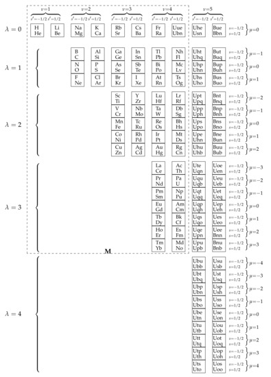
Figure 2. Seaborg table in the form of the basic representation $F_{s{s}^{\prime }}^{+}$ of the Rumer–Fet group (basis $|\nu ,\lambda ,\mu ,s,s^{\prime }⟩$). The dashed frame indicates the Mendeleev table.

Let us calculate the average masses of these multiplets. With this aim in view, we use mass formula (10). Formula (10) corresponds to the chain of groups (9), according to which we have a reduction of the basic representation $F_{s{s}^{\prime }}^{+}$ on the subgroups of this chain; that is, a partition of the basic multiplets into the lesser multiplets. As noted above, Formula (10) is analogous to the “first perturbation” in $\mathrm{SU}\left(3\right)$ and $\mathrm{SU}\left(6\right)$-theories, which allows us to calculate an average mass of the elements belonging to a given multiplet (therefore, in $\mathrm{SU}\left(3\right)$-theory we have a Gell-Mann–Okubo mass formula

$$m=m_0+\alpha +\beta Y+\gamma \left[I(I+1)-\frac{1}{4}{Y}^2\right]+{\alpha }^{\prime }-{\beta }^{\prime }Q+{\gamma }^{\prime }\left[U(U+1)-\frac{1}{4}{Q}^2\right],$$

in which, according to $\mathrm{SU}\left(3\right)/\mathrm{SU}\left(2\right)$-reduction, quantum numbers (isospin I, hypercharge Y), standing in the first square bracket, define the “first perturbation” that leads to a so-called hypercharge mass splitting; that is, a partition of the multiplet of $\mathrm{SU}\left(3\right)$ into the lesser multiplets of the subgroup $\mathrm{SU}\left(2\right)$. A “second perturbation” is defined by the quantum numbers, standing in the second square bracket (charge Q and isospin U, which, differently from I, corresponds to other choices of the basis in the subgroup $\mathrm{SU}\left(2\right)$), which leads to a charge mass splitting inside the multiplets of $\mathrm{SU}\left(2\right)$). At $m_0=1$, $a=17$, $b=5.5$ from (10) we obtain the average masses of multiplets (see Table 2).

Table 2. Average masses of multiplets of the Seaborg table.

	Multiplet	Mass (theor.)
1.	$(\nu =5,s^{\prime }=-1/2,\lambda =4)$	316
2.	$(\nu =5,s^{\prime }=-1/2,\lambda =3)$	360
3.	$(\nu =5,s^{\prime }=-1/2,\lambda =2)$	393
4.	$(\nu =5,s^{\prime }=-1/2,\lambda =1)$	415
5.	$(\nu =5,s^{\prime }=-1/2,\lambda =0)$	426
6.	$(\nu =5,s^{\prime }=1/2,\lambda =4)$	435
7.	$(\nu =5,s^{\prime }=1/2,\lambda =3)$	479
8.	$(\nu =5,s^{\prime }=1/2,\lambda =2)$	512
9.	$(\nu =5,s^{\prime }=1/2,\lambda =1)$	534
10.	$(\nu =5,s^{\prime }=1/2,\lambda =0)$	545

With the aim of obtaining an analog of the “second perturbation”, which leads to a mass splitting inside the multiplets of group $G_2=\mathrm{SO}\left(3\right)\otimes \mathrm{SU}\left(2\right)$, it needs to find a subsequent lengthening of the group chain $G\supset G_1\supset G_2$ (9). Therefore, we need to find another subgroup $G_3$. Then $G_2/G_3$-reduction gives a termwise mass splitting. As is known, a representation $\left\{u_O\right\}$ of group $\mathrm{SU}\left(2\right)$ compares each rotation O from $\mathrm{SO}\left(3\right)$ with the matrix $u_O$ from $\mathrm{SU}\left(2\right)$, and thereby the pair $(O,u_O)$; that is, the element of $G_2$. At the multiplication, $(O,u_O)$ give the pairs of the same form: $(O_1,u_{O_1})(O_2,u_{O_2})=(O_1{O}_2,u_{O_1}{u}_{O_2})=(O_1{O}_2,u_{O_1{O}_2})$, the reverse pairs are analogous: ${(O,u_O)}^{-1}=(O^{-1},u_{O^{-1}})$. Therefore, such pairs form subgroup $G_3$ in $G_2$. The subgroup $G_3$ is locally isomorphic to $\mathrm{SO}\left(3\right)$. Following Fet, we will denote it via $\mathrm{SO}{\left(3\right)}_c$. Further, one-parameter subgroups of group $\mathrm{SO}\left(3\right)$ have the form $\left\{e^{-i\alpha A_k}\right\}$ ($k=1,2,3$); since the representation $\left\{u_O\right\}$ converts them into one-parameter subgroups $\left\{e^{-i\alpha {\tau }_k}\right\}$ of group $\mathrm{SU}\left(2\right)$; then the corresponding one-parameter subgroups in $\mathrm{SO}{\left(3\right)}_c$ have the form

$$\left(e^{-i\alpha A_k},e^{-i\alpha {\tau }_k}\right)=\left(e^{-i\alpha A_k},1\right)\left(1,e^{-i\alpha {\tau }_k}\right).$$

Since the matrices $A_1$, $A_2$, $A_3$ correspond to the rotations ${\mathbf{L}}_{23}={\mathbf{J}}_1+{\mathbf{K}}_1$, ${\mathbf{L}}_{31}={\mathbf{J}}_2+{\mathbf{K}}_2$, ${\mathbf{L}}_{12}={\mathbf{J}}_3+{\mathbf{K}}_3$ in group G (in the basic representation of group G, see Section 2), the pair $\left(e^{-i\alpha A_k},1\right)$ is represented by the operator $e^{-i\alpha ({\mathbf{J}}_k+{\mathbf{K}}_k)}$, and the pair $\left(1,e^{-i\alpha {\tau }_k}\right)$ is represented by $e^{-i\alpha {\tau }_k}$. Thus, one-parameter subgroups of $G_3=\mathrm{SO}{\left(3\right)}_c$ correspond to subgroups of operators $e^{-i\alpha ({\mathbf{J}}_k+{\mathbf{K}}_k)}{e}^{-i\alpha {\tau }_k}$ ($k=1,2,3$). Irreducible representations of group $G_2=\mathrm{SO}\left(3\right)\otimes \mathrm{SU}\left(2\right)$ are numbered by the collections of quantum numbers $(\nu ,s^{\prime },\lambda )$. These representations form vertical rectangles in Figure 2. Each of them is defined by a fundamental representation of $\mathrm{SU}\left(2\right)$ and $(2\lambda +1)$-dimensional irreducible representation of group $\mathrm{SO}\left(3\right)$. At $G_2/G_3$-reduction from such a representation, we obtain an irreducible representation of the subgroup $G_3=\mathrm{SO}{\left(3\right)}_c$, for which a Clebsch–Gordan sequence $\left|j_1-j_2\right|$, …, $j_1+j_2$ with the values $j_1=1/2$ and $j_2=\lambda$ is reduced to two terms $\lambda -1/2$, $\lambda +1/2$ at $\lambda >0$ and to one term $1/2$ at $\lambda =0$. Therefore, at $\lambda >0$, the representation $(\nu ,s^{\prime },\lambda )$ of group $G_2$ is reduced to two irreducible representations of subgroup $G_3$ with dimensionality $2(\lambda -1/2)+1=2\lambda$ and $2(\lambda +1/2)+1=2\lambda +2$, and at $\lambda =0$ to one two-dimensional irreducible representation. Thus, at $\lambda >0$, multiplets of subgroup $G_2$ are reduced to two multiplets of subgroup $G_3$. $G_2/G_3$-reduction leads to the following (lengthened) chain of groups:

$$\begin{array}{c}G\supset G_1\supset G_2\supset G_3⟼\hfill \\ \hfill \mathrm{SO}(2,4)\otimes \mathrm{SU}\left(2\right)\otimes \mathrm{SU}\left(2\right)\supset \mathrm{SO}\left(4\right)\otimes \mathrm{SU}\left(2\right)\supset \mathrm{SO}\left(3\right)\otimes \mathrm{SU}\left(2\right)\supset \mathrm{SO}{\left(3\right)}_c.\end{array}$$

(13)

The lengthening of the group chain requires the introduction of a new basis whose vectors belong to the smallest multiplets of symmetry; that is, multiplets of the subgroup $G_3$. The vectors $|\nu ,\lambda ,\mu ,s,s^{\prime }⟩$ of basis (8), corresponding to group chain (9), do not already compose a chosen (well-defined) basis, since $\mu$, s do not belong to quantum numbers of the symmetry group; that is, these vectors do not belong to irreducible spaces of group $G_3$. The new basis is defined as follows. Since $\nu$, $s^{\prime }$, $\lambda$ are related to the groups G, $G_1$, $G_2$, they remain quantum numbers of chain (9), and instead, $\mu$, s have new quantum numbers related to $G_3$. First, quantum number ${\iota }_{\lambda }$ relates with the Casimir operator of the subgroup $G_3$, which is equal to ${\sum }_{k=1}^3{({\mathit{\tau }}_k+{\mathbf{J}}_k+{\mathbf{K}}_k)}^2$. At this point, two multiplets of $G_3$, obtained at the $G_2/G_3$-reduction, correspond to ${\iota }_{\lambda }=\lambda -1/2$ and ${\iota }_{\lambda }=\lambda +1/2$, whence $2\lambda =2{\iota }_{\lambda }+1$, $2\lambda +2=2{\iota }_{\lambda }+1$. Another quantum number, $\kappa$, is an eigenvalue of the operator $q_3={\mathit{\tau }}_3+{\mathbf{J}}_3+{\mathbf{K}}_3$, which belongs to the Lie algebra of group $G_3=\mathrm{SO}{\left(3\right)}_c$. Thus, the new basis, corresponding to the group chain (13), has the form

$$\begin{array}{c}|\nu ,s^{\prime },\lambda ,{\iota }_{\lambda },\kappa ⟩,\nu =1,2,\dots ;s^{\prime }=-1/2,1/2\lambda =0,1,\dots ,\nu -1;\hfill \\ \hfill {\iota }_{\lambda }=\lambda -1/2,\lambda +1/2\kappa =-{\iota }_{\lambda },-{\iota }_{\lambda }+1,\dots ,{\iota }_{\lambda }-1,{\iota }_{\lambda }.\end{array}$$

(14)

The Seaborg table recorded in basis (14), is shown in Figure 3.

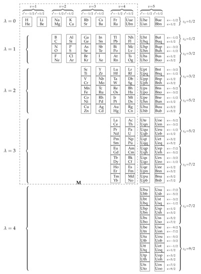
Figure 3. The Seaborg table in the form of the basic representation $F_{s{s}^{\prime }}^{+}$ of the Rumer–Fet group (basis $|\nu ,s^{\prime },\lambda ,{\iota }_{\lambda },\kappa ⟩$).

Masses of Elements

The lengthened group chain $G\supset G_1\supset G_2\supset G_3$ (13) allows us to provide a termwise mass splitting of the basic representation $F_{s{s}^{\prime }}^{+}$ of the Rumer–Fet group. With this aim in view, we introduce the following mass formula:

$$\begin{array}{c}m=m_0+a\left[s^{\prime }(2\nu -3)-5\nu +\frac{11}{2}+2({\nu }^2-1)\right]-b·\lambda (\lambda +1)+\hfill \\ \hfill +a^{\prime }\left[2\kappa -0,1666{\kappa }^3+0,0083{\kappa }^5-0,0001{\kappa }^7\right]+{\left(b^{\prime }{\iota }_{\lambda }\right)}^p-1,\end{array}$$

(15)

where

$$p=\left\{\begin{array}{cc}\hfill 0,& \mathrm{if}{\iota }_{\lambda }=\lambda -1/2;\hfill \\ \hfill 1,& \mathrm{if}{\iota }_{\lambda }=\lambda +1/2.\hfill \end{array}\right.$$

As the “first perturbation”, we have in (15), the Fet formula (10), corresponding to the group chain (9), where the basic representation $F_{s{s}^{\prime }}^{+}$ is divided into the multiplets $(\nu ,s^{\prime },\lambda )$ with average masses of $(\nu ,s^{\prime },\lambda )$. An analog of the “second perturbation” in formula (15) is defined by quantum numbers ${\iota }_{\lambda }$, $\kappa$, which, according to chain (13), leads to a partition of the multiplets $(\nu ,s^{\prime },\lambda )$ into the pair of multiplets of subgroup $G_3$ ($G_2/G_3$-reduction), and thereby we have here a termwise mass splitting.

We now calculate the masses of the elements of the Seaborg table, including the masses of the elements of the Mendeleev table, since the latter is part of the Seaborg table. For this purpose, in addition to the average weights of heavy multiplets (see Table 1), we calculate the average masses of the light multiplets of the Mendeleev table using the Fet formula (10) for the values $m_0=8,0$, $a=16,1$, $b=5.0$. The results are shown in Table 3.

Table 3. Average masses of the light multiplets of the Mendeleev table.

	Multiplet	Mass (exp.)	Mass (theor.)	Approx. %
1.	$(\nu =1,s^{\prime }=-1/2,\lambda =0)$	$2.505$
2.	$(\nu =1,s^{\prime }=1/2,\lambda =0)$	$7.975$	8.00	+0.31
3.	$(\nu =2,s^{\prime }=-1/2,\lambda =1)$	$15.335$	14.10	−8.05
4.	$(\nu =2,s^{\prime }=-1/2,\lambda =0)$	$23.65$	24.10	+1.90
5.	$(\nu =2,s^{\prime }=1/2,\lambda =1)$	$32.25$	30.20	−6.35
6.	$(\nu =2,s^{\prime }=1/2,\lambda =0)$	$39.59$	40.20	+1.54

The accuracy of the description is comparable to that obtained for hadron multiplets, with the exception of the multiplet $(\nu =1,s^{\prime }=-1/2,\lambda =0)$ containing H and He.

The masses of the elements of the periodic system, starting from the atomic number $Z=3$ to $Z=20$, are calculated according to mass formula (15) at values $m_0=8.0$, $a=16.1$, $b=5.0$, $a^{\prime }=2.15$, $b^{\prime }=5.3$ (light multiplets of the Mendeleev table) and at $m_0=1$, $a=17$, $b=5.5$, $a^{\prime }=1.1$, $b^{\prime }=3.9$ for heavy multiplets, starting from $Z=21$ to $Z=120$ (see Table 4). The first column of Table 4 contains the atomic number of the element; in the second column, we have a generally accepted (according to IUPAC—International Union of Pure and Applied Chemistry) designation of the element; the third column contains the quantum numbers of the element defining the vector $|\nu ,s^{\prime },\lambda ,{\iota }_{\lambda },\kappa ⟩$ of the basis (14) (recall, that according to the group-theoretical description, each element of the periodic system corresponds to the vector $|\nu ,s^{\prime },\lambda ,{\iota }_{\lambda },\kappa ⟩$ of the basis (14), thereby forming a single quantum system); the fourth column shows the experimental mass of the element; the fifth column contains the theoretical mass of the element calculated using Formula (15); the sixth column contains the relative error between the experimental and the calculated values.

Table 4. The masses of elements of the Mendeleev table.

Z	Element	Vector $|\mathit{\nu },{\mathit{s}}^{\prime },\mathit{\lambda },{\mathit{\iota }}_{\mathit{\lambda }},\mathit{\kappa }⟩$	Mass (exp.)	Mass (theor.)	Approx. %
1	H	$|1,-1/2,0,1/2,-1/2⟩$	1.01
2	He	$|1,-1/2,0,1/2,1/2⟩$	4.00
3	Li	$|1,1/2,0,1/2,-1/2⟩$	6.94	$5.89$	$-15.19$
4	Be	$|1,1/2,0,1/2,1/2⟩$	9.01	$10.10$	$+12.09$
5	B	$|2,-1/2,1,1/2,-1/2⟩$	10.81	$11.89$	$+10.91$
6	C	$|2,-1/2,1,1/2,1/2⟩$	12.01	$16.20$	$+34.89$
7	N	$|2,-1/2,1,3/2,-3/2⟩$	14.01	$15.67$	$+11.85$
8	O	$|2,-1/2,1,3/2,-1/2⟩$	16.00	$18.94$	$+18.37$
9	F	$|2,-1/2,1,3/2,1/2⟩$	19.00	$23.15$	$+21.84$
10	Ne	$|2,-1/2,1,3/2,3/2⟩$	20.18	$26.42$	$+30.92$
11	Na	$|2,-1/2,0,1/2,-1/2⟩$	22.99	$21.99$	$-4.35$
12	Mg	$|2,-1/2,0,1/2,1/2⟩$	24.31	$26.20$	$+7.77$
13	Al	$|2,1/2,1,1/2,-1/2⟩$	26.98	$28.09$	$+4.11$
14	Si	$|2,1/2,1,1/2,1/2⟩$	28.09	32.30	+14.38
15	P	$|2,1/2,1,3/2,-3/2⟩$	30.97	31.77	+2.58
16	S	$|2,1/2,1,3/2,-1/2⟩$	32.06	35.04	+9.29
17	Cl	$|2,1/2,1,3/2,1/2⟩$	35.45	39.25	+10.72
18	Ar	$|2,1/2,1,3/2,-3/2⟩$	39.95	42.52	+6.43
19	K	$|2,1/2,0,1/2,-1/2⟩$	39.10	38.09	−2.58
20	Ca	$|2,1/2,0,1/2,1/2⟩$	40.08	42.30	+5.54
21	Sc	$|3,-1/2,2,3/2,-3/2⟩$	44.96	50.25	+11.76
22	Ti	$|3,-1/2,2,3/2,-1/2⟩$	47.90	51.92	+8.39
23	V	$|3,-1/2,2,3/2,1/2⟩$	50.94	54.08	+6.16
24	Cr	$|3,-1/2,2,3/2,3/2⟩$	52.00	55.75	+7.21
25	Mn	$|3,-1/2,2,5/2,-5/2⟩$	54.94	58.28	+6.08
26	Fe	$|3,-1/2,2,5/2,-3/2⟩$	55.85	59.00	+5.64
27	Co	$|3,-1/2,2,5/2,-1/2⟩$	58.93	60.67	+2.95
28	Ni	$|3,-1/2,2,5/2,1/2⟩$	58.70	62.83	+7.03
29	Cu	$|3,-1/2,2,5/2,3/2⟩$	63.55	64.49	+1.48
30	Zn	$|3,-1/2,2,5/2,5/2⟩$	65.38	65.21	−0.26
31	Ga	$|3,-1/2,1,1/2,-1/2⟩$	69.72	73.92	+6.02
32	Ge	$|3,-1/2,1,1/2,1/2⟩$	72.59	76.08	+4.81
33	As	$|3,-1/2,1,3/2,-3/2⟩$	74.92	77.10	+2.91
34	Se	$|3,-1/2,1,3/2,-1/2⟩$	78.96	78.77	−0.24
35	Br	$|3,-1/2,1,3/2,1/2⟩$	79.90	80.93	+1.29
36	Kr	$|3,-1/2,1,3/2,3/2⟩$	83.80	82.60	−1.43
37	Rb	$|3,-1/2,0,1/2,-1/2⟩$	85.47	84.92	−0.64
38	Sr	$|3,-1/2,0,1/2,1/2⟩$	87.62	87.07	−0.63
39	Y	$|3,1/2,2,3/2,-3/2⟩$	88.91	101.25	+13.88
40	Zr	$|3,1/2,2,3/2,-1/2⟩$	91.22	102.92	+12.83
41	Nb	$|3,1/2,2,3/2,1/2⟩$	92.91	105.07	+13.09
42	Mo	$|3,1/2,2,3/2,3/2⟩$	95.94	106.75	+11.27
43	Tc	$|3,1/2,2,5/2,-5/2⟩$	98.91	109.28	+10.48
44	Ru	$|3,1/2,2,5/2,-3/2⟩$	101.07	110.00	+8.83
45	Rh	$|3,1/2,2,5/2,-1/2⟩$	102.91	111.67	+8.51
46	Pd	$|3,1/2,2,5/2,1/2⟩$	106.42	113.83	+6.96
47	Ag	$|3,1/2,2,5/2,3/2⟩$	107.87	115.49	+7.06
48	Cd	$|3,1/2,2,5/2,5/2⟩$	112.41	116.21	+3.38
49	In	$|3,1/2,1,1/2,-1/2⟩$	114.82	124.92	+8.79
50	Sn	$|3,1/2,1,1/2,1/2⟩$	118.69	127.07	+7.06
51	Sb	$|3,1/2,1,3/2,-3/2⟩$	121.75	128.10	+5.21
52	Te	$|3,1/2,1,3/2,-1/2⟩$	127.60	129.77	+1.77
53	I	$|3,1/2,1,3/2,1/2⟩$	126.90	131.02	+3.96
54	Xe	$|3,1/2,1,3/2,3/2⟩$	131.30	133.59	+1.74
55	Cs	$|3,1/2,0,1/2,-1/2⟩$	132.91	135.92	+2.26
56	Ba	$|3,1/2,0,1/2,1/2⟩$	137.33	138.08	+0.55
57	La	$|4,-1/2,3,5/2,-5/2⟩$	138.91	152.53	+9.80
58	Ce	$|4,-1/2,3,5/2,-3/2⟩$	140.12	153.25	+9.37
59	Pr	$|4,-1/2,3,5/2,-1/2⟩$	140.91	154.92	+9.94
60	Nd	$|4,-1/2,3,5/2,1/2⟩$	144.24	157.07	+8.89
61	Pm	$|4,-1/2,3,5/2,3/2⟩$	[145]	158.75	+9.48
62	Sm	$|4,-1/2,3,5/2,5/2⟩$	150.40	159.46	+6.02
63	Eu	$|4,-1/2,3,7/2,-7/2⟩$	151.96	164.72	+8.39
64	Gd	$|4,-1/2,3,7/2,-5/2⟩$	157.25	165.18	+5.04
65	Tb	$|4,-1/2,3,7/2,-3/2⟩$	158.93	165.90	+4.38
66	Dy	$|4,-1/2,3,7/2,-1/2⟩$	162.50	167.52	+3.09
67	Ho	$|4,-1/2,3,7/2,1/2⟩$	164.93	169.72	+2.90
68	Er	$|4,-1/2,3,7/2,3/2⟩$	167.26	171.39	+2.47
69	Tm	$|4,-1/2,3,7/2,5/2⟩$	168.93	172.11	+1.88
70	Eu	$|4,-1/2,3,7/2,7/2⟩$	173.04	172.58	−0.26
71	Lu	$|4,-1/2,2,3/2,-3/2⟩$	174.97	186.25	+6.45
72	Hf	$|4,-1/2,2,3/2,-1/2⟩$	178.49	187.92	+5.28
73	Ta	$|4,-1/2,2,3/2,1/2⟩$	180.95	190.07	+5.04
74	W	$|4,-1/2,2,3/2,3/2⟩$	183.85	191.75	+4.29
75	Re	$|4,-1/2,2,5/2,-5/2⟩$	186.21	194.28	+4.33
76	Os	$|4,-1/2,2,5/2,-3/2⟩$	190.20	195.00	+2.52
77	Ir	$|4,-1/2,2,5/2,-1/2⟩$	192.22	196.67	+2.31
78	Pt	$|4,-1/2,2,5/2,1/2⟩$	195.09	198.82	+1.91
79	Au	$|4,-1/2,2,5/2,3/2⟩$	196.97	200.49	+1.79
80	Hg	$|4,-1/2,2,5/2,5/2⟩$	200.59	201.21	+0.30
81	Tl	$|4,-1/2,1,1/2,-1/2⟩$	204.37	209.92	+2.71
82	Pb	$|4,-1/2,1,1/2,1/2⟩$	207.20	212.07	+2.35
83	Bi	$|4,-1/2,1,3/2,-3/2⟩$	208.98	213.10	+1.97
84	Po	$|4,-1/2,1,3/2,-1/2⟩$	208.98	214.77	+2.77
85	At	$|4,-1/2,1,3/2,1/2⟩$	[210]	216.93	+3.30
86	Rn	$|4,-1/2,1,3/2,3/2⟩$	222.08	218.60	−1.57
87	Fr	$|4,-1/2,0,1/2,-1/2⟩$	223.08	220.92	−0.97
88	Ra	$|4,-1/2,0,1/2,1/2⟩$	226.03	223.07	−1.31
89	Ac	$|4,1/2,3,5/2,-5/2⟩$	227.03	237.53	+4.62
90	Th	$|4,1/2,3,5/2,-3/2⟩$	232.04	238.25	+2.67
91	Pa	$|4,1/2,3,5/2,-1/2⟩$	231.04	239.92	+3.84
92	U	$|4,1/2,3,5/2,1/2⟩$	238.03	242.07	+1.69
93	Np	$|4,1/2,3,5/2,3/2⟩$	237.05	243.75	+2.82
94	Pu	$|4,1/2,3,5/2,5/2⟩$	244.06	244.46	+0.16
95	Am	$|4,1/2,3,7/2,-7/2⟩$	[243]	249.72	+2.76
96	Cm	$|4,1/2,3,7/2,-5/2⟩$	247.07	250.19	+1.26
97	Bk	$|4,1/2,3,7/2,-3/2⟩$	247.07	250.90	+1.55
98	Cf	$|4,1/2,3,7/2,-1/2⟩$	251.08	252.57	+0.59
99	Es	$|4,1/2,3,7/2,1/2⟩$	252.08	254.72	+1.08
100	Fm	$|4,1/2,3,7/2,3/2⟩$	257.09	256.40	−0.27
101	Md	$|4,1/2,3,7/2,5/2⟩$	258.10	257.11	−0.38
102	No	$|4,1/2,3,7/2,7/2⟩$	259.10	257.58	−0.59
103	Lr	$|4,1/2,2,3/2,-3/2⟩$	[266]	271.25	+1.93
104	Rf	$|4,1/2,2,3/2,-1/2⟩$	267	272.92	+2.22
105	Db	$|4,1/2,2,3/2,1/2⟩$	268	275.07	+2.64
106	Sg	$|4,1/2,2,3/2,3/2⟩$	[269]	276.75	+2.88
107	Bh	$|4,1/2,2,5/2,-5/2⟩$	[267]	279.28	+4.60
108	Hs	$|4,1/2,2,5/2,-3/2⟩$	[269]	280.00	+4.09
109	Mt	$|4,1/2,2,5/2,-1/2⟩$	[278]	281.67	+1.32
110	Ds	$|4,1/2,2,5/2,1/2⟩$	[281]	283.83	+1.01
111	Rg	$|4,1/2,2,5/2,3/2⟩$	[282]	285.50	+1.24
112	Cn	$|4,1/2,2,5/2,5/2⟩$	[285]	286.21	+0.42
113	Nh	$|4,1/2,1,1/2,-1/2⟩$	[286]	294.92	+3.12
114	Fl	$|4,1/2,1,1/2,1/2⟩$	[289]	297.08	+2.79
115	Mc	$|4,1/2,1,3/2,-3/2⟩$	[290]	298.10	+2.79
116	Lv	$|4,1/2,1,3/2,-1/2⟩$	[293]	299.77	+2.31
117	Ts	$|4,1/2,1,3/2,1/2⟩$	[294]	301.92	+2.69
118	Og	$|4,1/2,1,3/2,3/2⟩$	[294]	303.59	+3.26
119	Uue	$|4,1/2,0,1/2,-1/2⟩$		305.92
120	Ubn	$|4,1/2,0,1/2,1/2⟩$		308.08

It follows from Table 4 that the masses of the elements are described by Formula (15), meaning it is better the heavier the element; therefore, this formula can be considered as asymptotic.

Further, the masses of the elements of the Seaborg table, starting from the atomic number $Z=121$ to $Z=220$, are given in Table 5. As noted above, the Seaborg table is an extension of the Mendeleev table, highlighted in Figure 3 by a dotted border. Table 5 shows the masses of the elements outside the dotted frame. Unlike Table 4, in which all elements (with the exception of Uue and Ubn) are actually observable objects (atoms) with experimentally established mass values, all elements of Table 5 are hypothetical, the theoretical masses of which are calculated according to mass formula (15) at the values $m_0=1$, $a=17$, $b=5.5$, $a^{\prime }=2.15$, $b^{\prime }=5.3$ (see Table 5).

Table 5. Masses of elements of the Seaborg table.

Z	Element	Vector $|\mathit{\nu },{\mathit{s}}^{\prime },\mathit{\lambda },{\mathit{\iota }}_{\mathit{\lambda }},\mathit{\kappa }⟩$	Mass (theor.)
121	Ubu	$|5,-1/2,4,7/2,-7/2⟩$	312.07
122	Ubb	$|5,-1/2,4,7/2,-5/2⟩$	312.59
123	Ubt	$|5,-1/2,4,7/2,-3/2⟩$	313.25
124	Ubq	$|5,-1/2,4,7/2,-1/2⟩$	314.92
125	Ubp	$|5,-1/2,4,7/2,1/2⟩$	317.07
126	Ubn	$|5,-1/2,4,7/2,3/2⟩$	318.75
127	Ubs	$|5,-1/2,4,7/2,5/2⟩$	319.46
128	Ubo	$|5,-1/2,4,7/2,7/2⟩$	319.93
129	Ube	$|5,-1/2,4,9/2,-9/2⟩$	326.61
130	Utn	$|5,-1/2,4,9/2,-7/2⟩$	328.62
131	Utu	$|5,-1/2,4,9/2,-5/2⟩$	329.08
132	Utb	$|5,-1/2,4,9/2,-3/2⟩$	329.80
133	Utt	$|5,-1/2,4,9/2,-1/2⟩$	331.47
134	Utq	$|5,-1/2,4,9/2,1/2⟩$	333.63
135	Utp	$|5,-1/2,4,9/2,3/2⟩$	335.29
136	Uth	$|5,-1/2,4,9/2,5/2⟩$	336.01
137	Uts	$|5,-1/2,4,9/2,7/2⟩$	336.48
138	Uto	$|5,-1/2,4,9/2,9/2⟩$	338.49
139	Ute	$|5,-1/2,3,5/2,-5/2⟩$	356.54
140	Uqn	$|5,-1/2,3,5/2,-3/2⟩$	357.25
141	Uqu	$|5,-1/2,3,5/2,-1/2⟩$	358.92
142	Uqb	$|5,-1/2,3,5/2,1/2⟩$	361.07
143	Uqt	$|5,-1/2,3,5/2,3/2⟩$	362.75
144	Uqq	$|5,-1/2,3,5/2,5/2⟩$	363.46
145	Uqp	$|5,-1/2,3,7/2,-7/2⟩$	368.72
146	Uqh	$|5,-1/2,3,7/2,-5/2⟩$	369.19
147	Uqs	$|5,-1/2,3,7/2,-3/2⟩$	369.90
148	Uqo	$|5,-1/2,3,7/2,-1/2⟩$	371.57
149	Uqe	$|5,-1/2,3,7/2,1/2⟩$	373.72
150	Upn	$|5,-1/2,3,7/2,3/2⟩$	375.39
151	Upu	$|5,-1/2,3,7/2,5/2⟩$	376.11
152	Uqb	$|5,-1/2,3,7/2,7/2⟩$	376.58
153	Upt	$|5,-1/2,2,3/2,-3/2⟩$	390.25
154	Upq	$|5,-1/2,2,3/2,-1/2⟩$	391.92
155	Upp	$|5,-1/2,2,3/2,1/2⟩$	394.08
156	Uph	$|5,-1/2,2,3/2,3/2⟩$	395.75
157	Ups	$|5,-1/2,2,5/2,-5/2⟩$	398.28
158	Upo	$|5,-1/2,2,5/2,-3/2⟩$	399.00
159	Upe	$|5,-1/2,2,5/2,-1/2⟩$	400.67
160	Uhn	$|5,-1/2,2,5/2,1/2⟩$	402.83
161	Uhu	$|5,-1/2,2,5/2,3/2⟩$	404.50
162	Uhb	$|5,-1/2,2,5/2,5/2⟩$	405.21
163	Uht	$|5,-1/2,1,1/2,-1/2⟩$	413.92
164	Uhq	$|5,-1/2,1,1/2,1/2⟩$	416.07
165	Uhp	$|5,-1/2,1,3/2,-3/2⟩$	417.10
166	Uhn	$|5,-1/2,1,3/2,-1/2⟩$	418.77
167	Uhs	$|5,-1/2,1,3/2,1/2⟩$	420.93
168	Uho	$|5,-1/2,1,3/2,3/2⟩$	422.59
169	Uhe	$|5,-1/2,0,1/2,-1/2⟩$	424.92
170	Usn	$|5,-1/2,0,1/2,1/2⟩$	427.08
171	Usu	$|5,1/2,4,7/2,-7/2⟩$	431.07
172	Usb	$|5,1/2,4,7/2,-5/2⟩$	431.54
173	Ust	$|5,1/2,4,7/2,-3/2⟩$	432.55
174	Usq	$|5,1/2,4,7/2,-1/2⟩$	433.92
175	Usp	$|5,1/2,4,7/2,1/2⟩$	436.08
176	Ush	$|5,1/2,4,7/2,3/2⟩$	437.75
177	Uss	$|5,1/2,4,7/2,5/2⟩$	438.46
178	Uso	$|5,1/2,4,7/2,7/2⟩$	438.93
179	Use	$|5,1/2,4,9/2,-9/2⟩$	445.61
180	Uon	$|5,1/2,4,9/2,-7/2⟩$	447.62
181	Uou	$|5,1/2,4,9/2,-5/2⟩$	448.09
182	Uob	$|5,1/2,4,9/2,-3/2⟩$	448.80
183	Uot	$|5,1/2,4,9/2,-1/2⟩$	450.47
184	Uoq	$|5,1/2,4,9/2,1/2⟩$	452.63
185	Uop	$|5,1/2,4,9/2,3/2⟩$	454.30
186	Uoh	$|5,1/2,4,9/2,5/2⟩$	455.01
187	Uos	$|5,1/2,4,9/2,7/2⟩$	455.48
188	Uoo	$|5,1/2,4,9/2,9/2⟩$	457.49
189	Uoe	$|5,1/2,3,5/2,-5/2⟩$	475.54
190	Uen	$|5,1/2,3,5/2,-3/2⟩$	476.25
191	Ueu	$|5,1/2,3,5/2,-1/2⟩$	477.92
192	Ueb	$|5,1/2,3,5/2,1/2⟩$	480.07
193	Uet	$|5,1/2,3,5/2,3/2⟩$	481.75
194	Ueq	$|5,1/2,3,5/2,5/2⟩$	482.46
195	Uep	$|5,1/2,3,7/2,-7/2⟩$	487.72
196	Ueh	$|5,1/2,3,7/2,-5/2⟩$	488.19
197	Ues	$|5,1/2,3,7/2,-3/2⟩$	488.90
198	Ueo	$|5,1/2,3,7/2,-1/2⟩$	490.57
199	Uee	$|5,1/2,3,7/2,1/2⟩$	492.73
200	Bnn	$|5,1/2,3,7/2,3/2⟩$	494.40
201	Bnu	$|5,1/2,3,7/2,5/2⟩$	495.11
202	Bnb	$|5,1/2,3,7/2,7/2⟩$	495.58
203	Bnt	$|5,1/2,2,3/2,-3/2⟩$	509.25
204	Bnq	$|5,1/2,2,3/2,-1/2⟩$	510.92
205	Bnp	$|5,1/2,2,3/2,1/2⟩$	513.08
206	Bnh	$|5,1/2,2,3/2,3/2⟩$	514.75
207	Bns	$|5,1/2,2,5/2,-5/2⟩$	517.29
208	Bno	$|5,1/2,2,5/2,-3/2⟩$	518.00
209	Bne	$|5,1/2,2,5/2,-1/2⟩$	519.67
210	Bun	$|5,1/2,2,5/2,1/2⟩$	521.83
211	Buu	$|5,1/2,2,5/2,3/2⟩$	523.50
212	Bub	$|5,1/2,2,5/2,5/2⟩$	524.21
213	But	$|5,1/2,1,1/2,-1/2⟩$	532.92
214	Buq	$|5,1/2,1,1/2,1/2⟩$	535.08
215	Bup	$|5,1/2,1,3/2,-3/2⟩$	536.10
216	Buh	$|5,1/2,1,3/2,-1/2⟩$	537.77
217	Bus	$|5,1/2,1,3/2,1/2⟩$	539.93
218	Buo	$|5,1/2,1,3/2,3/2⟩$	541.60
219	Bue	$|5,1/2,0,1/2,-1/2⟩$	543.92
220	Bbn	$|5,1/2,0,1/2,1/2⟩$	546.08

5. 10-Periodic Extension

The structure of the symmetry group of the periodic system, which is essentially a mathematical formulation of the Madelung rule (doubling periods), allows us to further expand the Mendeleev table, inclusive of 10th and 11th periods, etc. All elements of this extension are hypothetical. The main purpose of this section is to demonstrate that the 7 periods of the Mendeleev table are only the first steps of a broader mathematical structure.

Figure 4 shows a 10-periodic extension of the Mendeleev table in the form of the basic representation $F_{s{s}^{\prime }}^{+}$ of the Rumer–Fet group G for the basis (14). The Mendeleev and Seaborg tables are separated by dotted frames with the symbols M and S, respectively. The first period of the Mendeleev table, including hydrogen H and helium He, corresponds to the simplest multiplet $(\nu =1,s^{\prime }=-1/2,\lambda =0,{\iota }_{\lambda }=1/2)$ of group G. The second period consists of three multiplets: lithium Li and beryllium Be$(\nu =1,s^{\prime }=1/2,\lambda =0,{\iota }_{\lambda }=1/2)$, boron B and carbon C $(\nu =2,s^{\prime }=-1/2,\lambda =0,{\iota }_{\lambda }=1/2)$, elements N, O, F, Ne form a quadruplet $(\nu =2,s^{\prime }=-1/2,\lambda =1,{\iota }_{\lambda }=3/2)$. The third period consists of three multiplets also (two doublets and one quadruplet): doublet Na and Mg $(\nu =2,s^{\prime }=-1/2,\lambda =0,{\iota }_{\lambda }=1/2)$, doublet Al and Si $(\nu =2,s^{\prime }=1/2,\lambda =1,{\iota }_{\lambda }=1/2)$, quadruplet P, S, Cl, Ar $(\nu =2,s^{\prime }=1/2,\lambda =1,{\iota }_{\lambda }=3/2)$. The fourth period includes five multiplets: doublets K, Ca $(\nu =2,s^{\prime }=1/2,\lambda =0,{\iota }_{\lambda }=1/2)$ and Ga, Ge $(\nu =3,s^{\prime }=-1/2,\lambda =1,{\iota }_{\lambda }=1/2)$, quadruplets As, Se, Br, Kr $(\nu =3,s^{\prime }=-1/2,\lambda =1,{\iota }_{\lambda }=3/2)$ and Sc, Ti, V, Cr $(\nu =3,s^{\prime }=-1/2,\lambda =2,{\iota }_{\lambda }=3/2)$, and also a sextet $(\nu =3,s^{\prime }=-1/2,\lambda =2,{\iota }_{\lambda }=5/2)$ formed by the elements Mn, …, Zn. This sextet and quadruplet $(\nu =3,s^{\prime }=-1/2,\lambda =2,{\iota }_{\lambda }=3/2)$ form the first insertion decade (transitional elements). The fifth period has an analogous structure: doublets Rb, Sr $(\nu =3,s^{\prime }=-1/2,\lambda =0,{\iota }_{\lambda }=1/2)$ and In, Sn $(\nu =3,s^{\prime }=1/2,\lambda =1,{\iota }_{\lambda }=1/2)$, quadruplet Sb, Te, I, Xe $(\nu =3,s^{\prime }=1/2,\lambda =1,{\iota }_{\lambda }=3/2)$, quadruplet Y, Zr, Nb, Mo $(\nu =3,s^{\prime }=1/2,\lambda =2,{\iota }_{\lambda }=3/2)$ and sextet Tc, …, Cd $(\nu =3,s^{\prime }=1/2,\lambda =2,{\iota }_{\lambda }=5/2)$ (the second insertion decade). The sixth period consists of seven multiplets: doublets Cs,Ba $(\nu =3,s^{\prime }=1/2,\lambda =0,{\iota }_{\lambda }=1/2)$ and Tl, Pb $(\nu =4,s^{\prime }=-1/2,\lambda =1,{\iota }_{\lambda }=1/2)$, quadruplets Bi, Po, At, Rn $(\nu =4,s^{\prime }=-1/2,\lambda =1,{\iota }_{\lambda }=3/2)$ and Lu, Hf, Ta, W $(\nu =4,s^{\prime }=-1/2,\lambda =2,{\iota }_{\lambda }=3/2)$, sextets Re, …, Hg $(\nu =4,s^{\prime }=-1/2,\lambda =2,{\iota }_{\lambda }=5/2)$ and La, …, Sm $(\nu =4,s^{\prime }=-1/2,\lambda =3,{\iota }_{\lambda }=5/2)$, octet Eu, …, Yb $(\nu =4,s^{\prime }=-1/2,\lambda =3,{\iota }_{\lambda }=7/2)$.

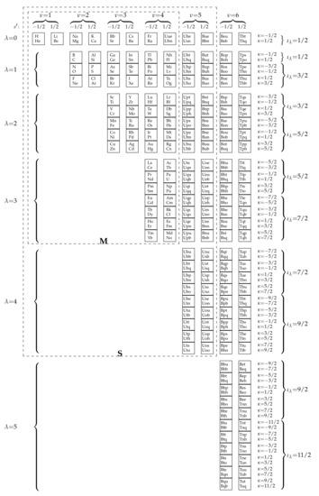
Figure 4. The 10-periodic extension of the Mendeleev table in the form of the basic representation $F_{s{s}^{\prime }}^{+}$ of the Rumer–Fet group (basis $|\nu ,s^{\prime },\lambda ,{\iota }_{\lambda },\kappa ⟩$). Dashed frames with the symbols M and S denote the Mendeleev and Seaborg tables, respectively.

The seventh period (the last period of the Mendeleev table) duplicates the structure of the sixth period: doublets Fr, Ra $(\nu =4,s^{\prime }=-1/2,\lambda =0,{\iota }_{\lambda }=1/2)$ and Nh, Fl $(\nu =4,s^{\prime }=1/2,\lambda =1,{\iota }_{\lambda }=1/2)$, quadruplets Mc, Lv, Ts, Og $(\nu =4,s^{\prime }=1/2,\lambda =1,{\iota }_{\lambda }=3/2)$ and Lr, Rf, Db, Sg $(\nu =4,s^{\prime }=1/2,\lambda =2,{\iota }_{\lambda }=3/2)$, sextets Bh, …, Cn $(\nu =4,s^{\prime }=1/2,\lambda =2,{\iota }_{\lambda }=5/2)$ and Ac, …, Pu $(\nu =4,s^{\prime }=1/2,\lambda =3,{\iota }_{\lambda }=5/2)$, octet Am, …, No $(\nu =4,s^{\prime }=1/2,\lambda =3,{\iota }_{\lambda }=7/2)$. The eighth period (the domain of hypothetical (undiscovered) elements of the periodic system begins with the eighth period), forming an 8-periodic extension of the Mendeleev table (Seaborg table), consists of nine multiplets: doublets Uue, Ubn $(\nu =4,s^{\prime }=1/2,\lambda =0,{\iota }_{\lambda }=1/2)$ and Uht, Uhq $(\nu =5,s^{\prime }=-1/2,\lambda =1,{\iota }_{\lambda }=1/2)$, quadruplets Uhp, …, Uho $(\nu =5,s^{\prime }=-1/2,\lambda =1,{\iota }_{\lambda }=3/2)$ and Upt, …, Uph $(\nu =5,s^{\prime }=-1/2,\lambda =2,{\iota }_{\lambda }=3/2)$, sextets Ups, …, Uhb $(\nu =5,s^{\prime }=-1/2,\lambda =2,{\iota }_{\lambda }=5/2)$ and Ute, …, Uqq $(\nu =5,s^{\prime }=-1/2,\lambda =3,{\iota }_{\lambda }=5/2)$, octets Uqp, …, Upb $(\nu =5,s^{\prime }=-1/2,\lambda =3,{\iota }_{\lambda }=7/2)$ and Ubu, …, Ubo $(\nu =5,s^{\prime }=-1/2,\lambda =4,{\iota }_{\lambda }=7/2)$, decuplet Ube, …, Uto $(\nu =5,s^{\prime }=-1/2,\lambda =4,{\iota }_{\lambda }=9/2)$. According to the Bohr model, filling of the g-shell is started with the element Ubu (Unbiunium). An analog of the g-shell in the Rumer–Fet model is a family of multiplets with quantum number $\lambda =4$ of group G. The eighth period contains 50 elements. The ninth period, finishing the Seaborg table, also contains nine multiplets: doublets Uhe, Usn $(\nu =5,s^{\prime }=-1/2,\lambda =0,{\iota }_{\lambda }=1/2)$ and But, Buq $(\nu =5,s^{\prime }=1/2,\lambda =1,{\iota }_{\lambda }=1/2)$, quadruplets Bup, …, Buo $(\nu =5,s^{\prime }=1/2,\lambda =1,{\iota }_{\lambda }=3/2)$ and Bnt, …, Bnh $(\nu =5,s^{\prime }=1/2,\lambda =2,{\iota }_{\lambda }=3/2)$, sextets Bns, …, Bub $(\nu =5,s^{\prime }=1/2,\lambda =2,{\iota }_{\lambda }=5/2)$ and Uoe, …, Ueq $(\nu =5,s^{\prime }=1/2,\lambda =3,{\iota }_{\lambda }=5/2)$, octets Uep, …, Bnb $(\nu =5,s^{\prime }=1/2,\lambda =3,{\iota }_{\lambda }=7/2)$ and Usu, …, Uso $(\nu =5,s^{\prime }=1/2,\lambda =4,{\iota }_{\lambda }=7/2)$, decuplet Use, …, Uoo $(\nu =5,s^{\prime }=1/2,\lambda =4,{\iota }_{\lambda }=9/2)$. The construction of a family of multiplets with the quantum number $\lambda =5$ of group G is started with the tenth period (in the Bohr’s model it corresponds to the formation of h-shell). The tenth period consists of 11 multiplets: doublets Bue, Bbn $(\nu =5,s^{\prime }=1/2,\lambda =0,{\iota }_{\lambda }=1/2)$ and Bop, Boh $(\nu =6,s^{\prime }=-1/2,\lambda =1,{\iota }_{\lambda }=1/2)$, quadruplets Bos, …, Ben $(\nu =6,s^{\prime }=-1/2,\lambda =1,{\iota }_{\lambda }=3/2)$ and Bsp, …, Bso $(\nu =6,s^{\prime }=-1/2,\lambda =2,{\iota }_{\lambda }=3/2)$, sextets Bse, …, Boq $(\nu =6,s^{\prime }=-1/2,\lambda =2,{\iota }_{\lambda }=5/2)$ and Bhu, …, Bhh $(\nu =6,s^{\prime }=-1/2,\lambda =3,{\iota }_{\lambda }=5/2)$, octets Bhs, …, Bsq $(\nu =6,s^{\prime }=-1/2,\lambda =3,{\iota }_{\lambda }=7/2)$ and Bqt, …, Bpn $(\nu =6,s^{\prime }=-1/2,\lambda =4,{\iota }_{\lambda }=7/2)$, decuplets Bpu, …, Bhn $(\nu =6,s^{\prime }=-1/2,\lambda =4,{\iota }_{\lambda }=9/2)$ and Bbu, …, Bth $(\nu =6,s^{\prime }=-1/2,\lambda =5,{\iota }_{\lambda }=9/2)$, 12-plet Btu, …, Bqb $(\nu =6,s^{\prime }=-1/2,\lambda =5,{\iota }_{\lambda }=11/2)$. The eleventh period has an analogous structure: doublets Beu, Beb $(\nu =6,s^{\prime }=-1/2,\lambda =0,{\iota }_{\lambda }=1/2)$ and Tps, Tpo $(\nu =6,s^{\prime }=1/2,\lambda =1,{\iota }_{\lambda }=1/2)$, quadruplets Tpe, …, Thb $(\nu =6,s^{\prime }=1/2,\lambda =1,{\iota }_{\lambda }=3/2)$ and Tqs, …, Tpn $(\nu =6,s^{\prime }=1/2,\lambda =2,{\iota }_{\lambda }=3/2)$, sextets Tpu, …, Tph $(\nu =6,s^{\prime }=1/2,\lambda =2,{\iota }_{\lambda }=5/2)$ and Ttt, …, Tto $(\nu =6,s^{\prime }=1/2,\lambda =3,{\iota }_{\lambda }=5/2)$, octets Tte, …, Tqh $(\nu =6,s^{\prime }=1/2,\lambda =3,{\iota }_{\lambda }=7/2)$ and Tup, …, Tbb $(\nu =6,s^{\prime }=1/2,\lambda =4,{\iota }_{\lambda }=7/2)$, decuplets Tbt, …, Ttb $(\nu =6,s^{\prime }=1/2,\lambda =4,{\iota }_{\lambda }=9/2)$ and Bet, …, Tnb $(\nu =6,s^{\prime }=1/2,\lambda =5,{\iota }_{\lambda }=9/2)$, 12-plet Tnt, …, Tuq $(\nu =6,s^{\prime }=1/2,\lambda =5,{\iota }_{\lambda }=11/2)$. The tenth and eleventh periods each contain 72 elements. The lengths of periods form the following number sequence:

$$2,8,8,18,18,32,32,50,50,72,72,\dots$$

(16)

The numbers of this sequence are defined by the famous Rydberg formula $2p^2$ (p is an integer number). The Rydberg series

$$R=2(1^2+1^2+2^2+2^2+3^2+3^2+4^2+4^2+\dots )$$

contains a doubled first period, which is somewhat inconsistent with reality; that is, sequence (16).

Further, the 12th period begins with the elements Tht (Trihexitrium, $Z=363$) and Thq (Trihexiquadium, $Z=364$), forming a doublet $(\nu =6,s^{\prime }=1/2,\lambda =0,{\iota }_{\lambda }=1/2)$. This period, already beyond the table in Figure 4, contains 13 multiplets. The length of the 12th period is equal to 98 (in exact correspondence with sequence (16)). A new family of multiplets with quantum number $\lambda =6$ of group G starts from the 12th period. This family corresponds to the i-shell filling. The 13th period has an analogous structure.

Obviously, as the quantum number $\nu$ increases, we will see new “steps” (doubled periods) and corresponding $\lambda$-families of multiplets (shells) in Figure 4.

Masses of Elements of 10th and 11th Periods

The table in Figure 4 corresponds to the reduction chain (13). Theoretical masses of elements of 10th and 11th periods, starting from $Z=221$ to $Z=364$, are calculated according to mass formula (15) at the values $m_0=1$, $a=17$, $b=5.5$, $a^{\prime }=2.15$, $b^{\prime }=5.3$ (see Table 6).

Table 6. Masses of elements of 10th and 11th periods.

Z	Element	Vector $|\mathit{\nu },{\mathit{s}}^{\prime },\mathit{\lambda },{\mathit{\iota }}_{\mathit{\lambda }},\mathit{\kappa }⟩$	Mass (theor.)
221	Bbu	$|6,-1/2,5,9/2,-9/2⟩$	527.06
222	Bbb	$|6,-1/2,5,9/2,-7/2⟩$	529.07
223	Bbt	$|6,-1/2,5,9/2,-5/2⟩$	529.54
224	Bbq	$|6,-1/2,5,9/2,-3/2⟩$	530.25
225	Bbp	$|6,-1/2,5,9/2,-1/2⟩$	531.92
226	Bbh	$|6,-1/2,5,9/2,1/2⟩$	534.08
227	Bbs	$|6,-1/2,5,9/2,3/2⟩$	535.75
228	Bbo	$|6,-1/2,5,9/2,5/2⟩$	536.46
229	Bbe	$|6,-1/2,5,9/2,7/2⟩$	536.93
230	Btn	$|6,-1/2,5,9/2,9/2⟩$	536.93
231	Btu	$|6,-1/2,5,11/2,-11/2⟩$	542.64
232	Btb	$|6,-1/2,5,11/2,-9/2⟩$	547.51
233	Btt	$|6,-1/2,5,11/2,-7/2⟩$	549.52
234	Btq	$|6,-1/2,5,11/2,-5/2⟩$	549.99
235	Btp	$|6,-1/2,5,11/2,-3/2⟩$	550.70
236	Bth	$|6,-1/2,5,11/2,-1/2⟩$	552.37
237	Bts	$|6,-1/2,5,11/2,1/2⟩$	554.53
238	Bto	$|6,-1/2,5,11/2,3/2⟩$	556.20
239	Bte	$|6,-1/2,5,11/2,5/2⟩$	556.91
240	Bqn	$|6,-1/2,5,11/2,7/2⟩$	557.38
241	Bqu	$|6,-1/2,5,11/2,9/2⟩$	559.39
242	Bqb	$|6,-1/2,5,11/2,11/2⟩$	564.26
243	Bqt	$|6,-1/2,4,7/2,-7/2⟩$	584.07
244	Bqq	$|6,-1/2,4,7/2,-5/2⟩$	584.54
245	Bqp	$|6,-1/2,4,7/2,-3/2⟩$	585.25
246	Bqh	$|6,-1/2,4,7/2,-1/2⟩$	586.92
247	Bqs	$|6,-1/2,4,7/2,1/2⟩$	589.08
248	Bqo	$|6,-1/2,4,7/2,3/2⟩$	590.75
249	Bqe	$|6,-1/2,4,7/2,5/2⟩$	591.46
250	Bpn	$|6,-1/2,4,7/2,7/2⟩$	591.93
251	Bpu	$|6,-1/2,4,9/2,-9/2⟩$	598.61
252	Bpb	$|6,-1/2,4,9/2,-7/2⟩$	600.62
253	Bpt	$|6,-1/2,4,9/2,-5/2⟩$	601.09
254	Bpq	$|6,-1/2,4,9/2,-3/2⟩$	601.80
255	Bpp	$|6,-1/2,4,9/2,-1/2⟩$	603.47
256	Bph	$|6,-1/2,4,9/2,1/2⟩$	605.63
257	Bps	$|6,-1/2,4,9/2,3/2⟩$	607.30
258	Bpo	$|6,-1/2,4,9/2,5/2⟩$	608.01
259	Bpe	$|6,-1/2,4,9/2,7/2⟩$	608.48
260	Bhn	$|6,-1/2,4,9/2,9/2⟩$	610.49
261	Bhu	$|6,-1/2,3,5/2,-5/2⟩$	628.54
262	Bhb	$|6,-1/2,3,5/2,-3/2⟩$	629.25
263	Bht	$|6,-1/2,3,5/2,-1/2⟩$	630.92
264	Bhq	$|6,-1/2,3,5/2,1/2⟩$	633.08
265	Bhp	$|6,-1/2,3,5/2,3/2⟩$	634.75
266	Bhh	$|6,-1/2,3,5/2,5/2⟩$	635.46
267	Bhs	$|6,-1/2,3,7/2,-7/2⟩$	640.72
268	Bho	$|6,-1/2,3,7/2,-5/2⟩$	641.19
269	Bhe	$|6,-1/2,3,7/2,-3/2⟩$	641.90
270	Bsn	$|6,-1/2,3,7/2,-1/2⟩$	643.57
271	Bsu	$|6,-1/2,3,7/2,1/2⟩$	645.73
272	Bsb	$|6,-1/2,3,7/2,3/2⟩$	647.40
273	Bst	$|6,-1/2,3,7/2,5/2⟩$	648.11
274	Bsq	$|6,-1/2,3,7/2,7/2⟩$	648.58
275	Bsp	$|6,-1/2,2,3/2,-3/2⟩$	662.25
276	Bsh	$|6,-1/2,2,3/2,-1/2⟩$	663.92
277	Bss	$|6,-1/2,2,3/2,1/2⟩$	666.08
278	Bso	$|6,-1/2,2,3/2,3/2⟩$	667.75
279	Bse	$|6,-1/2,2,5/2,-5/2⟩$	670.29
280	Bon	$|6,-1/2,2,5/2,-3/2⟩$	671.00
281	Bou	$|6,-1/2,2,5/2,-1/2⟩$	672.67
282	Bob	$|6,-1/2,2,5/2,1/2⟩$	674.83
283	Bot	$|6,-1/2,2,5/2,3/2⟩$	676.50
284	Boq	$|6,-1/2,2,5/2,5/2⟩$	677.21
285	Bop	$|6,-1/2,1,1/2,-1/2⟩$	685.92
286	Boh	$|6,-1/2,1,1/2,1/2⟩$	688.08
287	Bos	$|6,-1/2,1,3/2,-3/2⟩$	689.10
288	Boo	$|6,-1/2,1,3/2,-1/2⟩$	690.77
289	Boe	$|6,-1/2,1,3/2,1/2⟩$	692.93
290	Ben	$|6,-1/2,1,3/2,3/2⟩$	694.60
291	Beu	$|6,-1/2,0,1/2,-1/2⟩$	696.92
292	Beb	$|6,-1/2,0,1/2,1/2⟩$	699.08
293	Bet	$|6,1/2,5,9/2,-9/2⟩$	680.06
294	Beq	$|6,1/2,5,9/2,-7/2⟩$	682.07
295	Bep	$|6,1/2,5,9/2,-5/2⟩$	682.54
296	Beh	$|6,1/2,5,9/2,-3/2⟩$	683.25
297	Bes	$|6,1/2,5,9/2,-1/2⟩$	684.92
298	Beo	$|6,1/2,5,9/2,1/2⟩$	687.08
299	Bee	$|6,1/2,5,9/2,3/2⟩$	688.75
300	Tnn	$|6,1/2,5,9/2,5/2⟩$	689.46
301	Tnu	$|6,1/2,5,9/2,7/2⟩$	689.93
302	Tnb	$|6,1/2,5,9/2,9/2⟩$	691.94
303	Tnt	$|6,1/2,5,11/2,-11/2⟩$	695.64
304	Tnq	$|6,1/2,5,11/2,-9/2⟩$	700.51
305	Tnp	$|6,1/2,5,11/2,-7/2⟩$	702.52
306	Tnh	$|6,1/2,5,11/2,-5/2⟩$	702.59
307	Tns	$|6,1/2,5,11/2,-3/2⟩$	703.70
308	Tno	$|6,1/2,5,11/2,-1/2⟩$	705.37
309	Tne	$|6,1/2,5,11/2,1/2⟩$	707.53
310	Tun	$|6,1/2,5,11/2,3/2⟩$	709.20
311	Tuu	$|6,1/2,5,11/2,5/2⟩$	709.91
312	Tub	$|6,1/2,5,11/2,7/2⟩$	710.38
313	Tut	$|6,1/2,5,11/2,9/2⟩$	712.39
314	Tuq	$|6,1/2,5,11/2,11/2⟩$	717.26
315	Tup	$|6,1/2,4,7/2,-7/2⟩$	737.07
316	Tuh	$|6,1/2,4,7/2,-5/2⟩$	737.54
317	Tus	$|6,1/2,4,7/2,-3/2⟩$	738.25
318	Tuo	$|6,1/2,4,7/2,-1/2⟩$	739.92
319	Tue	$|6,1/2,4,7/2,1/2⟩$	742.08
320	Tbn	$|6,1/2,4,7/2,3/2⟩$	743.75
321	Tbu	$|6,1/2,4,7/2,5/2⟩$	744.46
322	Tbb	$|6,1/2,4,7/2,7/2⟩$	744.93
323	Tbt	$|6,1/2,4,9/2,-9/2⟩$	751.61
324	Tbq	$|6,1/2,4,9/2,-7/2⟩$	753.62
325	Tbp	$|6,1/2,4,9/2,-5/2⟩$	754.09
326	Tbh	$|6,1/2,4,9/2,-3/2⟩$	754.80
327	Tbs	$|6,1/2,4,9/2,-1/2⟩$	756.47
328	Tbo	$|6,1/2,4,9/2,1/2⟩$	758.63
329	Tbe	$|6,1/2,4,9/2,3/2⟩$	760.30
330	Ttn	$|6,1/2,4,9/2,5/2⟩$	761.01
331	Ttu	$|6,1/2,4,9/2,7/2⟩$	761.48
332	Ttb	$|6,1/2,4,9/2,9/2⟩$	763.49
333	Ttt	$|6,1/2,3,5/2,-5/2⟩$	781.54
334	Ttq	$|6,1/2,3,5/2,-3/2⟩$	782.25
335	Ttp	$|6,1/2,3,5/2,-1/2⟩$	783.92
336	Tth	$|6,1/2,3,5/2,1/2⟩$	786.08
337	Tts	$|6,1/2,3,5/2,3/2⟩$	787.75
338	Tto	$|6,1/2,3,5/2,5/2⟩$	788.46
339	Tte	$|6,1/2,3,7/2,-7/2⟩$	793.72
340	Tqn	$|6,1/2,3,7/2,-5/2⟩$	794.19
341	Tqu	$|6,1/2,3,7/2,-3/2⟩$	794.90
342	Tqb	$|6,1/2,3,7/2,-1/2⟩$	796.57
343	Tqt	$|6,1/2,3,7/2,1/2⟩$	798.73
344	Tqq	$|6,1/2,3,7/2,3/2⟩$	800.34
345	Tqp	$|6,1/2,3,7/2,5/2⟩$	801.11
346	Tqh	$|6,1/2,3,7/2,7/2⟩$	801.58
347	Tqs	$|6,1/2,2,3/2,-3/2⟩$	815.25
348	Tqo	$|6,1/2,2,3/2,-1/2⟩$	816.92
349	Tqe	$|6,1/2,2,3/2,1/2⟩$	819.08
350	Tpn	$|6,1/2,2,3/2,3/2⟩$	820.75
351	Tpu	$|6,1/2,2,5/2,-5/2⟩$	823.29
352	Tpb	$|6,1/2,2,5/2,-3/2⟩$	824.00
353	Tpt	$|6,1/2,2,5/2,-1/2⟩$	825.67
354	Tpq	$|6,1/2,2,5/2,1/2⟩$	827.83
355	Tpp	$|6,1/2,2,5/2,3/2⟩$	829.50
356	Tph	$|6,1/2,2,5/2,5/2⟩$	830.21
357	Tps	$|6,1/2,1,1/2,-1/2⟩$	838.92
358	Tpo	$|6,1/2,1,1/2,1/2⟩$	841.08
359	Tpe	$|6,1/2,1,3/2,-3/2⟩$	842.10
360	Thn	$|6,1/2,1,3/2,-1/2⟩$	843.77
361	Thu	$|6,1/2,1,3/2,1/2⟩$	845.93
362	Thb	$|6,1/2,1,3/2,3/2⟩$	847.60
363	Tht	$|6,1/2,0,1/2,-1/2⟩$	849.92
364	Thq	$|6,1/2,0,1/2,1/2⟩$	852.08

6. Homological Series

All elements of the extended table (see Figure 4), starting with hydrogen H ($Z=1$) and ending with Thq (Trihexiquadium, $Z=364$), form a single quantum system. Each element of the periodic system corresponds to the basis vector $|\nu ,s^{\prime },\lambda ,{\iota }_{\lambda },\kappa ⟩$, where $\nu$, $s^{\prime }$, $\lambda$, ${\iota }_{\lambda }$, $\kappa$ are quantum numbers of the symmetry group G (Rumer–Fet group). Thus, we have the following set of state vectors:

$$\begin{array}{ccc}\hfill |\mathbf{H}⟩\phantom{bn}& =& \left|1,-\frac{1}{2},0,\frac{1}{2},-\frac{1}{2}\right.⟩,\hfill \\ \hfill |\mathbf{He}⟩\phantom{n}& =& \left|1,-\frac{1}{2},0,\frac{1}{2},\frac{1}{2}\right.⟩,\hfill \\ \hfill |\mathbf{Li}⟩\phantom{bn}& =& \left|1,\frac{1}{2},0,\frac{1}{2},-\frac{1}{2}\right.⟩,\hfill \\ & & ⋮\hfill \\ \hfill |\mathbf{Thq}⟩& =& \left|6,\frac{1}{2},0,\frac{1}{2},\frac{1}{2}\right.⟩.\hfill \end{array}$$

(17)

In accordance with quantum mechanical laws, in aggregate (17), which forms a Hilbert space, we have linear superpositions of state vectors, as well as quantum transitions between different state vectors; that is, transitions between elements of the periodic system.

Let us now consider the operators that determine quantum transitions between the state vectors of the system (17):

$${\mathbf{\Gamma }}_{+}={\mathbf{P}}_{+}+{\mathbf{Q}}_{+},{\mathbf{\Gamma }}_{-}={\mathbf{P}}_{-}+{\mathbf{Q}}_{-}.$$

(18)

Operators (18) connect subspaces ${\mathfrak{F}}_n$ of the unitary representation $F^{+}$ of the conformal group $\mathrm{SO}(2,4)$ in the Fock space $\mathfrak{F}$. Indeed, the action of these operators on the basis vectors $|j,\sigma ,\tau ⟩$ of $\mathfrak{F}$ has the form

$$\begin{array}{c}{\mathbf{\Gamma }}_{+}|j,\sigma ,\tau ⟩=i\sqrt{(j+\sigma +1)(j-\tau +1)}\left|j+\frac{1}{2},\sigma +\frac{1}{2},\tau -\frac{1}{2}\right.⟩-\hfill \\ \hfill -i\sqrt{(j-\sigma +1)(j+\tau +1)}\left|j+\frac{1}{2},\sigma -\frac{1}{2},\tau +\frac{1}{2}\right.⟩,\end{array}$$

$$\begin{array}{c}{\mathbf{\Gamma }}_{-}|j,\sigma ,\tau ⟩=-i\sqrt{(j+\sigma )(j-\tau )}\left|j-\frac{1}{2},\sigma -\frac{1}{2},\tau +\frac{1}{2}\right.⟩+\hfill \\ \hfill +i\sqrt{(j-\sigma )(j+\tau )}\left|j-\frac{1}{2},\sigma +\frac{1}{2},\tau -\frac{1}{2}\right.⟩.\end{array}$$

Hence it follows that ${\mathbf{\Gamma }}_{+}$ transforms vectors of the subspace ${\mathfrak{F}}_n$ into vectors of ${\mathfrak{F}}_{n+1}$, since for the Fock representation ${\mathsf{\Phi }}_n=D_{\frac{n-1}{2},\frac{n-1}{2}}$ in the subspace ${\mathfrak{F}}_n$, where $j=\frac{n-1}{2}$, increasing the number j by $1/2$ means increasing the number n by 1 (see Appendix B). Analogously, the operator ${\mathbf{\Gamma }}_{-}$ transforms vectors of the subspace ${\mathfrak{F}}_n$ into vectors of ${\mathfrak{F}}_{n-1}$. Operators ${\mathbf{\Gamma }}_{+}$, ${\mathbf{\Gamma }}_{-}$ commute with the subgroup $G_2=\mathrm{SO}\left(3\right)\otimes \mathrm{SU}\left(2\right)$ belonging to the group chain (13). Indeed, in virtue of commutation relations of the conformal group $\mathrm{SO}(2,4)$ (see Section 2) it follows that

$$\left[{\mathbf{P}}_{\pm }+{\mathbf{Q}}_{\pm },{\mathbf{J}}_{+}+{\mathbf{K}}_{+}\right]=\left[{\mathbf{P}}_{\pm }+{\mathbf{Q}}_{\pm },{\mathbf{J}}_{-}+{\mathbf{K}}_{-}\right]=\left[{\mathbf{P}}_{\pm }+{\mathbf{Q}}_{\pm },{\mathbf{J}}_3+{\mathbf{K}}_3\right]=0.$$

Therefore, operators ${\mathbf{\Gamma }}_{+}$, ${\mathbf{\Gamma }}_{-}$ save quantum number $\mu$. Further, ${\mathbf{\Gamma }}_{+}$, ${\mathbf{\Gamma }}_{-}$ commute with a Casimir operator ${({\mathbf{J}}_1+{\mathbf{K}}_1)}^2+{({\mathbf{J}}_2+{\mathbf{K}}_2)}^2+{({\mathbf{J}}_3+{\mathbf{K}}_3)}^2$ of the subgroup $\mathrm{SO}\left(3\right)$, and thereby save quantum number $\lambda$. It is easy to see that ${\mathbf{\Gamma }}_{+}$, ${\mathbf{\Gamma }}_{-}$ commute with the operators ${\mathit{\tau }}_k$ ($k=1,2,3$) of the subgroup $\mathrm{SU}\left(2\right)$ and, therefore, they save quantum number s. Since ${\mathbf{\Gamma }}_{+}$ and ${\mathbf{\Gamma }}_{-}$ commute with ${\mathbf{J}}_k+{\mathbf{K}}_k$ and ${\mathit{\tau }}_k$ separately, then they commute with all of subgroup $G_2=\mathrm{SO}\left(3\right)\otimes \mathrm{SU}\left(2\right)$. Further, the operators ${\mathbf{\Gamma }}_{+}$, ${\mathbf{\Gamma }}_{-}$ commute with the subgroup $\mathrm{SU}{\left(2\right)}^{\prime }$, which defines the second “doubling”, and, therefore, they save quantum number $s^{\prime }$. Since ${\mathbf{\Gamma }}_{+}$ transforms ${\mathfrak{F}}_n$ into ${\mathfrak{F}}_{n+1}$, and ${\mathbf{\Gamma }}_{-}$ transforms ${\mathfrak{F}}_n$ into ${\mathfrak{F}}_{n-1}$, then in the space ${\mathfrak{F}}^4=C\left(2\right)\otimes {\mathfrak{F}}^2=C\left(2\right)\otimes [C\left(2\right)\otimes \mathfrak{F}]$ of the representation $F_{s{s}^{\prime }}^{+}$ the operator ${\mathbf{\Gamma }}_{+}$, ${\mathbf{\Gamma }}_{-}$ raises, and correspondingly, lowers quantum number $\nu$ by 1. Thus, for basis (8), the operator ${\mathbf{\Gamma }}_{+}$ saves quantum numbers $s^{\prime }$, $\lambda$, $\mu$, s, raising $\nu$ by the unit; therefore, ${\mathbf{\Gamma }}_{+}\left|\nu ,s^{\prime },\lambda ,\mu ,s\right.⟩=\eta |\nu +1,s^{\prime },\lambda ,\mu ,s⟩$, where $\eta \ne 0$. Analogously, ${\mathbf{\Gamma }}_{-}\left|\nu ,s^{\prime },\lambda ,\mu ,s\right.⟩={\eta }^{\prime }|\nu -1,s^{\prime },\lambda ,\mu ,s⟩$, where ${\eta }^{\prime }\ne 0$. Since ${\mathbf{\Gamma }}_{+}$ (correspondingly ${\mathbf{\Gamma }}_{-}$) defines an isomorphic mapping of the space of $(\nu ,s^{\prime },\lambda )$ onto the space of $(\nu +1,s^{\prime },\lambda )$ (corresp. $(\nu -1,s^{\prime },\lambda )$), then $\eta$ (corresp. ${\eta }^{\prime }$) does not depend on quantum numbers $\mu$, s. Therefore, for the vectors $|\nu ,s^{\prime },\lambda ,{\iota }_{\lambda },\kappa ⟩$ of the basis of (14) we have

$$\begin{array}{ccc}\hfill {\mathbf{\Gamma }}_{+}|\nu ,s^{\prime },\lambda ,{\iota }_{\lambda },\kappa ⟩& =& \eta |\nu +1,s^{\prime },\lambda ,{\iota }_{\lambda },\kappa ⟩,\hfill \end{array}$$

(19)

$$\begin{array}{ccc}\hfill {\mathbf{\Gamma }}_{-}|\nu ,s^{\prime },\lambda ,{\iota }_{\lambda },\kappa ⟩& =& {\eta }^{\prime }|\nu -1,s^{\prime },\lambda ,{\iota }_{\lambda },\kappa ⟩.\hfill \end{array}$$

(20)

Equality (20) holds at $0\le \lambda \le \nu -2$. A visual sense of the operators ${\mathbf{\Gamma }}_{+}$, ${\mathbf{\Gamma }}_{-}$ is that they move basic vectors, represented by cells in Figure 4, to the right, and correspondingly, to the left through horizontal columns of the table. At this point, ${\mathbf{\Gamma }}_{+}$ always transfers the basic vector of the column $(\nu ,s^{\prime })$ into the basic vector of the same parity $(\nu +1,s^{\prime })$ with multiplication by some non-null factor $\eta$. In turn, the operator ${\mathbf{\Gamma }}_{-}$ transfers the basis vector of the column $(\nu ,s^{\prime })$ into the basis vector of the same parity $(\nu -1,s^{\prime })$ with multiplication by a non-null factor ${\eta }^{\prime }$ when the column $(\nu -1,s^{\prime })$ contains a vector on the same horizontal, (otherwise we have zero).

Further, operators ${\mathit{\tau }}_{+}^{\prime }={\mathit{\tau }}_1^{\prime }+i{\mathit{\tau }}_2^{\prime }$, ${\mathit{\tau }}_{-}^{\prime }={\mathit{\tau }}_1^{\prime }-i{\mathit{\tau }}_2^{\prime }$ of the subgroup $\mathrm{SU}{\left(2\right)}^{\prime }$ also define quantum transitions between state vectors (17). Since these operators commute with the subgroup $G_1=\mathrm{SO}\left(4\right)\otimes \mathrm{SU}\left(2\right)$, they save quantum numbers $\nu$, $\lambda$, ${\iota }_{\lambda }$, $\kappa$, related with $G_1$, and change only quantum number $s^{\prime }$:

$$\begin{array}{ccc}\hfill {\mathbf{\tau }}_{+}^{\prime }\left|\nu ,-\frac{1}{2},\lambda ,{\iota }_{\lambda },\kappa \right.⟩& =& \left|\nu ,\frac{1}{2},\lambda ,{\iota }_{\lambda },\kappa \right.⟩,\hfill \end{array}$$

(21)

$$\begin{array}{ccc}\hfill {\mathit{\tau }}_{-}^{\prime }\left|\nu ,\frac{1}{2},\lambda ,{\iota }_{\lambda },\kappa \right.⟩\phantom{-}& =& \left|\nu ,-\frac{1}{2},\lambda ,{\iota }_{\lambda },\kappa \right.⟩.\hfill \end{array}$$

(22)

A visual sense of the operators ${\mathit{\tau }}_{+}^{\prime }$, ${\mathit{\tau }}_{-}^{\prime }$ is that ${\mathit{\tau }}_{+}^{\prime }$ moves basis vectors of each odd column (see Figure 4) horizontal into the basis vectors of the neighboring right column; in turn, ${\mathit{\tau }}_{-}^{\prime }$ moves the basis vectors of each even column horizontal into basis vectors of the neighboring left column. Thus, operators (19)–(22) define quantum transitions between state vectors of the system (17).

It is easy to see that on the horizontals of Figure 4 we have Mendeleev homological series; that is, families of elements with similar properties. Therefore, operators (19)–(22) define quantum transitions between elements of homological series. For example,

$$\begin{array}{c}{\mathbf{\Gamma }}_{+}|\mathbf{H}⟩={\mathbf{\Gamma }}_{+}\left|1,-\frac{1}{2},0,\frac{1}{2},-\frac{1}{2}\right.⟩={\eta }_1|\mathbf{Na}⟩={\eta }_1\left|2,-\frac{1}{2},0,\frac{1}{2},-\frac{1}{2}\right.⟩⟼\hfill \\ {\eta }_1{\mathbf{\Gamma }}_{+}|\mathbf{Na}⟩={\eta }_1{\eta }_2|\mathbf{Rb}⟩={\eta }_1{\eta }_2\left|3,-\frac{1}{2},0,\frac{1}{2},-\frac{1}{2}\right.⟩⟼\\ {\eta }_1{\eta }_2{\mathbf{\Gamma }}_{+}|\mathbf{Rb}⟩={\eta }_1{\eta }_2{\eta }_3|\mathbf{Fr}⟩={\eta }_1{\eta }_2{\eta }_3\left|4,-\frac{1}{2},0,\frac{1}{2},-\frac{1}{2}\right.⟩⟼\\ \hfill {\eta }_1{\eta }_2{\eta }_3{\mathbf{\Gamma }}_{+}|\mathbf{Fr}⟩={\eta }_1{\eta }_2{\eta }_3{\eta }_4|\mathbf{Uhe}⟩={\eta }_1{\eta }_2{\eta }_3{\eta }_4\left|5,-\frac{1}{2},0,\frac{1}{2},-\frac{1}{2}\right.⟩.\end{array}$$

Further, operators ${\mathit{\tau }}_{+}^{\prime }$, ${\mathit{\tau }}_{-}^{\prime }$ establish homology between lanthanides and actinides (this homology was first discovered by Seaborg. It is obvious that Seaborg homology is a particular case of the Mendeleev homology):

$${\mathit{\tau }}_{+}^{\prime }|\mathbf{La}⟩={\mathit{\tau }}_{+}^{\prime }\left|4,-\frac{1}{2},3,\frac{5}{2},-\frac{5}{2}\right.⟩=|\mathbf{Ac}⟩=\left|4,\frac{1}{2},3,\frac{5}{2},-\frac{5}{2}\right.⟩,$$

$$\begin{gathered} {\mathit{\tau }}_{+}^{\prime }|\mathbf{Ce}⟩={\tau }_{+}^{\prime }\left|4,-\frac{1}{2},3,\frac{5}{2},-\frac{3}{2}\right.⟩=|\mathbf{Th}⟩=\left|4,\frac{1}{2},3,\frac{5}{2},-\frac{3}{2}\right.⟩, \\ ⋮ \end{gathered}$$

$${\mathit{\tau }}_{+}^{\prime }|\mathbf{Yb}⟩={\mathit{\tau }}_{+}^{\prime }\left|4,-\frac{1}{2},3,\frac{7}{2},\frac{7}{2}\right.⟩=|\mathbf{No}⟩=\left|4,\frac{1}{2},3,\frac{7}{2},\frac{7}{2}\right.⟩,$$

By means of operators ${\mathbf{\Gamma }}_{+}$, ${\mathbf{\Gamma }}_{-}$ we can continue the Seaborg homology to a superactinide group:

$${\mathit{\Gamma }}_{+}|\mathbf{La}⟩={\mathbf{\Gamma }}_{+}\left|4,-\frac{1}{2},3,\frac{5}{2},-\frac{5}{2}\right.⟩=\eta |\mathbf{Ute}⟩=\eta \left|5,-\frac{1}{2},3,\frac{5}{2},-\frac{5}{2}\right.⟩,$$

$$\begin{gathered} {\mathbf{\Gamma }}_{+}|\mathbf{Ce}⟩={\mathbf{\Gamma }}_{+}\left|4,-\frac{1}{2},3,\frac{5}{2},-\frac{3}{2}\right.⟩=\eta |\mathbf{Uqn}⟩=\eta \left|5,-\frac{1}{2},3,\frac{5}{2},-\frac{3}{2}\right.⟩, \\ ⋮ \end{gathered}$$

$${\mathbf{\Gamma }}_{+}|\mathbf{Yb}⟩={\mathbf{\Gamma }}_{+}\left|4,-\frac{1}{2},3,\frac{7}{2},\frac{7}{2}\right.⟩=\eta |\mathbf{Upb}⟩=\eta \left|5,-\frac{1}{2},3,\frac{7}{2},\frac{7}{2}\right.⟩.$$

Correspondingly,

$${\mathbf{\Gamma }}_{+}|\mathbf{Ac}⟩={\mathbf{\Gamma }}_{+}\left|4,\frac{1}{2},3,\frac{5}{2},-\frac{5}{2}\right.⟩=\eta |\mathbf{Uoe}⟩=\eta \left|5,\frac{1}{2},3,\frac{5}{2},-\frac{5}{2}\right.⟩,$$

$${\mathbf{\Gamma }}_{+}|\mathbf{Th}⟩={\mathbf{\Gamma }}_{+}\left|4,\frac{1}{2},3,\frac{5}{2},-\frac{3}{2}\right.⟩=\eta |\mathbf{Uen}⟩=\eta \left|5,\frac{1}{2},3,\frac{5}{2},-\frac{3}{2}\right.⟩,$$

$${\mathbf{\Gamma }}_{+}|\mathbf{No}⟩={\mathbf{\Gamma }}_{+}\left|4,\frac{1}{2},3,\frac{7}{2},\frac{7}{2}\right.⟩=\eta |\mathbf{Bnb}⟩=\eta \left|5,\frac{1}{2},3,\frac{7}{2},\frac{7}{2}\right.⟩.$$

In conclusion of this paragraph, we will say a few words about the principle of superposition in relation to the system (17). Apparently, the situation here is similar to Wigner’s superselection principle [48] in particle physics, according to which not every superposition of physically possible states leads again to a physically possible state. Wigner’s principle limits (superselection rules) the existence of superpositions of states. According to the superselection rules, superpositions of physically possible states exist only in the coherent subspaces of the physical Hilbert space. Thus, the problem of determining coherent subspaces for the system of states (17) arises.

7. Hypertwistors

The Rumer–Fet group is constructed in many respects by analogy with the groups of internal (dynamic) symmetries, such as $\mathrm{SU}\left(3\right)$ and $\mathrm{SU}\left(6\right)$. Using the quark model and $\mathrm{SU}\left(3\right)$-symmetry, we continue this analogy. As is known, quark is a vector of the fundamental representation of group $\mathrm{SU}\left(3\right)$. Let us define a vector of “fundamental” representation of the Rumer–Fet group.

The Rumer–Fet group

$$\mathrm{SO}(2,4)\otimes \mathrm{SU}\left(2\right)\otimes \mathrm{SU}{\left(2\right)}^{\prime }$$

is equivalent to

$$\widetilde{\mathrm{SO}}(2,4)\otimes \mathrm{SU}\left(2\right)\simeq \mathrm{SU}(2,2)\otimes \mathrm{SU}\left(2\right),$$

where $\mathrm{SU}(2,2)$ is a double covering of the conformal group (the group of pseudo-unitary unimodular $4\times 4$ matrices). Further, in virtue of the isomorphism (A11) (see Appendix C), we will consider the double covering $\mathrm{SU}(2,2)$ as a spinor group (the elements of group ${\mathsf{Spin}}_{+}(2,4)$ are 15 bivectors ${\mathbf{e}}_i{\mathbf{e}}_j={\mathbf{e}}_{ij}$, where $i,j=1,\dots ,6$. The explicit form of all fifteen generators leads through Cartan decomposition for group $\mathrm{SU}(2,2)$ to biquaternion angles; that is, to the generalization of complex and quaternion angles for groups $\mathrm{SL}(2,\mathbb{C})$ and $\mathrm{Sp}(1,1)$, where $\mathrm{Sp}(1,1)$ is a double covering of the de Sitter group [49,50,51]). Spintensor representations of group ${\mathbf{Spin}}_{+}(2,4)$ form a substratum of finite-dimensional representations ${\mathit{\tau }}_{k/2,r/2}$, ${\overline{\mathit{\tau }}}_{k/2,r/2}$ of the conformal group, which are realized in the spaces ${\mathrm{Sym}}_{(k,r)}\subset {\mathbb{S}}_{2^{k+r}}$ and ${\overline{\mathrm{Sym}}}_{(k,r)}\subset {\overline{\mathbb{S}}}_{2^{k+r}}$, where ${\mathbb{S}}_{2^{k+r}}$ is a spinspace. Twistor ${\mathbf{Z}}^{\alpha }={\left({\mathit{s}}^{\alpha },{\mathit{s}}_{\dot{\alpha }}\right)}^{\mathsf{T}}$ is a vector of the fundamental representation of group ${\mathbf{Spin}}_{+}(2,4)$, where $\alpha ,\dot{\alpha }=0,1$ and ${\mathit{s}}^{\alpha },{\mathit{s}}_{\dot{\alpha }}$ are 2-component mutually conjugated spinors. Hence it immediately follows that a doubled twistor

$$\mathbf{Z}=\left[\begin{array}{c}{\mathbf{Z}}_{+}\\ {\mathbf{Z}}_{-}\end{array}\right],$$

(23)

or hypertwistor, is a vector of fundamental representation of group $\mathrm{SU}(2,2)\otimes \mathrm{SU}\left(2\right)$. Further, the twistor $\mathbf{Z}={[\mathit{S},\overline{\mathit{S}}]}^{\mathsf{T}}$ is a vector of general spintensor representation of group ${\mathbf{Spin}}_{+}(2,4)$, where $\mathit{S}$ is a spintensor of the form (12). Therefore, a general hypertwistor is defined by the expression of the form (23), where ${\mathbf{Z}}_{+}={[\mathit{S},\overline{\mathit{S}}]}^{\mathsf{T}}$, ${\mathbf{Z}}_{-}={[\overline{\mathit{S}},\mathit{S}]}^{\mathsf{T}}$.

Applying GNS-construction, we obtain vector states

$${\omega }_{\mathsf{\Phi }}\left(H\right)=\frac{⟨\mathsf{\Phi }\mid \pi \left(H\right)\mathsf{\Phi }⟩}{⟨\mathsf{\Phi }\mid \mathsf{\Phi }⟩}=\frac{⟨\mathsf{\Phi }\mid F_{s{s}^{\prime }}^{+}\left(H\right)\mathsf{\Phi }⟩}{⟨\mathsf{\Phi }\mid \mathsf{\Phi }⟩},$$

where H is an energy operator and $\left|\mathsf{\Phi }\right.⟩$ is a cyclic vector of the Hilbert space ${\mathsf{H}}_{\infty }$. A set of all pure states ${\omega }_{\mathsf{\Phi }}\left(H\right)$ forms a physical Hilbert space ${\mathbf{H}}_{\mathrm{phys}}={\mathbf{H}}_8\otimes {\mathbf{H}}_{\infty }$ (at the restriction of group G onto the Lorentz subgroup ${\mathrm{SO}}_0(1,3)$ and application of GNS-construction within double covering $\mathrm{SL}(2,\mathbb{C})\simeq {\mathbf{Spin}}_{+}(1,3)$, we obtain a spinor (vector of the fundamental representation of group ${\mathbf{Spin}}_{+}(1,3)$), acting in a doubled Hilbert space ${\mathbf{H}}_2\otimes {\mathbf{H}}_{\infty }$ (Pauli space). Spinor is a particular case of hypertwistor) and, correspondingly, a space of rays $\widehat{H}={\mathbf{H}}_{\mathrm{phys}}/S^1$.

Further, with the aim of observance of electroneutrality and inclusion of discrete symmetries, it is necessary to expand the double covering $\mathrm{SU}(2,2)\simeq {\mathbf{Spin}}_{+}(2,4)$ up to an universal covering $\mathbf{Spin}(2,4)$. In general form (for arbitrary orthogonal groups), such extension has been given in the works [16,18,20,52]. At this point, a pseudo-automorphism $\mathcal{A}\to \overline{\mathcal{A}}$ of the complex Clifford algebra ${\mathbb{C}}_n$ [53] plays a central role, where $\mathcal{A}$ is an arbitrary element of the algebra ${\mathbb{C}}_n$. Since the real spinor structure appears as a result of reduction ${\mathbb{C}}_{2(k+r)}\to C{\ell }_{p,q}$, then, as a consequence, the charge conjugationC (pseudo-automorphism $\mathcal{A}\to \overline{\mathcal{A}}$) for algebras $C{\ell }_{p,q}$ over the real number field $\mathbb{F}=\mathbb{R}$ and the quaternion division ring $\mathbb{K}\simeq \mathbb{H}$ (types $p-q\equiv 4,6\left(\mathrm{mod}8\right)$) is reduced to a particle-antiparticle exchange $C^{\prime }$. As is known, there are two classes of neutral particles: (1) particles that have antiparticles, such as neutrons and neutrinos; (2) particles that coincide with their antiparticles (for example, photons and ${\pi }^0$-mesons); that is, the so-called truly neutral particles. The first class is described by neutral states ${\omega }_{\mathsf{\Phi }}^r\left(H\right)$ with algebras $C{\ell }_{p,q}$ over the field $\mathbb{F}=\mathbb{R}$ with the rings $\mathbb{K}\simeq \mathbb{H}$ and $\mathbb{K}\simeq \mathbb{H}\oplus \mathbb{H}$ (types $p-q\equiv 4,6\left(\mathrm{mod}8\right)$ and $p-q\equiv 5\left(\mathrm{mod}8\right)$). To describe the second class of neutral particles, we introduce truly neutral states ${\omega }_{\mathsf{\Phi }}^{r_0}\left(H\right)$ with algebras $C{\ell }_{p,q}$ over the real number field $\mathbb{F}=\mathbb{R}$ and real division rings $\mathbb{K}\simeq \mathbb{R}$ and $\mathbb{K}\simeq \mathbb{R}\oplus \mathbb{R}$ (types $p-q\equiv 0,2\left(\mathrm{mod}8\right)$ and $p-q\equiv 1\left(\mathrm{mod}8\right)$). In the case of states ${\omega }_{\mathsf{\Phi }}^{r_0}\left(H\right)$, the pseudo-automorphism $\mathcal{A}\to \overline{\mathcal{A}}$ is reduced to the identical transformation (the particle coincides with its antiparticle).

Following [54], we define ${\mathbf{H}}_{\mathrm{phys}}={\mathbf{H}}_8\otimes {\mathbf{H}}_{\infty }$ as a $\mathbb{K}$-Hilbert space; that is, as a space endowed with a *-ring structure, where *-ring is isomorphic to a division ring $\mathbb{K}=\mathbb{R},\mathbb{C},\mathbb{H}$. Thus, the hypertwistor has a tensor structure (energy, mass) and a $\mathbb{K}$-linear structure (charge), and the connection of these two structures leads to a dynamic change in charge and mass.

8. Conclusions

As is known, Heisenberg repeatedly emphasized the primary role of symmetry in describing atomic and subatomic phenomena. His statement is well known: “In the beginning was symmetry” is certainly a better expression then Democritus “In the beginning was the particle”. Elementary particles embody symmetries; they are their simplest representations, and yet they are merely their consequence” [41], p. 240. Another important principle, first proposed by Pauli, is the principle of symmetry doubling. The first spin theory giving a correct mathematical formulation of the doublet structure of the spectrum of alkali metals (the anomalous Zeeman effect) was proposed by Pauli in 1927 [55]. Avoiding the construction of any visual kinematic models, Pauli introduced a doubled Hilbert space ${\mathbf{H}}_2\otimes {\mathbf{H}}_{\infty }$ (the space of wave functions), whose vectors are two-component spinors. Thus, for the first time in physics, two-component spinors and the first doubling appeared. The subsequent doubling (bispinors, ${\mathbf{H}}_4\otimes {\mathbf{H}}_{\infty }$ space) was proposed by Dirac in 1928 [56]. In this paper, the following doubling is proposed, leading to hypertwistors in the $\mathbb{K}$-Hilbert space ${\mathbf{H}}_8\otimes {\mathbf{H}}_{\infty }$. Hypertwistors are vectors of the fundamental representation of the Rumer–Fet group $\mathrm{SO}(2,4)\otimes \mathrm{SU}\left(2\right)\otimes \mathrm{SU}{\left(2\right)}^{\prime }$, which gives a group-theoretic interpretation of the periodic system of elements. Spinors, bispinors and twistors are special cases of a hypertwistor, which is expressed by the following chain of doublings:

$${\mathbf{H}}_2\otimes {\mathbf{H}}_{\infty }\subset {\mathbf{H}}_4\otimes {\mathbf{H}}_{\infty }\subset {\mathbf{H}}_8\otimes {\mathbf{H}}_{\infty }$$

and the corresponding chain of group extensions

$$\mathrm{SU}\left(2\right)\subset \mathrm{SL}(2,\mathbb{C})\subset \mathrm{SU}(2,2)\otimes \mathrm{SU}\left(2\right).$$

In this case, the periodic system is considered as a single quantum system $\mathbf{U}$, whose states (chemical elements) are given by cyclic vectors of the $\mathbb{K}$-Hilbert space ${\mathbf{H}}_8\otimes {\mathbf{H}}_{\infty }$ by means of the Gelfand–Naimark–Segal construction (algebraic quantization). The Rumer–Fet group $\mathrm{SU}(2,2)\otimes \mathrm{SU}\left(2\right)$ plays the role of dynamic symmetry that defines quantum transitions between the states of the system $\mathbf{U}$ (levels of the spectrum of states). Quantum transitions between states that are similar in their characteristics (related states) form homological series (see Section 6).

One of the main objectives of this study was the desire to show that the currently known 118 elements of the periodic table are only part of a broader mathematical structure. The 8 and 10-periodic extensions (including a hypothetical island of stability) of the periodic table are discussed in Section 4 and Section 5. These extensions completely fit into the sequence of doubling periods (16), which confirms the group-theoretic nature of the Madelung rule and the fundamental nature of the principle of symmetry doubling. The theoretical masses of elements of the periodic system are calculated, starting from $Z=3$ to $Z=364$, according to the mass formula (15), which has an asymptotic character. Calculating the theoretical masses of the first two elements H (hydrogen, $Z=1$) and He (helium, $Z=2$) requires the determining of the exact mass formula (recall that the first period (H,He) is the only period that does not double, and for this reason has a dedicated character), which is possible using deeper mathematics (spintensor representations of the conformal group). This task is beyond the scope of this article and will be investigated in future work.

References

- Korableva, T.P.; Korolkov, D.V. Theory of the Periodic System; Saint-Petersburg University Press: Saint-Petersburg, Russia, 2005. (In Russian) [Google Scholar]
- Fock, V.A. Do the chemical properties of atoms fit into the framework of purely spatial representations. In The Periodic Law and the Structure of the Atom; Atomizdat: Moscow, Russia, 1971; pp. 107–117. (In Russian) [Google Scholar]
- Rumer, Y.B.; Fet, A.I. Spin(4) group and the Mendeleev system. Teor. Mat. Fiz. 1971, 9, 203–209. [Google Scholar] [CrossRef]
- Barut, A. Group Structure of the Periodic System. In The Structure of Matter: Ruterford Centennial Symposium; Wyborne, B.G., Ed.; Univercity of Canterburry Press: Christchurch, New Zeland, 1972. [Google Scholar]
- Barut, A. Dynamical Groups and Generilized Symmetries in Quantum Theory; Brooks, A.H., Ed.; Univercity of Canterburry Press: Christchurch, New Zeland, 1972. [Google Scholar]
- Navaro, O.; Wolf, K.B. A Model Hamiltonian for the Periodic Table. Rev. Mex. Fis. 1971, 20, 71. [Google Scholar]
- Navaro, O.; Berrondo, M. Approximate Symmetry of the Periodic Table. J. Phys. B At. Mol. Phys. 1972, 5, 6. [Google Scholar] [CrossRef]
- Demkov, Y.N.; Ostrovsky, V.N. n+l Filling Rule in the Periodic System and Focusing Potentials. Sov. Phys. JETP 1972, 35, 1. [Google Scholar]
- Ostrovsky, V.N. The Periodic Table and Quantum Physics. In The Periodic Table: Into the 21st Century; Rouvray, D.H., King, R.B., Eds.; Research Studies Press: Baldock, UK, 2004. [Google Scholar]
- Ostrovsky, V.N. Group Theory Applied to the Periodic Table of the Elements. In The Mathematics of the Periodic Table; Rouvray, D.H., King, R.B., Eds.; Nova Science Publishers: New York, NY, USA, 2006. [Google Scholar]
- Thyssen, P.; Ceulemans, A. Particular Symmetries: Group Theory of the Periodic System. Substantia 2020, 4, 7–22. [Google Scholar]
- Gelfand, I.; Neumark, M. On the Imbedding of Normed Rings into the Ring of Operators in Hilbert Space. Rec. Math. [Mat. Sb.] N.S. 1943, 12, 197–217. [Google Scholar]
- Segal, I. Postulates for general quantum mechanics. Ann. Math. 1947, 48, 930–948. [Google Scholar] [CrossRef]
- Varlamov, V.V. Lorentz Group and Mass Spectrum of Elementary Particles. arXiv 2017, arXiv:1705.02227. [Google Scholar]
- Varlamov, V.V. Fundamental Automorphisms of Clifford Algebras and an Extension of Da̧browski Pin Groups. Hadron. J. 1999, 22, 497–535. [Google Scholar]
- Varlamov, V.V. Discrete Symmetries and Clifford Algebras. Int. J. Theor. Phys. 2001, 40, 769–805. [Google Scholar] [CrossRef]
- Varlamov, V.V. Discrete symmetries on the spaces of quotient representations of the Lorentz group. Math. Struct. Model. 2001, 7, 115–128. [Google Scholar]
- Varlamov, V.V. CPT groups for spinor field in de Sitter space. Phys. Lett. B 2005, 631, 187–191. [Google Scholar] [CrossRef][Green Version]
- Varlamov, V.V. CPT Groups of Higher Spin Fields. Int. J. Theor. Phys. 2012, 51, 1453–1481. [Google Scholar] [CrossRef][Green Version]
- Varlamov, V.V. Spinor Structure and Internal Symmetries. Int. J. Theor. Phys. 2015, 54, 3533–3576. [Google Scholar] [CrossRef]
- Heisenberg, W. Introduction to the Unified Field Theory of Elementary Particles; Interscience Publishers: London, UK; New York, NY, USA; Sydney, Australia, 1966. [Google Scholar]
- Segal, I. A class of operator algebras which are determined by groups. Duke Math. J. 1951, 18, 221–265. [Google Scholar] [CrossRef]
- Fock, V.A. Hydrogen atom and non-Euclidean geometry. Izv. AN SSSR. Ser. VII 1935, 2, 169–179. [Google Scholar]
- Konopelchenko, B.G. Group SO(2,4)+R and Mendeleev System; SO RAN; Instite of Nuclear Physics: Novosibirsk, Russia, 1972. [Google Scholar]
- Kibler, M.R. From the Mendeleev periodic table to particle physics and back to periodic table. Found. Chem. 2006, 9, 221–234. [Google Scholar] [CrossRef][Green Version]
- Fet, A.I. Symmetry Group of Chemical Elements; Nauka: Novosibirsk, Russia, 2010. (In Russian) [Google Scholar]
- Yao, T. Unitary Irreducible Representations of SU(2,2). J. Math. Phys. 1967, 8, 1931–1954. [Google Scholar] [CrossRef]
- Madelung, E. Die Mathematischen Hilfsmittel des Physikers; Springer: Berlin, Germany, 1957. [Google Scholar]
- Kleczkowski, V.M. Atomic Electron Distribution and the Rule of Sequential Filling of (n+l)-Groups; Atomizdat: Moscow, Russia, 1968. (In Russian) [Google Scholar]
- Gell-Mann, M. Symmetries of Baryons and Mesons. Phys. Rev. 1962, 125, 1067–1084. [Google Scholar] [CrossRef]
- Okubo, S.; Ryan, C. Quadratic mass formula in SU(3). Nuovo C. 1964, 34, 776–779. [Google Scholar] [CrossRef]
- Bég, M.; Singh, V. Splitting of the 70-Plet of SU(6). Phys. Rev. Lett. 1964, 13, 509–511. [Google Scholar] [CrossRef]
- Emch, G.G. Algebraic Methods in Statistical Mechanics and Quantum Field Theory; Wiley-Interscience: New York, NY, USA, 1972. [Google Scholar]
- Bogoljubov, N.N.; Logunov, A.A.; Oksak, A.I.; Todorov, I.T. General Principles of Quantum Field Theory; Springer: Dordrecht, Germany, 1990. [Google Scholar]
- Horuzhy, S.S. Introduction to Algebraic Quantum Field Theory; Nauka: Moscow, Russia, 1986. (In Russian) [Google Scholar]
- Lounesto, P. Clifford Algebras and Spinors; Cambridge Univ. Press: Cambridge, UK, 2001. [Google Scholar]
- Varlamov, V.V. Generalized Weierstrass representation for surfaces in terms of Dirac-Hestenes spinor field. J. Geom. Phys. 2000, 32, 241–251. [Google Scholar] [CrossRef][Green Version]
- Varlamov, V.V. Spinor Structure and Periodicity of Clifford Algebras. Math. Struct. Model. 2015, 35, 4–20. [Google Scholar]
- Heisenberg, W. Across the Frontiers; Harper & Row: New York, NY, USA, 1974. [Google Scholar]
- Fet, A.I. Conformal symmetry of chemical elements. Theor. Math. Phys. 1975, 22, 323–334. [Google Scholar] [CrossRef]
- Heisenberg, W. Physics and Beyond: Encounters and Conversations; Harper & Row: New York, NY, USA, 1974. [Google Scholar]
- Varlamov, V.V. Spinor Structure and SU(3)-Symmetry. Math. Struct. Model. 2016, 39, 5–23. [Google Scholar]
- Varlamov, V.V. Heisenberg Matter Spectrum in Abstract Algebraic Approach. Math. Struct. Model. 2015, 33, 18–33. [Google Scholar]
- Wigner, E.P. On unitary representations of the inhomogeneous Lorentz group. Ann. Math. 1939, 40, 149–204. [Google Scholar] [CrossRef]
- Varlamov, V.V. CPT groups of spinor fields in de Sitter and anti-de Sitter spaces. Adv. Appl. Clifford Algebr. 2015, 25, 487–516. [Google Scholar] [CrossRef]
- Seaborg, G. Expansion of the limits of the periodic system. In One Hundred Years of the Periodic Law of the Chemical Elements; Nauka: Moscow, Russia, 1971; pp. 21–39. (In Russian) [Google Scholar]
- Greiner, W.; Reinhardt, J. Quantum Electrodynamics; Springer: Berlin, Germany, 2009. [Google Scholar]
- Wick, G.G.; Wigner, E.P.; Wightman, A.S. Intrinsic Parity of Elementary Particles. Phys. Rev. 1952, 88, 101. [Google Scholar] [CrossRef]
- Varlamov, V.V. Relativistic wavefunctions on the Poincaré group. J. Phys. A Math. Gen. 2004, 37, 5467–5476. [Google Scholar] [CrossRef]
- Varlamov, V.V. Relativistic spherical functions on the Lorentz group. J. Phys. A Math. Gen. 2006, 39, 805–822. [Google Scholar] [CrossRef][Green Version]
- Varlamov, V.V. Spherical functions on the de Sitter group. J. Phys. A Math. Theor. 2007, 40, 163–201. [Google Scholar] [CrossRef]
- Varlamov, V.V. Universal Coverings of Orthogonal Groups. Adv. Appl. Clifford Algebr. 2004, 14, 81–168. [Google Scholar] [CrossRef]
- Rashevskii, P.K. The Theory of Spinors. Uspekhi Mat. Nauk. 1955, 10, 3–110. [Google Scholar]
- Baez, J.C. Division Algebras and Quantum Mechanics. Found. Phys. 2012, 42, 819–855. [Google Scholar] [CrossRef]
- Pauli, W. Zur Quantenmechanik des magnetischen Elektronen. Z. Phys. 1927, 43, 601. [Google Scholar] [CrossRef]
- Dirac, P.A.M. The Quantum Theory of the Electron. Proc. R. Soc. Lond. A 1928, 117, 610–624. [Google Scholar]
- Knapp, A.W. Representation Theory of Semisimple Groups; Princeton University Press: Princeton, NJ, USA, 1986. [Google Scholar]
- Gelfand, I.M.; Minlos, R.A.; Shapiro, Z.Y. Representations of the Rotation and Lorentz Groups and Their Applications; Pergamon Press: Oxford, UK, 1963. [Google Scholar]
- Naimark, M.A. Linear Representations of the Lorentz Group; Pergamon: London, UK, 1964. [Google Scholar]
- Akhiezer, A.I.; Berestetskii, V.B. Quantum Electrodynamics; John Wiley & Sons: New York, NY, USA, 1965. [Google Scholar]
- Schweber, S.S. An Introduction to Relativistic Quantum Field Theory; Harper & Row: New York, NY, USA, 1961. [Google Scholar]
- Rumer, Y.B.; Fet, A.I. Group Theory and Quantized Fields; Nauka: Moscow, Russia, 1977. (In Russian) [Google Scholar]
- Van der Waerden, B.L. Group Theory and Quantum Mechanics; Springer: Berlin, Germany, 1974. [Google Scholar]
- Penrose, R. The twistor programme. Rep. Math. Phys. 1977, 12, 65–76. [Google Scholar] [CrossRef]
- Penrose, R.; MacCallum, M.A.H. Twistor theory: An approach to the quantization of fields and space-time. Phys. Rep. 1972, 6, 241–316. [Google Scholar] [CrossRef]
Publisher’s Note: MDPI stays neutral with regard to jurisdictional claims in published maps and institutional affiliations. |
© 2022 by the authors. Licensee MDPI, Basel, Switzerland. This article is an open access article distributed under the terms and conditions of the Creative Commons Attribution (CC BY) license (https://creativecommons.org/licenses/by/4.0/).