Abstract
Streaming feature selection has always been an excellent method for selecting the relevant subset of features from high-dimensional data and overcoming learning complexity. However, little attention is paid to online feature selection through the Markov Blanket (MB). Several studies based on traditional MB learning presented low prediction accuracy and used fewer datasets as the number of conditional independence tests is high and consumes more time. This paper presents a novel algorithm called Online Feature Selection Via Markov Blanket (OFSVMB) based on a statistical conditional independence test offering high accuracy and less computation time. It reduces the number of conditional independence tests and incorporates the online relevance and redundant analysis to check the relevancy between the upcoming feature and target variable T, discard the redundant features from Parents-Child (PC) and Spouses (SP) online, and find PC and SP simultaneously. The performance OFSVMB is compared with traditional MB learning algorithms including IAMB, STMB, HITON-MB, BAMB, and EEMB, and Streaming feature selection algorithms including OSFS, Alpha-investing, and SAOLA on 9 benchmark Bayesian Network (BN) datasets and 14 real-world datasets. For the performance evaluation, F1, precision, and recall measures are used with a significant level of 0.01 and 0.05 on benchmark BN and real-world datasets, including 12 classifiers keeping a significant level of 0.01. On benchmark BN datasets with 500 and 5000 sample sizes, OFSVMB achieved significant accuracy than IAMB, STMB, HITON-MB, BAMB, and EEMB in terms of F1, precision, recall, and running faster. It finds more accurate MB regardless of the size of the features set. In contrast, OFSVMB offers substantial improvements based on mean prediction accuracy regarding 12 classifiers with small and large sample sizes on real-world datasets than OSFS, Alpha-investing, and SAOLA but slower than OSFS, Alpha-investing, and SAOLA because these algorithms only find the PC set but not SP. Furthermore, the sensitivity analysis shows that OFSVMB is more accurate in selecting the optimal features.
1. Introduction
In machine learning, several feature selection algorithms are essential for processing high-dimensional data. The optimal feature (feature/variable/node are same) set for a target variable T is the Markov blanket (MB) [1], composed of Parents-Child (PC), Spouses (SP), and direct causes and effects between them, as shown in Figure 1.
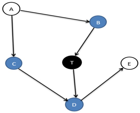
Figure 1.
The Markov blanket of node T.
There are two major approaches for feature selection, i.e., traditional-based and streaming-based. Traditional-based MB discovery (discovery/learning are interchangeable in this article) assumes that all features are readily available from the beginning. This assumption, however, is often violated in real-world applications. For instance, for the problem of detecting Mars crater from high-resolution planetary images [2], it is impracticable to attain the complete feature set, which means to have a near-global coverage of the Martian surface. Several MB discovery algorithms are proposed based on traditional concepts requiring all features and instances to be available before learning. Such algorithms include Incremental Association-Based Markov Blanket (IAMB) [3], HITON-MB (HITON-MB) [4], Simultaneous Markov Blanket (STMB) [5], Balanced Markov Blanket (BAMB) [6], and Efficient and Effective Markov Blanket (EEMB) [7]. Traditional-based MB discovery algorithms do not apply to real-world scenarios, such as users of the famous microblogging website Twitter who yield over 250 million tweets every single day, which includes words and abbreviations [8], personalized recommendations [9], malware scanning [10], and ecological inspection and analysis [11] with the quality of frequent features updates and dynamic space-changing [12]. A fascinating question is whether we should wait long for all features to become accessible before starting the learning process. We need a lot of computational efforts to build such features upfront. This raises an intriguing research challenge about constructing an effective feature selection process without knowing the entire feature space. However, the existing algorithms for Markov blanket discovery commonly assume that all features must be present in advance. Therefore to tackle such issues, streaming feature selection was introduced and applied to many applications such as biology, weather forecasting, transportation, stock markets, clinical research, etc. [8]. Several algorithms based on streaming features (SF) were proposed for real scenarios including Grafting [8], Alpha-investing ( investing) [13], Scalable and Accurate Online Feature Selection (SAOLA) [14], and Online Streaming Feature Selection (OSFS) [15]. However, these algorithms only focus on obtaining PC sets and do not consider the Spouses, which causes them to lose the interpretability by ignoring the causal MB discovery.
Motivated by these observations and issues, this paper presents an Online Streaming Features Selection via Markov Blanket algorithm, based on a statistical conditional independence test. The features are no longer static but flow in one by one and are analyzed as it arrives. A null-conditional test motivated it to address the streaming features, feature relevance analysis to find the true positive PC and Spouses, and feature redundancy analysis to remove the false positive/irrelevant features.
The main contributions of this study are as follows:
- OFSVMB obtains Parent-Child and Spouse feature sets simultaneously and separates them in the MB set;
- OFSVMB reduces the impact of conditionally independent tests errors since it uses fewer conditionally independent tests to learn MB;
- Sensitivity analysis of OFSVMB using three different parameters values concerning the Rate of Instance to analyze the performance with small and large sample sizes;
- Performance evaluation of OFSVMB algorithm on benchmark BN and real-world datasets.
2. Related Work
In traditional MB discovery techniques, features must be present before learning begins. Different algorithms developed for MB learning, which is based on traditional concepts such as Incremental Association-Based Markov Blanket (IAMB) [16], Max-Min Markov Blanket (MMMB) [17], HITON-MB (HITON-MB) [18], Simultaneous Markov Blanket (STMB) [19], Iterative Parent-Child-based MB (IPCMB) [19], Balanced Markov Blanket (BAMB) [6], and Efficient and Effective Markov Blanket (EEMB) [7]. While MB is learning the Parents-Child and Spouses of the target feature, T cannot differentiate by the IAMB [16] algorithm. Additionally, when the sample size of the dataset is not quite large, the IAMB can not faithfully discover the Markov blanket of the target feature T. The Min-Max Markov blanket (MMMB) uses the Divide and Conquer strategy to minimize the size of data samples [17]. It needs to split the dilemma of finding MB into two sub-dilemmas to find the Parents-Child and the Spouses. MMMB has been modified to build HITON-MB, which excludes false-positive features from the Parents-Child set quickly by interleaving the growing and shrinking phases [18]. Under the Markov blanket assumption, MMMB [17] and HITON-MB [18] were conceptually flawed and needed a new mechanism for accurate MB discovery. The Iterative Parent-Child-based search of Markov Blanket (IPCMB) algorithm uses the same PC algorithm as PCMB [19] to identify the PC set and increases the efficiency without losing accuracy [19]. However, the symmetry constraint check makes this algorithm computationally slow. STMB [19] also followed the technique as IPCMB [19] for Parents-Child exploration. However, it consumes more time and avoids symmetry checks.
Moreover, the online feature selection methods receive features one by one dynamically. These methods include grafting [8], Alpha-investing ( investing) [8], Scalable and Accurate Online Feature Selection (SAOLA) [20], and Online Streaming Feature Selection (OSFS) [21]. Grafting was the first algorithm designed by Perkins and Theiler. It attempts the streaming features selection technique, which is a stage-wise technique for gradient descent. Alpha-investing used p-value and threshold to control the feature selection process and decide to select relevant features and remove redundant ones [8]. The benefit of alpha-investing is to handle features sets of unknown sizes even up to infinity, but it fails to investigate redundant features, causing an unpredictable and low prediction accuracy. SAOLA [20] examines two features simultaneously and analyzes redundancy under a single scenario. It fails to find an optimum relevance threshold value to remove all redundant features. In contrast, OSFS [21] removes unnecessary features which are not relevant/associated with the target feature, T, using conditional independence. It uses two steps to achieve the Parents-Child relevant to the target feature T. The first step analyzes the online relevance, and the second step analyzes online redundancy. It identifies the approximate MB without Spouses. The methods of online feature selection such as Alpha-investing, SAOLA, and OSFS only identify Parents-Child (PC) features and avoid the Spouses (SP) and the causality neglect by these algorithms. Based on online feature selection and causality, the Causal Discovery From Streaming Feature (CDFSF) is used [22]. The symmetric Causal Discovery From Streaming Feature (S-CDFSF) [22] is developed, which uses conditional independence test to identify the relevant features of the target feature, T, based on streaming, which belongs to the Parents-Child and Spouses.
3. Preliminaries
In this segment, the MB discovery through streaming features is defined. In addition, the specific aspects are discussed in detail. Table 1 summarized the notations used in this paper based on the new definitions.

Table 1.
Summary of Notation.
Definition 1 (Streaming Features [15]). Involves a feature vector that streams in one by one over time while a number of training samples remain constant.
Definition 2 (Conditional Independence [6]). Feature (variable) is conditionally independent of feature (variable) given S, if and only if .
Definition 3 (Strong relevant [23]). A feature is strongly relevant to the target feature T, if and only if .
Definition 4 (Irrelevant [23]). A feature is irrelevant to a target feature T, if and only if it is .
Definition 5 (Redundant [24]). A feature is redundant to the target variable T, if and only if it is weakly relevant to target variable T and has a Markov blanket, , then it is a subset of the Markov blanket of .
Definition 6 (Faith-fullness Condition [25]). G denotes a Bayesian network, and P represents a joint probability distribution through feature set R. So, G is devoted to P if P captures all. Only the conditional independence is among features in G.
Definition 7 (V-structure [26]). If there is no an arrow between feature (variable) and and feature (variable) , and feature (variable) has two incoming arrows from and , respectively, then , , and form a V-structure .
Definition 8 (D-Separation [26]). A path D between a feature (variable) and feature (variable) is D-separated by set of features (variables) S, if and only if:
- D includes a chain such that the middle one features is in S.
- D includes a collider such that the middle one feature is not in S and none of successors are in S.
A feature set S is said to be D-separated and , if and only if S jammed each path D from a feature to a feature .
Theorem 1.
In a faithful Bayesian Network, an MB of the target feature T, , in a set R is an optimal set of features, composed of Parents, Children, and Spouses. All other features are not conditionally dependent of target feature T given , , s.t. .
4. Online Feature Selection via Markov Blanket
This section presents the proposed algorithm for implementing the framework for feature selection with streaming features called Online features selection via a Markov blanket (OFSVMB).
4.1. Framework of OFSVMB
The framework of the Online Feature Selection via Markov blanket is shown in Table 2. Two conditional tests are used to check the association between features. The first is a statistical test (for discrete data) and the second is the statistical Fisher’s z-test (for continuous data). = (Equal(=) sign means they are same in this article) denotes a conditional independence test between a feature and the target feature (variable) T, given a subset S. While = represents a conditional dependence test between a feature and the target feature T, given a subset S.
Table 2.
The OFSVMB framework.
For a new incoming feature, the OFSVMB algorithm performs the Null conditional independence analysis [26], relevance analysis, and redundancy analysis. The pseudocode of OFSVMB is shown in Algorithm 1. In Algorithm 1 RecogNC, line 5 performs null conditional independence using Proposition 1 to check the dependency between feature and target feature T. If is dependent on target feature T, then add to ; otherwise, add it to non_pc.
Proposition 1.
Using null conditional independence, check the feature relevancy or irrelevancy with target feature T.
Proof of Proposition 1.
Assuming that and , the following hold:
□
Therefore, represents that and are not relevant to each other.
Through the relevancy analysis based on Proposition 2, the OFSVMB analyzes features and adds them to the candidate Parents-Child set and the candidate Spouse set , which are the candidate set of the Parents-Child and Spouse set. If feature is related to the target feature T given , it is added to ; otherwise, it is removed from and added to non_pc.
Furthermore, it also analyzes whether is a candidate spouse from the non_pc set. For example, if feature non_pc, the conditional feature set that causes and target independent variable T is the . If there exists a feature , is related to target variable T under the condition of union N, then is added to the as mentioned in Algorithm 1.
Proposition 2.
A current feature arrived at time t, and T is a target feature. If , i.e., , then .
Proof.
The proof is as follows: If , if feature is related to target feature T under R condition by Theorem 1, then add to . □
Based on Theorem 2 and Proposition 3, using the redundancy analysis, the OFSVMB removes false-positive features separately from the candidate Parent-Child set and the candidate Spouse set , which are the candidate sets of the Parents-Child and Spouse set. However, it also looks for non-MB descendant features in and discards them if they have been through Theorem 2, which makes the OFSVMB different from the other existing algorithms. Removing false positive Spouses through redundant analysis if , if is not dependent to the target feature (variable) T, giving subset S, then is removed from . By removing the irrelevant Spouse such that and , if E is not relevant to target feature T under the condition of , then E is removed from .
Theorem 2.
(PC recognizes false-positives): Only successors of the target T, standing for , make up false-positives .
Proof.
is composed of a whole PC and a few false positives. We show that . is a candidate super-set of all true positive PCs because it should hold the true positive PCs. After an exhaustive search for the PC set, the entire parents set of target T is represented by . According to Definition 5, all non-successor nodes (features) are independent of target T provided . is any non-descendant node if is any non-successor nodes (feature). As a result, f will be omitted from due to the Markov condition . □
Proposition 3.
(Remove false-positives from a Spouse). In a BN, R is a feature set, assuming that is neighboring to , is neighboring to T, and is not neighboring to T (e.g, ). However, once feature M enters , for any existing feature X in , , , then X is a false-positives and removed from .
Proof of Proposition 3.
V-structure illustrates that if is target T’s Spouse and is the mutual Child, there occurs a subset so that features X and T are independent given feature S. Still, they are dependent given . If there is another feature, M exists to block the path between and . M has a direct effect on that is not satisfied by V-structure , so in this condition, X is removed from and is considered as a false-positives Spouse. □
4.2. The Proposed OFSVMB Algorithm and Analysis
This paper segment explains the proposed algorithm for Online Feature Selection via Markov blanket, given in Algorithm 1. The proposed algorithm can derive the by deleting all redundant features. The OFSVMB algorithm based on null-conditional independence test, relevance analysis, and redundant analysis. First, the null-conditional independence [26] (line 5) of Algorithm 1 is used to tackle the streaming feature. It analyze the new feature arrived at time . If is dependent of target T given empty set, (the empty set is equal to ⌀), then include feature to ; otherwise, add to non_pc. After null conditional independence analysis, check if either feature is a true positive (line 6–9) given subset S. If it is not a true positive, remove from (line 10); otherwise, analyze whether it is a candidate Spouse (line 11–19).
| Algorithm 1 OFSVMB. |
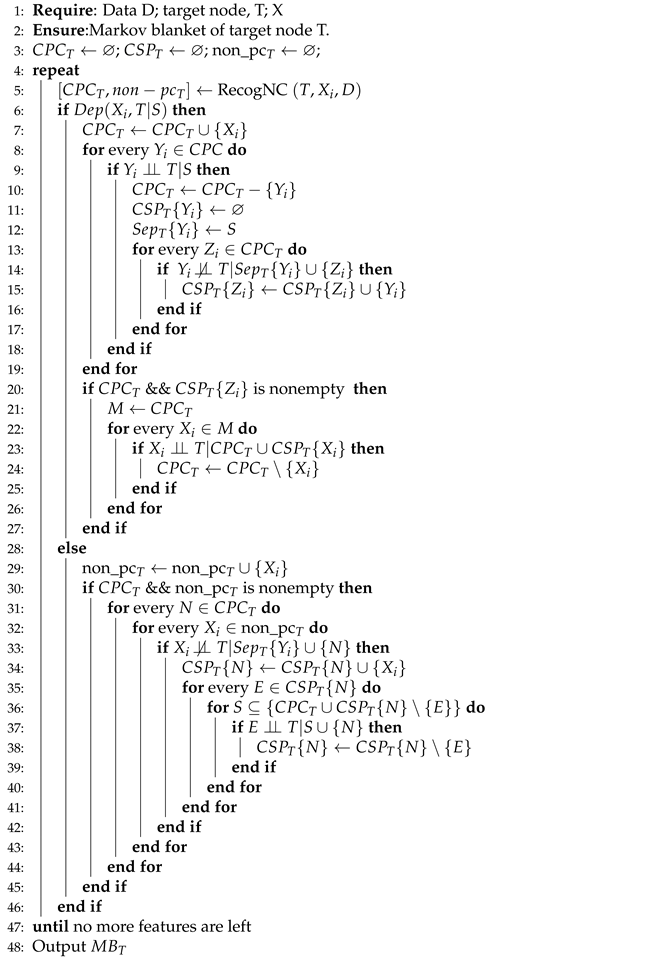 |
OFSVMB then checks non-MB successors in the that may have several pathways to the target variable T. If and T are independent, is removed from the (line 24). Algorithm 1 finds the Parents-Child (line 5–10) and computes the Spouses from the non_pc set that is discarded during the null-conditional independence step (line 5) and from false-positive PC (line 6–10).
Moreover, after checking the conditional independence test at (line 6), if the feature is not dependent on target feature T, it comes to (line 29), to identify the spouse from the non_pc set. If , include the (line 31–34). Through redundant analysis (line 35–45) check whether the selected spouse is redundant, if yes, then discard the false positive/redundant feature from .
4.3. Statistical Conditional Independence Terminology in OFSVMB
The conditional independence test is used to classify irrelevant and redundant features [15], denoted by the notations and in Algorithm 1. The test, equivalent to the test (discrete data), and Fisher’s z-test are used.
4.3.1. Statistical Test for Discrete Data
The with three features (variables), , and , set as the number of checks satisfying , and in a dataset. , and are all described in the same way. If and are conditionally not dependent given , thus, in Equation (1) below, the test is shown:
With sufficient degrees of freedom, is asymptotically distributed as . In general, when checking the conditional independence of and given S, the amount of degrees of freedom used during the test is measured as:
where, in Equation (2), represents the number of distinct values of .
4.3.2. Statistical Fisher’s z-Test for Continuous Data
Fisher’s z-test, on the other hand, calculates the degree of correlation between features as given in Equation (3). After the feature subset S is provided, the partial correlation coefficient between the feature and the target variable T is expressed in the Gaussian distribution [14]:
Under the null hypothesis of conditional independence between the feature and the target variable T of the current feature subset S, , according to Fisher’s z-test. Assume that is a given level of significance and is the p-value obtained by Fisher’s z-test.
Supposing , and target variable T are not related to each other when the subset S is given, according to the null hypothesis of the conditional independence of and target variable T. If , then and target variable T are both relevant.
4.4. Correctness of OFSVMB
OFSVMB produces the MB of the target feature T truly and accurately, under the faithful assumption. According to Theorem 1, in the beginning, OFSVMB finds true positive or relevant features which belong to the . It is a candidate Parents-Child set of target feature T using null-conditional independence and adds them in the candidate parent child (CPC) set, e.g., . In contrast, add the false positive or redundant feature in the non-Parents-Child set (line 5). Then, in the candidate Parents-Child (CPC) set, e.g., , OFSVMB searches for a false positive or redundant feature and discards it from the candidate parent-child (CPC) set (line 9) and (line 10). The contains all relevant features dependent on target feature T given any subset .
Additionally, OFSVMB finds the Spouse (line 13–19) of target T at the same time as looking for a redundant feature in the set. Non-MB successors in are discarded by conditioning on the true positive Spouse in , combined with the true positive PC in in the joint set and (line 20–27). Suppose the feature (line 6) is independent of target feature T, so the OFSVMB considers searching Spouse from the non_pc set (line 29–34) and simultaneously removes the redundant feature from through redundant analysis (line 35–38). At last, if there is no feature left, OFSVMB finds the Markov blanket (MB) of target feature T at (line 48), which is the union of true positive = and true positive = .
4.5. Time Complexity Analysis
The time complexity, as presented in Table 3 of the state-of-the-art MB discovery algorithms, counts on how many CI tests have been used in the algorithm. OFSVMB identifies the MB of target feature T through online relevance and redundancy analysis. It is assumed that R represents the total number of features that appeared with time t, where is the number of features relevant to target feature T in R. The remaining number of features in R, not relevant to target T, is represented by . represents the Candidate Parents-Child set, and represents a subset of the Spouses of target T with regards to target T’s child . When the feature appears at time t, the OFSVMB time complexity is explained below: The null-conditional independence has a time complexity of . The Parents-Child identification takes and the discovery of Candidate Spouses is , where k is the maximum limit of a conditioning set that might increase. The OFSVMB is based on streaming discard redundant features in the streaming scenario, and both and become smaller. The approximate time complexity of the proposed OFSVMB algorithm is , where C is the is equal to and . The OFSVMB is somehow more efficient than the state-of-the-art because it handles features in real-time scenarios.
Table 3.
Time complexity of Markov blanket (MB) discovery Algorithm.
The proposed OFSVMB and EEMB accuracy are comparable. However, OFSVMB performs the streaming feature selection where features come one by one inflow, so removing the redundant features from and jointly takes a few CI tests. The STMB uses a backward strategy during PC learning and identifies the separated PC set from all other subsets of R at any repetition. It makes the STMB slower than the proposed OFSVMB algorithm, as presented in Table 3.
5. Results and Discussion
In this segment, the results of the proposed OFSVMB are discussed in detail. The results are conducted through extensive experiments and comparing them with the traditional-based MB discovery algorithms such as Iterative Associative Markov Blanket (IAMB), Simultaneous MB (STMB), HITON-MB (HITON-MB), Balanced Markov Blanket (BAMB), an Efficient and Effective MB discovery (EEMB), and streaming-based algorithms such as Alpha-investing (-investing), Scalable and Accurate Online Feature Selection (SAOLA), and Online Streaming Feature Selection (OSFS).
5.1. Datasets and Experiment Setup
The experimental results are computed on 9 benchmark BN datasets (https://pages.mtu.edu/lebrown/supplements/mmhc_paper/mmhc_index.html, accessed on 1 July 2021) of small and large sample-size, as shown in Table 4, and 14 real-world feature selection datasets as shown in Table 5. The real-world datasets are selected from different domains, such as sets from the UCI machine learning repository [27]; frequently studied public microarray (wdbc) [28], ionoshpere, colon, arcene, leukemia, and madelon are from the NIPS 2003 feature selection competition [29]; lung and medical belongs to biomedical [30]; lymphoma, reged1, and marti1 [31,32]; and prostate-GE and sido0 [33,34].
Table 4.
Outline of the benchmark BN datasets.
Table 5.
Outline of the real-world datasets.
The OFSVMB algorithm is implemented in Matlab R2017b. All the experimental work is conducted on Windows 10 with an Intel Core i5-6500U with 8 GB RAM. The two conditional independence (CI) tests, including the test (for discrete data) and the Fisher’s z-test (for continuous data) with the significance levels of 0.01 and 0.05 are used.
5.2. Evaluation Metrics
The performance of the proposed OFSVMB algorithm is evaluated using three evaluation metrics on the benchmark BN datasets. The evaluation metrics are as follows:
- Precision: The number of true positives in an algorithm’s output (e.g., features that belong to the true MB of a target feature in a DAG) divided by the number of features in the algorithm’s output yields this metric.
- Recall: This metric is calculated by dividing the number of true positives in the output by the number of true positives (the true MB of a target feature in a DAG).
- F1 = : The harmonic mean of the precision and recall is used to calculate the F1 score. In the best-case scenario, F1 = 1 if precision and recall are both excellent. In the worst-case scenario, F1 = 0.
Each benchmark BNs contains two groups of sample size, i.e., 500 and 5000.
Results and Discussion on Benchmark BN
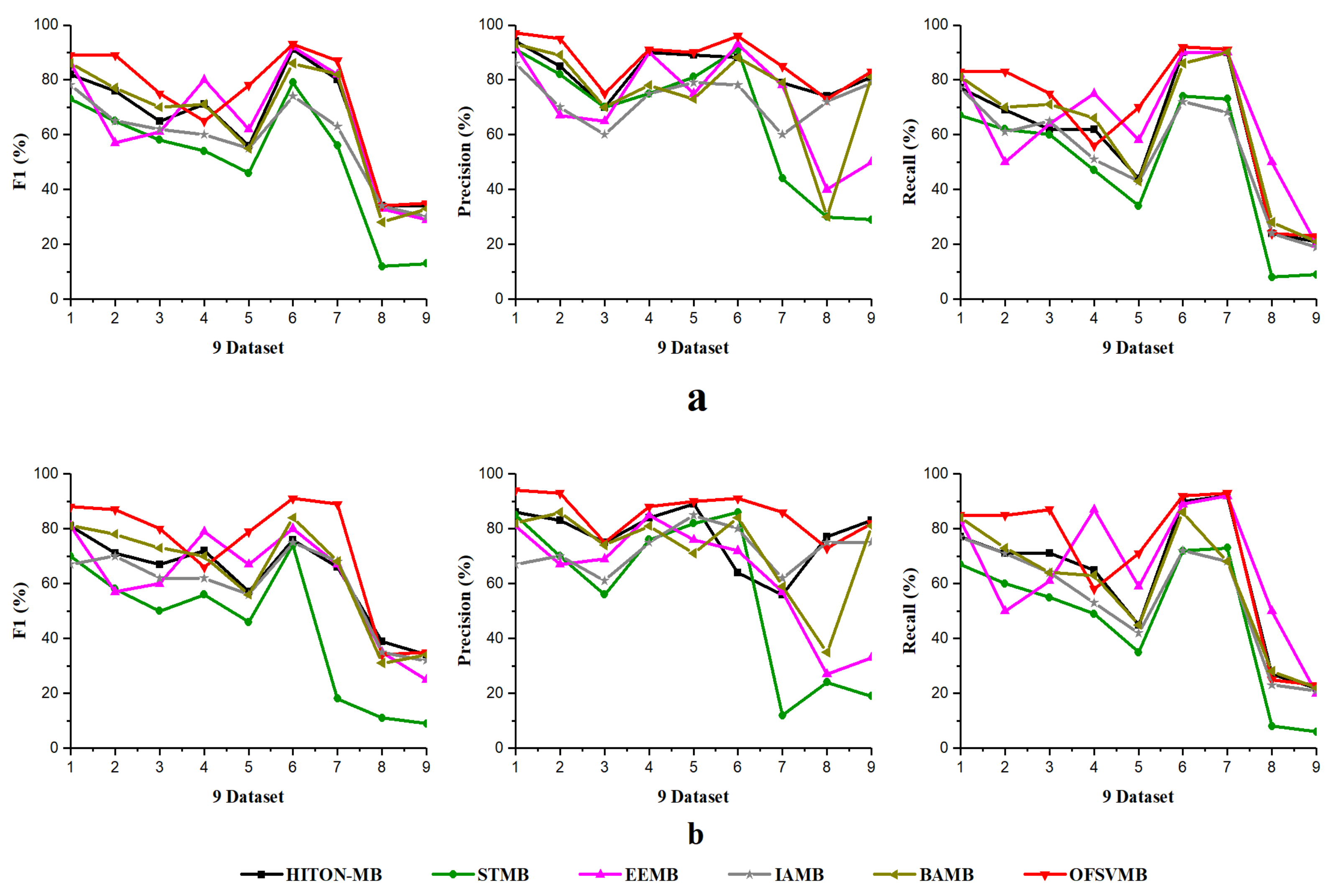
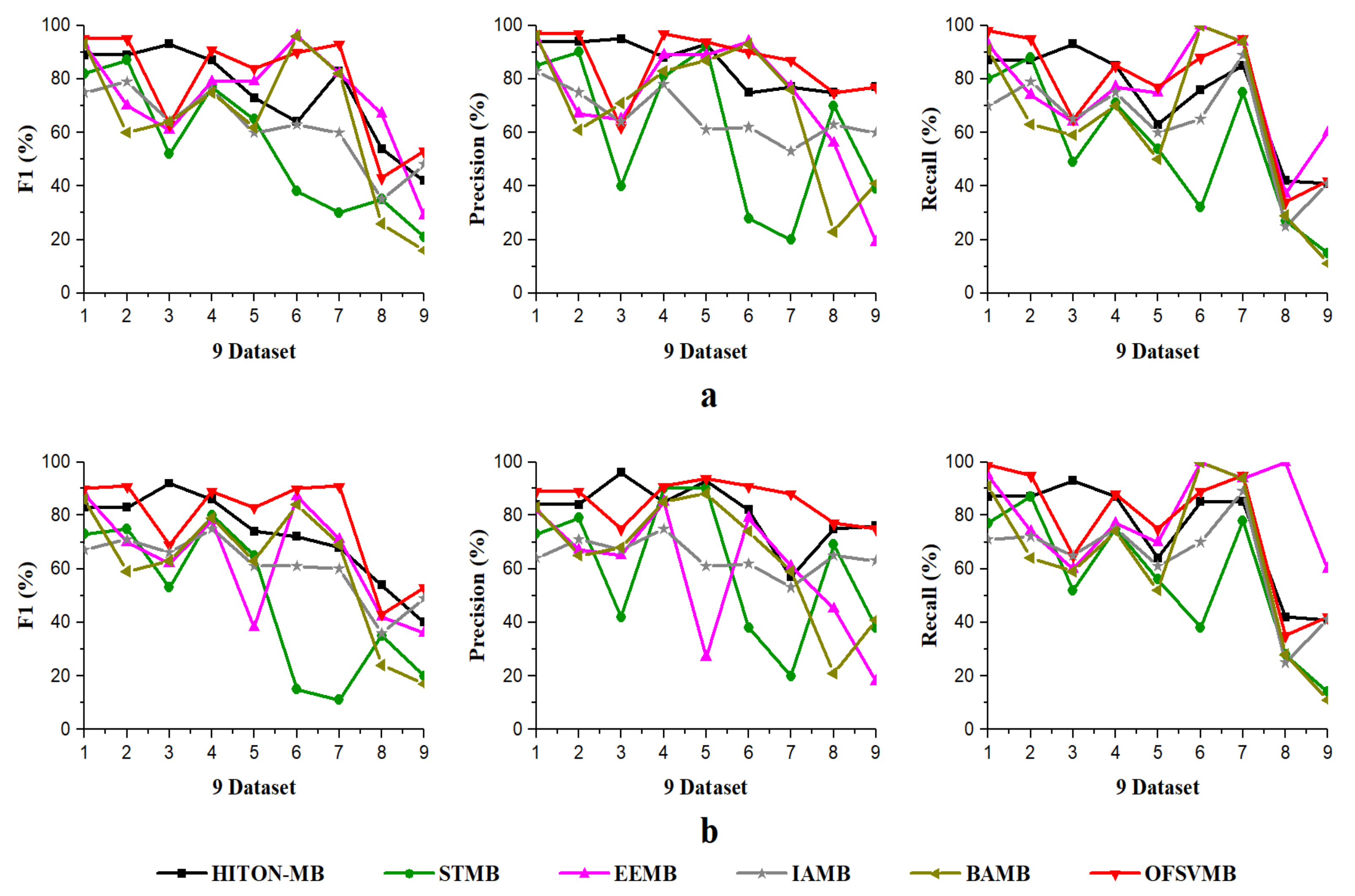
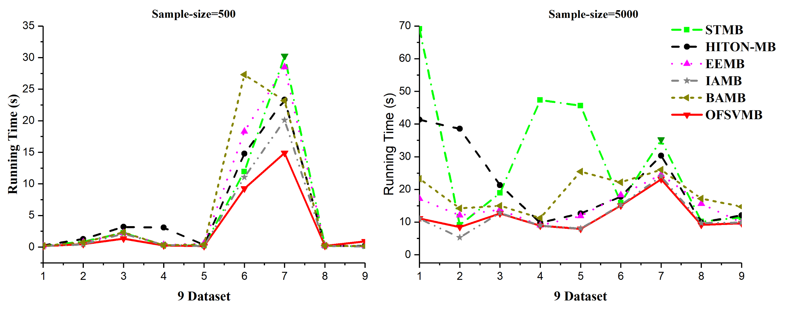
The efficiency and efficacy of the proposed OFSVMB algorithm is computed and compared with other state-of-the-art traditional-based MB discovery algorithms, such as IAMB, STMB, HITON-MB, BAMB, and EEMB, on 9 benchmark BN datasets. The F1, precision, recall, and running time in seconds of OFSVMB and other state-of-the-art are shown in Table 6 for 500 samples and Table 7 for 5000 samples. The sign “/” represents the separation of significant level, e.g., on the left side the and on the right side the , where is the significant level. The F1, precision, and recall of sample sizes 500 and 5000 (a) shows significance levels of 0.01 and (b) shows significance levels of 0.05 in Figure 2 and Figure 3, respectively. Moreover, Figure 4 shows the running time of OFSVMB and five other state-of-the-art algorithms with different sample sizes. In the figures, the x-axis are denoted as the number of datasets (see Table 4), and the y-axis represent the F1, precision, and recall, together with running time, respectively.
Table 6.
F1, Precision, Recall, and Running time (s) on small and large-size benchmark BN datasets with sample size = 500.
Table 7.
F1, Precision, Recall, and Running time (s) on small and large-size benchmark BN datasets with sample size = 5000.

Figure 2.
F1, Precision, Recall using 9 benchmark BN datasets: (a) significance level = 0.01; (b) significance level = 0.05 with sample size of 500.
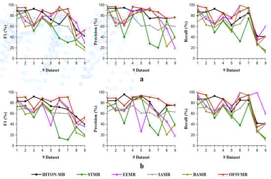
Figure 3.
Precision, Recall, F1 using 9 benchmark BN datasets: (a) significance level = 0.01; (b) significance level = 0.05, with sample size of 5000.
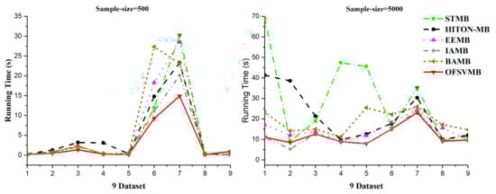
Figure 4.
Running time on 9 benchmark BNs datasets, sample sizes of 500 and 5000.
According to Table 6, OFSVMB is the most accurate and fastest algorithm among the other five state-of-the-art algorithms because it is based on streaming features, which compute the features in an online manner. Meanwhile, on Child, Child3, and Insurance datasets with a sample size of 500 and significance levels of 0.01 and 0.05, OFSVMB is accurate in terms of F1, precision, and recall compared to IAMB, STMB, HITON-MB, BAMB, and EEMB, while faster than STMB, HITON-MB, BAMB, and EEMB. STMB and BAMB do not perform the symmetry check, but they must conduct an exhaustive subset analysis for the PC learning, making these two algorithms relatively slow and inefficient. The OFSVMB is slower than IAMB on Child and Child3 datasets because in each iteration, IAMB uses the entire set of presently selected features as conditioning set to identify whether or not to add or remove a feature from the currently selected features. IAMB is computationally efficient on datasets with small sample sizes, as presented in Table 6 in bold and shown in Figure 2a,b and Figure 4. On Child10 datasets, the OFSVMB is faster than other state-of-the-art algorithms, and IAMB is the second fastest, as shown in Table 6 in bold and shown in Figure 2a,b and the running time in Figure 4. Moreover, on the Child10 dataset, the HITON-MB’s accuracy is comparable with the OFSVMB in terms of precision with a significance level of 0.05, as shown in Table 6 in bold.
On the Alarm10 dataset with a sample size of 500, the EEMB is more accurate in terms of F1 and recall than the OFSVMB, IAMB, STMB, HITON-MB, and BAMB. At the same time, the OFSVMB is accurate than EEMB in terms of precision and the running time is faster as well, as presented in Table 6 in bold and shown in Figure 2a,b and Figure 4. On extensive datasets such as Pig and Gene with a sample size of 500 using significance levels of 0.01 and 0.05, OFSVMB is accurate in terms of F1, precision, and recall compared to its rivals, as shown in Figure 2a,b, while it is faster than the state-of-the-art as presented in Table 6 in bold and in Figure 4. In a dense dataset such as Barley, the HITON-MB is more accurate because HITON-MB locates the target’s Spouses, and must find the PC of each feature in the target’s discovered PC set. This method drastically reduces the number of sample data required and increases MB discovery performance, especially when dealing with high-dimensional and small data samples. When the size of the PC set of the features within the target’s PC set is enormous, therefore, this type of technique is computationally costly. The HITON-MB accuracy is higher in terms of F1 and precision than IAMB, STMB, BAMB, EEMB, and OFSVMB, but at a significance level of 0.01, the OFSVMB has comparable accuracy with HITON-MB in terms of F1. Moreover, in terms of recall, the EEMB has higher accuracy than IAMB, STMB, HITON-MB, BAMB, and OFSVMB, but the OFSVMB has higher running time than others, as shown in Table 6 in bold and Figure 2a,b and Figure 4. On Mildew, the OFSVMB shows higher accuracy than other algorithms. However, HITON-MB is more accurate than the OFSVMB and the others such as IAMB, STMB, BAMB, and EEMB at a significance level of 0.05 in terms of precision. In contrast, at a significance level of 0.01, the OFSVMB is more accurate than HITON-MB, as shown in Table 6. The OFSVMB on the Mildew dataset runs faster than the state-of-the-art as presented in Table 6 in bold and shown in Figure 2a,b and Figure 4.
On small Child and Child3 datasets with a sample size of 5000 using significance levels of 0.01 and 0.05, OFSVMB is more accurate in terms of F1, precision, and recall compared to others, as presented in Table 7 in bold and shown in Figure 3a,b. However, on the Child dataset, the OFSVMB runs faster than the HITON-MB, STMB, BAMB, and EEMB but slower than IAMB. While on the Child3 dataset, the IAMB runs faster than the OFSVMB and the other four algorithms as shown in Table 7, and the running time is shown in Figure 4. On the Child10 dataset with a sample size of 5000, HITON-MB outperforms on OFSVMB, IAMB, STMB, BAMB, and EEMB in terms of F1, precision, and recall, while OFSVMB is run faster than the other 5 algorithms as shown in Table 7 in bold. Figure 3a,b shows the accuracy of OFSVMB and other algorithms, while the running time is given in Figure 4. On the Alarm10, Insurance datasets with a sample size of 5000, OFSVMB is more accurate than IAMB, STMB, HITON-MB, BAMB, and EEMB in terms of F1, precision, and recall as shown in Table 7 in bold and in Figure 3a,b. Meanwhile, OFSVMB shows higher accuracy and better running time than others, as shown in Figure 4. On a large-size dataset with a sample size of 5000, such as the Pig, the BAMB and EEMB are more accurate in terms of F1 and precision at a significance level of 0.01 and for recall at significance levels of 0.01 and 0.05, as shown in Table 7 in bold and in Figure 3a,b. The OFSVMB is more accurate in terms of F1 and precision at significance levels of 0.05 and runs faster than its rivals as shown in Figure 4. Moreover, on an extensive Gene dataset, the OFSVMB is still more accurate and runs faster than other state-of-the-art algorithms as shown in Table 7 in bold and in Figure 3a,b, and the running time is shown in Figure 4.
In a dense dataset with a sample size of 5000, such as the Barley, the EEMB is more accurate in terms of F1 and recall at a significant level of 0.01 and 0.05, as shown in Table 7 in bold and in Figure 3a,b. Still, OFSVMB is more accurate in terms of precision at a significance level of 0.01 and 0.05 than EEMB and runs faster than others, as shown in Figure 4. While on the Mildew dataset, the OFSVMB is more accurate than IAMB, STMB, BAMB, and EEMB. The HITON-MB is more accurate than OFSVMB in terms of precision at a significance level of 0.05, while comparable accuracy in terms of precision at a significance level of 0.01, as shown in Table 7 in bold and in Figure 3a,b and runs faster than other algorithms as shown in Figure 4.
5.3. Evaluation Classifiers
The number of selected features and the prediction accuracy of OFSVMB on 14 real-world datasets with low to high dimensionality is conducted using 12 classifiers including C1 = Coarse Gaussian SVM, C2 = Coarse KNN, C3 = Coarse Tree, C4 = Cosine KNN, C5 = Fine Gaussian SVM, C6 = Fine Tree, C7 = Linear Discriminant, C8 = Linear SVM, C9 = Medium KNN, C10 = Medium Tree, C11 = Subspace Discriminant, and C12 = Subspace KNN, where C standards for classifier and saving space in Table 8, Table 9, Table 10 and Table 11, the abbreviation is used with numbers. For all the datasets, cross-validation is used 10-fold to prevent bias in error estimation. Moreover, the selected number of features and running time in seconds are also reported to show the efficiency of the algorithms.
Table 8.
Comparison of prediction accuracy under C1–C6 classifiers at significance level = 0.01.
Table 9.
Comparison of prediction accuracy under C7–C12 classifiers at significance level = 0.01.
Table 10.
Comparison of mean prediction accuracy under C1–C6 classifiers at significance level = 0.01.
Table 11.
Comparison of mean prediction accuracy under C7–C12 classifiers at significance level = 0.01.
Results and Discussion on Real-World Dataset
This segment shows the comparison of selected features, prediction accuracy, and efficiency of the OFSVMB algorithm with other state-of-the-art streaming-based algorithms, such as Alpha-investing, SAOLA, and OSFS, on 14 real-world datasets with a significance level of 0.01. The following Table 8, Table 9, Table 10, Table 11 and Table 12 describe the prediction accuracy, mean prediction accuracy based on 12 classifiers, and the number of selected features and running time in seconds.
Table 12.
#F (number of selected features) and running time (s) at significance level = 0.01.
Figure 5 shows the prediction accuracy of the algorithms based on 12 classifiers where the x-axis denotes the dataset, and the y-axis represents the prediction accuracy. In contrast, Figure 6 shows the running time in seconds of the algorithms. The sign “−” denotes that the algorithm fails to select any number of features in the corresponding dataset and takes longer. The better outcomes are underlined in bold text, presented in the following Table 8, Table 9, Table 10, Table 11 and Table 12.
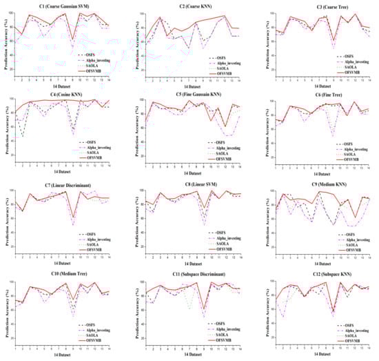
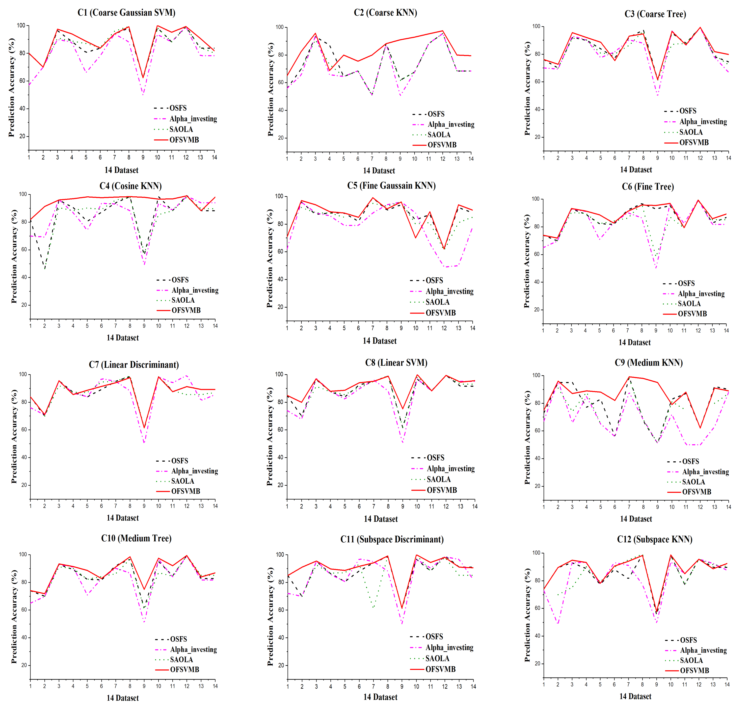
Figure 5.
Prediction Accuracy in the 14 real-world datasets under 12 classifiers.

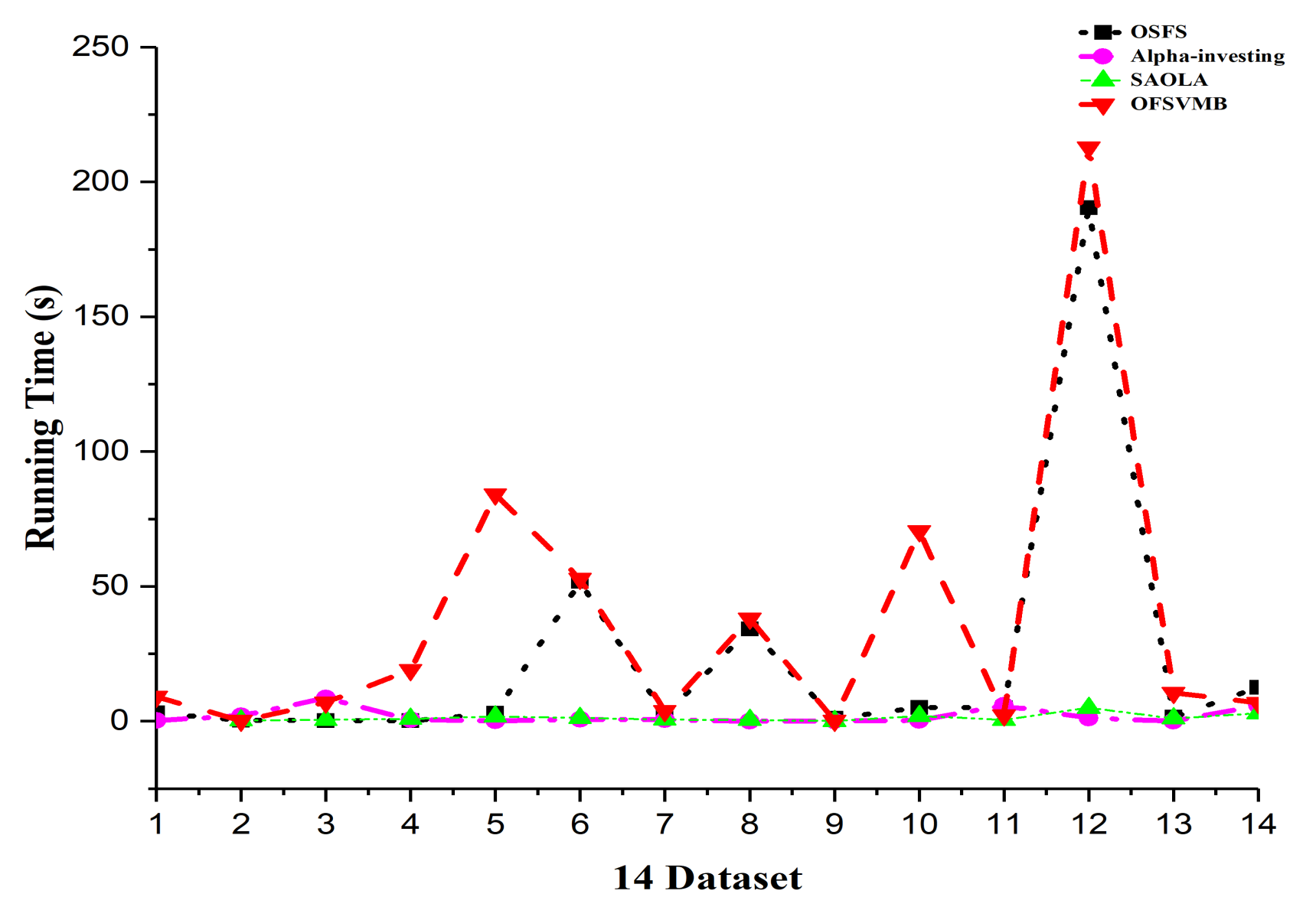
Figure 6.
Running time in the 14 real-world datasets.
Table 8 and Table 9 describe the prediction accuracy of OFSVMB against OSFS, Alpha-investing, and SAOLA using 12 classifiers. As described in the tables, OFSVMB performs better than the other algorithms on most datasets. Its mean prediction accuracy is higher than others using the 12 classifiers as shown in Table 10 and Table 11. The OFSVMB searches for PC and Spouse of the target feature T. In contrast, the OSFS, Alpha-investing, and SAOLA only search for PC and ignore the Spouse set of the target feature T, which causes them to lose the interpretability.
On the arcene dataset, SAOLA fails to obtain any features, as shown in Table 8 and Table 9. OSFS and Alpha-investing have comparable accuracy with OFSVMB on very few datasets. OFSVMB somehow includes false positives, not worse than its rivals on real-world feature selection datasets. From Figure 5, the OFSVMB has better prediction accuracy compared with other algorithms on many datasets under 12 classifiers. Table 12 describes the number of selected features and the running time of the algorithms. Alpha-investing selects more features on many datasets because it does not re-evaluate the redundant features, making it ineffective but time-efficient. The OSFS selects fewer features than Alpha-investing and SAOLA and OFSVMB; when the new feature arrives, the OSFS first checks the relevancy, and then the arrived features’ redundancy, which improves accuracy against Alpha-investing and SAOLA, and selects fewer features.
The running time of OSFS is slower than Alpha-investing and SAOLA on many datasets because it considers features repeatedly to add or remove them from the feature set. The OFSVMB selects many features from many datasets and causes its running time to be slower than other algorithms, as shown in Figure 6. The OFSVMB searches for the PC and Spouse of the target feature T, while OSFS, Alpha-investing, and SAOLA only search the PC set of the target feature T.
5.4. Sensitivity Analysis
The OFSVMB algorithm is governed by (Alpha and significance level are similar) and . We conducted a sensitivity analysis to investigate the effect of parameter values on the model’s accuracy. This section provides the details of sensitivity experiments. Concerning different parameters, including values and with different Rate of Instance , the analysis is practiced on six real-world feature selection datasets, where the Rate of Instance is the subset of instances from the dataset. We choose three values of such as concerning three different values of the such as .
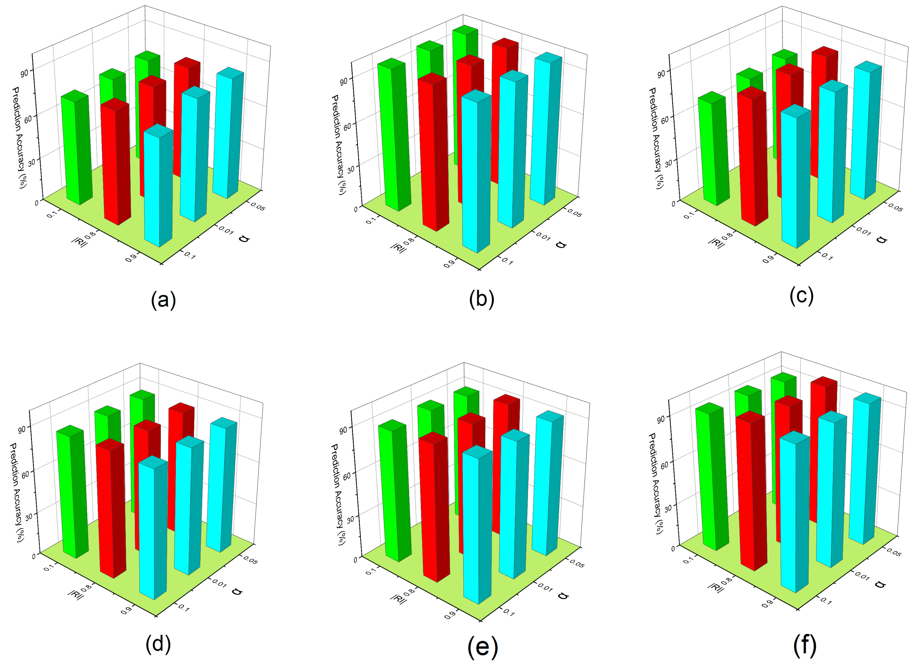
The parameter determines how well the reconstruction function preserves the original, observable feature’s values. The = is used to see the effect of OFSVMB prediction accuracy. In contrast, investigating = can keep important features along the instance to affect the prediction accuracy of the OFSVMB. In Figure 7, the x-axis represents the Rate of Instance , the y-axis represents parameter , and the z-axis represents the prediction accuracy (%) on six real-world datasets including (a) spect, (b) sylva, (c) madelon, (d) marti1, (e) ionosphere, and (f) reged1. These six datasets contain small and large sample sizes and sparse data.

Figure 7.
Prediction accuracy of OFSVMB with respect to different and on 6 real-world datasets: (a) spect, (b) sylva, (c) madelon, (d) marti1, (e) ionosphere, (f) reged1.
From the results given in Figure 7c, we observe that when is fixed with different values, the prediction accuracy of the OFSVMB algorithm increases for = 0.8 and 0.9. For some datasets given in Figure 7b,f, when the = 0.1, it can still keep the important feature along with instances and increase the prediction accuracy. We observe that the most optimal values of parameter are 0.01 and 0.05, and under these values with different , the prediction accuracy of OFSVMB is higher. Still, the parameter = 0.1 with different also has an optimal contribution to the given six datasets regarding prediction accuracy. Thus, such an empirical value can be adopted in practice for future methods based on the statistical conditional independence test. These observations conclude that the OFSVMB is more accurate in selecting the optimal features regarding different with different .
6. Conclusions
This paper proposes an Online Feature Selection via Markov Blanket (OFSVMB) algorithm that uses conditional independence and Fisher’s z-tests to find the MB based on streaming features. Once a feature is included in the PC and SP sets using online relevance analysis, it examines and checks for a true or false-positive feature using the online redundant analysis. OFSVMB tries to make the candidate features set of both PC and SP as small as possible, reducing the number of conditional independence tests. The proposed OFSVMB jointly identifies the Parents-Child and Spouse and separates them in streaming. The evaluation metrics such as F1, precision, and recall are used for evaluating the proposed algorithm on benchmark BN datasets and real-world datasets with 12 classifiers. Additionally, it also obtains the MB set with the highest accuracy. The results demonstrate that the OFSVMB is better than the traditional-based MB discovery algorithms such as IAMB, STMB, HITON-MB, BAMB, and EEMB on most benchmark BN datasets such as Child, Child3, Insurance, Pig, Gene with a sample size of 500 and Child3, Alarm10, Insurance, Gene, and Mildew with a sample size of 5000 with significance levels of 0.01 and 0.05. The OFSVMB also performs better on mean prediction accuracy regarding real-world datasets as compared to other streaming-based algorithms such as OSFS, Alpha-investing, and SAOLA using 12 classifiers including Fine Tree, Medium Tree, Coarse Tree, Linear Discriminant, Linear SVM, Fine Gaussian SVM, Coarse Gaussian SVM, Medium KNN, Coarse KNN, Cosine KNN, Subspace Discriminant, Subspace KNN. Furthermore, Searching feature strategies including the PC and Spouses of OFSVMB makes it a little time-consuming than OSFS, Alpha-investing, and SAOLA because these algorithms only search for the PC feature set and ignore the Spouses. OFSVMB is based on MB discovery, so it considers both PC and Spouses of the target feature T. In addition, the sensitivity analysis using two parameters and Rate of Instance also shows the OFSVMB performs better.
On a large and dense network with many features, statistical hypothesis-based tests for conditional independence causes performance inconsistency in OFSVMB and reduce accuracy. Using a V-structure cause the OFSVMB running time to be slower against OSFS, Alpha-investing, and SAOLA because Alpha-investing and SAOLA select many features. However, they are still faster than our proposed algorithm.
In future work, we plan to overcome the limitations of the proposed algorithm and extend our work to address the direct causes and effects of obtaining the local causal discovery in the streaming feature of the target variable T using mutual information or Neighborhood mutual information with a combination of conditional independence tests using different structure instead of V-structure. It will help to compute more true positive PCs and Spouses. In addition, the focus will be to improve the accuracy and consistently examine the impact of causal faith-fullness violations in the streaming feature selection.
Author Contributions
Conceptualization, W.K., L.K. and B.B; methodology, software, formal analysis, validation, data curation, writing—original draft preparation, W.K. and L.K.; investigation, resources, supervision, project administration, funding acquisition, L.K.; writing—review and editing, visualization, W.K., B.B., L.W. and H.Y. All authors have read and agreed to the published version of the manuscript.
Funding
This research received no external funding.
Institutional Review Board Statement
Not applicable.
Informed Consent Statement
Not applicable.
Data Availability Statement
Not applicable.
Conflicts of Interest
There is no conflict of interest.
Abbreviations
The following abbreviations are used in this manuscript:
| MB | Markov Blanket |
| BN | Bayesian Network |
| PC | Parents-Child |
| SP | Spouse |
| SF | Streaming Feature |
References
- Wu, D.; He, Y.; Luo, X.; Zhou, M. A Latent Factor Analysis-Based Approach to Online Sparse Streaming Feature Selection. IEEE Trans. Syst. Man Cybern. Syst. 2021. [Google Scholar] [CrossRef]
- DeLatte, D.; Crites, S.T.; Guttenberg, N.; Yairi, T. Automated crater detection algorithms from a machine learning perspective in the convolutional neural network era. Adv. Space Res. 2019, 64, 1615–1628. [Google Scholar] [CrossRef]
- Tsamardinos, I.; Aliferis, C. Towards Principled Feature Selection: Relevancy, Filters and Wrappers. In Proceedings of the International Workshop on Artificial Intelligence and Statistics, Key West, FL, USA, 3–6 January 2003. [Google Scholar]
- Aliferis, C.; Tsamardinos, I.; Statnikov, A. HITON: A Novel Markov Blanket Algorithm for Optimal Variable Selection. In Annual Symposium Proceedings. AMIA Symposium; AMIA: Bethesda, MD, USA, 2003; pp. 21–25. [Google Scholar]
- Gao, T.; Ji, Q. Efficient Markov Blanket Discovery and Its Application. IEEE Trans. Cybern. 2017, 47, 1169–1179. [Google Scholar] [CrossRef] [PubMed]
- Ling, Z.; Yu, K.; Wang, H.; Liu, L.; Ding, W.; Wu, X. BAMB: A Balanced Markov Blanket Discovery Approach to Feature Selection. ACM Trans. Intell. Syst. Technol. 2019, 10, 52:1–52:25. [Google Scholar] [CrossRef]
- Wang, H.; Ling, Z.; Yu, K.; Wu, X. Towards efficient and effective discovery of Markov blankets for feature selection. Inf. Sci. 2020, 509, 227–242. [Google Scholar] [CrossRef]
- Alnuaimi, N.; Masud, M.; Serhani, M.A.; Zaki, N. Streaming feature selection algorithms for big data: A survey. Appl. Comput. Inform. 2020. [Google Scholar] [CrossRef]
- Pan, W.; Chen, L.; Ming, Z. Personalized recommendation with implicit feedback via learning pairwise preferences over item-sets. Knowl. Inf. Syst. 2019, 58, 295–318. [Google Scholar] [CrossRef]
- Yang, S.; Wang, H.; Hu, X. Efficient Local Causal Discovery Based on Markov Blanket. arXiv 2019, arXiv:abs/1910.01288. [Google Scholar]
- Sowmya, R.; Suneetha, K. Data mining with big data. In Proceedings of the 2017 11th International Conference on Intelligent Systems and Control (ISCO), Coimbatore, India, 5–6 January 2017; pp. 246–250. [Google Scholar]
- Boulesnane, A.; Meshoul, S. Effective Streaming Evolutionary Feature Selection Using Dynamic Optimization. In IFIP International Conference on Computational Intelligence and Its Applications; Springer: Berlin, Germany, 2018; pp. 329–340. [Google Scholar]
- Zhou, J.; Foster, D.; Stine, R.; Ungar, L. Streaming feature selection using alpha-investing. In Proceedings of the Eleventh ACM SIGKDD International Conference on Knowledge Discovery in data Mining, Chicago, IL USA, 21–24 August 2005; pp. 384–393. [Google Scholar]
- Yu, K.; Wu, X.; Ding, W.; Pei, J. Scalable and accurate online feature selection for big data. ACM Trans. Knowl. Discov. Data (TKDD) 2016, 11, 1–39. [Google Scholar] [CrossRef]
- Wu, X.; Yu, K.; Ding, W.; Wang, H.; Zhu, X. Online feature selection with streaming features. IEEE Trans. Pattern Anal. Mach. Intell. 2012, 35, 1178–1192. [Google Scholar]
- Yu, K.; Guo, X.; Liu, L.; Li, J.; Wang, H.; Ling, Z.; Wu, X. Causality-based feature selection: Methods and evaluations. ACM Comput. Surv. (CSUR) 2020, 53, 1–36. [Google Scholar] [CrossRef]
- Wu, X.; Jiang, B.; Yu, K.; Chen, H.; Miao, C. Multi-label causal feature selection. Proc. Aaai Conf. Artif. Intell. 2020, 34, 6430–6437. [Google Scholar] [CrossRef]
- Liu, C.; Yang, S.; Yu, K. Markov Boundary Learning With Streaming Data for Supervised Classification. IEEE Access 2020, 8, 102222–102234. [Google Scholar] [CrossRef]
- Ling, Z.; Yu, K.; Wang, H.; Li, L.; Wu, X. Using feature selection for local causal structure learning. IEEE Trans. Emerg. Top. Comput. Intell. 2020, 5, 530–540. [Google Scholar] [CrossRef]
- Zhou, P.; Wang, N.; Zhao, S. Online group streaming feature selection considering feature interaction. Knowl.-Based Syst. 2021, 226, 107157. [Google Scholar] [CrossRef]
- You, D.; Wang, Y.; Xiao, J.; Lin, Y.; Pan, M.; Chen, Z.; Shen, L.; Wu, X. Online Multi-label Streaming Feature Selection with Label Correlation. IEEE Trans. Knowl. Data Eng. 2021. [Google Scholar] [CrossRef]
- Li, L.; Lin, Y.; Zhao, H.; Chen, J.; Li, S. Causality-based online streaming feature selection. In Concurrency and Computation: Practice and Experience; Wiley Online Library: Hoboken, NJ, USA, 2021; p. e6347. [Google Scholar]
- Wang, H.; You, D. Online Streaming Feature Selection via Multi-Conditional Independence and Mutual Information Entropy†. Int. J. Comput. Intell. Syst. 2020, 13, 479–487. [Google Scholar] [CrossRef]
- You, D.; Wu, X.; Shen, L.; He, Y.; Yuan, X.; Chen, Z.; Deng, S.; Ma, C. Online Streaming Feature Selection via Conditional Independence. Appl. Sci. 2018, 8, 2548. [Google Scholar] [CrossRef] [Green Version]
- Spirtes, P.; Glymour, C.; Scheines, R. Causation, prediction, and search. In Causation, Prediction, and Search; Springer: New York, NY, USA, 1993; pp. 238–258. [Google Scholar]
- You, D.; Li, R.; Sun, M.; Ou, X.; Liang, S.; Yuan, F. Online Markov Blanket Discovery With Streaming Features. In Proceedings of the 2020 IEEE International Conference on Knowledge Graph (ICKG), Nanjing, China, 9–11 August 2020; pp. 92–99. [Google Scholar]
- Singh, A.; Kumar, R. Heart Disease Prediction Using Machine Learning Algorithms. In Proceedings of the 2020 International Conference on Electrical and Electronics Engineering (ICE3), Gorakhpur, India, 14–15 February 2020; pp. 452–457. [Google Scholar]
- Shen, Z.; Chen, X.; Garibaldi, J. Performance Optimization of a Fuzzy Entropy Based Feature Selection and Classification Framework. In Proceedings of the 2018 IEEE International Conference on Systems, Man, and Cybernetics (SMC), Miyazaki, Japan, 7–10 October 2021; pp. 1361–1367. [Google Scholar]
- Wu, D.; Luo, X.; Shang, M.; He, Y.; Wang, G.; Wu, X. A data-characteristic-aware latent factor model for web services QoS prediction. IEEE Trans. Knowl. Data Eng. 2020. [Google Scholar] [CrossRef]
- Ucar, M.K.; Nour, M.; Sindi, H.F.; Polat, K. The Effect of Training and Testing Process on Machine Learning in Biomedical Datasets. Math. Probl. Eng. 2020, 2020, 2836236. [Google Scholar] [CrossRef]
- Hu, W.; Fey, M.; Zitnik, M.; Dong, Y.; Ren, H.; Liu, B.; Catasta, M.; Leskovec, J. Open Graph Benchmark: Datasets for Machine Learning on Graphs. arXiv 2020, arXiv:abs/2005.00687. [Google Scholar]
- He, Y.; Wu, B.; Wu, D.; Beyazit, E.; Chen, S.; Wu, X. Toward Mining Capricious Data Streams: A Generative Approach. IEEE Trans. Neural Networks Learn. Syst. 2021, 32, 1228–1240. [Google Scholar] [CrossRef] [PubMed]
- Ge, C.; Zhang, L.; Liao, B. Abstract 5327: KPG-121, a novel CRBN modulator, potently inhibits growth of metastatic castration resistant prostate cancer as a single agent or in combination with androgen receptor signaling inhibitors both in vitro and in vivo. Cancer Res. 2020, 80, 5327. [Google Scholar]
- Caesar, H.; Bankiti, V.; Lang, A.H.; Vora, S.; Liong, V.E.; Xu, Q.; Krishnan, A.; Pan, Y.; Baldan, G.; Beijbom, O. nuScenes: A Multimodal Dataset for Autonomous Driving. In Proceedings of the 2020 IEEE/CVF Conference on Computer Vision and Pattern Recognition (CVPR), Seattle, WA, USA, 13–19 June 2020; pp. 11618–11628. [Google Scholar]

Publisher’s Note: MDPI stays neutral with regard to jurisdictional claims in published maps and institutional affiliations. |
© 2022 by the authors. Licensee MDPI, Basel, Switzerland. This article is an open access article distributed under the terms and conditions of the Creative Commons Attribution (CC BY) license (https://creativecommons.org/licenses/by/4.0/).