Reasoning Method Based on Intervals with Symmetric Truncated Normal Density

Abstract

Error parameters are inevitable in systems. In formal verification, previous reasoning methods seldom considered the probability information of errors. In this article, errors are described as symmetric truncated normal intervals consisting of the intervals and symmetric truncated normal probability density. Furthermore, we also rigorously prove lemmas and a theorem to partially simplify the calculation process of truncated normal intervals and independently verify the formulas of variance and expectation of symmetric truncated interval given by some scholars. The mathematical derivation process or verification codes are provided for most of the key formulas in this article. Hence, we propose a new reasoning method that combines the probability information of errors with the previous statistical reasoning methods. Finally, an engineering example of the reasoning verification of train acceleration is provided. After simulating the large-scale cases, it is shown that the simulation results are consistent with the theoretical reasoning results. This method needs more calculation, while it is more effective in detecting non-error’s fault factors than other error reasoning methods.

1. Introduction

Formal verification technology has been widely used in industry [1,2]. The reasoning method is an essential step in theorem proving in formal verification. It requires strict mathematical deduction to ensure the correctness of the reasoning process [3]. In engineering, it is often combined with model-based verification methods [4] to complement each other [5,6,7]. Before verifying whether a system satisfies the safety properties, it is necessary to use certain logical semantics to precisely describe the system states and transition guards in mathematical language. In the past decades, numerous logical semantics have been proposed from binary logic [8] to polynomial algebraic logic [9] and semi-algebraic logic [10,11] for real numbers. Moreover, many achievements have emerged in the field of symbolic computation, which has been used as a mathematical deduction tool, such as Wu’s method [12], Gröbner basis method [13], and quantifier elimination method [14,15]. With the development of semantic and symbolic computation, reasoning verification for complex systems has become a reality. At present, several verification tools based on theorem proving have appeared for the verification of complex systems, such as KeYmaera [16] and ACL2 [17]. Polynomials-related reasoning methods based on the Gröbner basis have been widely applied in reasoning verification of polynomial and hybrid systems [18]. Nevertheless, a completely different Gröbner basis may be obtained when the polynomial coefficient changes slightly, which makes these methods invalid for the polynomials with uncertain coefficients. Wu’s method has been successfully applied in algebra proof, especially for proving geometry theorems (excluding inequality), but these methods based on Wu’s method are invalid for verifying semi-algebraic systems.

Most of the previous reasoning methods focused on systems with certain parameters. However, some uncertain coefficients, such as the error parameters, are unavoidable in systems. In most cases, we can determine the range of these error parameters in advance. For example, the measured values of the parameters do not exceed the measured allowable range of instruments. Most of the previous reasoning verification methods have failed to deal with polynomial systems with error parameters. For example, the Gröbner basis has been widely used in polynomial-based reasoning methods. However, the small fluctuation of parameters in polynomial systems may lead to significant changes in their Gröbner basis [19].

Several studies on reasoning methods have involved error parameters. In the previous studies, the authors proposed a reasoning method for linear error assertion [20,21], in which the relationship between precursor assertion and successor assertion can be derived based on analysis of whether vertexes of the precursor assertion are contained in the zero set of the successor assertion. A detailed method to obtain vertexes of the precursor assertion is provided in [21]. We also proposed a reasoning method to deal with the nonlinear error assertion [22], by assessing the implication relationship between polynomial error assertions by eliminating quantifiers problem in a specific semi-algebraic system. A limitation of the methods in [20,21,22] is that that they do not utilize the statistical information of the errors, which may result in lagging identification of potential non-error failure factors.

This paper proposes a new reasoning method to handle parameter imprecision by accommodating and inferencing with probabilistic information, which can be obtained by parameter estimation from samples. We adopt truncated normal distribution on intervals [23] to achieve richer representation of parameter errors than the current practice of using simple intervals in the reasoning process. The major contributions of this paper are highlighted as follows.

• We propose a novel reasoning method, which can make a conclusion about whether the system is likely to have potential risks caused by non-error factors when the system state is still inside the $Zero(\overline{\phi })$ set. However, the previous method can give the assessment only when the system state is not inside the $Zero(\overline{\phi })$ set. The method is more effective than other methods [20,21,22] for safety-critical systems if the time complexity of the specific problem is acceptable.
• Some lemmas (Lemmas 1, 2 and Theorem 1) and their proofs are provided, which partially simplify the calculations. These lemmas and theorem are beneficial to the methods, which are also based on symmetric truncated normal intervals in other fields.
• We provide an engineering example and the Maple codes to make our reasoning method easier to apply to the industrial field.

2. Preliminaries

2.1. Interval Random Errors

In this section, we introduce some of the mathematical concepts that have been established and are involved in our method (Definitions 1–3). We also prove Lemmas 1 and 2 and Theorem 1, which are the contributions of this study.

Definition 1.

The interval random error $\epsilon$is a random variable in the interval$[{\epsilon }^{-}, {\epsilon }^{+}]$,${\epsilon }^{-}\le {\epsilon }^{+}$, and$f(\epsilon )$is the probability density function of$\epsilon$, denoted by${\overline{\epsilon }}_f$, or${[{\epsilon }^{-}, {\epsilon }^{+}]}_f$. Thus,$f(\epsilon )$must satisfy the normalization condition${\displaystyle {\int }_{{\epsilon }^{-}}^{{\epsilon }^{+}}f(\epsilon )}=1$.

In engineering, the upper and lower bounds of $\epsilon$ are generally not infinite. When ${\epsilon }^{-}<0$, ${\overline{\eta }}_g$ can be obtained by replacing ${\overline{\eta }}_g={\overline{\epsilon }}_f+c$, and ${\overline{\eta }}_g$ is an interval random error. The probability density function of ${\overline{\eta }}_g$ is as follows:

$$g(\eta )=f(\eta -c)$$

(1)

As long as c is sufficiently large, ${\epsilon }^{-}+c\ge 0$ will always hold. Therefore, the four operations of interval random errors discussed below only consider the case in which the lower bound of the interval random errors is not negative.

Let ${\overline{x}}_f$ and ${\overline{y}}_g$ be interval random errors in intervals $[x^{-},x^{+}]$ and $[y^{-},y^{+}]$ respectively, and the probability density functions of ${\overline{x}}_f$ and ${\overline{y}}_g$ are $f(x)$, $g(y)$, respectively. $s(x,y)$ is the joint probability density of $(\overline{x},\overline{y})$, and c is a constant real number. The probability density function ${\epsilon }_h$ is $h(\epsilon )$ The four operations of random interval errors can be given as follows:

For addition:

$$\{\begin{array}{l}{\overline{x}}_f+{\overline{y}}_g=[x^{-}+y^{-},x^{+}+y^{+}{]}_h={\epsilon }_h, h(\epsilon )={\displaystyle {\int }_{y^{-}}^{y^{+}}s(\epsilon -y,y)}\mathrm{d}y\\ {\overline{x}}_f+c=[x^{-}+c,x^{+}+c{]}_h={\epsilon }_h, h(\epsilon )=f(\epsilon -c)\end{array}$$

(2)

When ${\overline{x}}_f$, ${\overline{y}}_g$ are independent, we have $s(\epsilon -y,y)=f(\epsilon -y)\cdot g(y)$.

For subtraction:

$$\{\begin{array}{l}{\overline{x}}_f-{\overline{y}}_g=[x^{-}-y^{+},x^{+}-y^{-}{]}_h={\epsilon }_h, h(\epsilon )={\displaystyle {\int }_{y^{-}}^{y^{+}}s(\epsilon +y,y)}\mathrm{d}y \\ {\overline{x}}_f-c=[x^{-}-c,x^{+}-c{]}_h={\epsilon }_h, h(\epsilon )=f(\epsilon +c) \end{array}$$

(3)

When ${\overline{x}}_f$, ${\overline{y}}_g$ are independent, we have $s(\epsilon +y,y)=f(\epsilon +y)\cdot g(y)$.

For multiplication:

$$\{\begin{array}{l}{\overline{x}}_f{\overline{y}}_g=[x^{-}{y}^{-},x^{+}{y}^{+}]={\epsilon }_h, h(\epsilon )={\displaystyle {\int }_{y^{-}}^{y^{+}}s(\epsilon /y,y)/y} \mathrm{d}y\\ x^{-}\ge 0, and y^{-}\ge 0.\end{array}$$

(4)

When ${\overline{x}}_f$, ${\overline{y}}_g$ are independent, we have $s(\epsilon /y,y)=f(\epsilon /y)\cdot g(y)$.

For division:

$$\{\begin{array}{l}{\overline{x}}_f/{\overline{y}}_g=[x^{-}/y^{+},x^{+}/y^{-}]={\epsilon }_h, h(\epsilon )={\displaystyle {\int }_{y^{-}}^{y^{+}}s(\epsilon y,y)y} \mathrm{d}y\\ x^{-}\ge 0, and y^{-}\ge 0.\end{array}$$

(5)

When ${\overline{x}}_f$, ${\overline{y}}_g$ are independent, we have $s(\epsilon y,y)=f(\epsilon y)\cdot g(y)$.

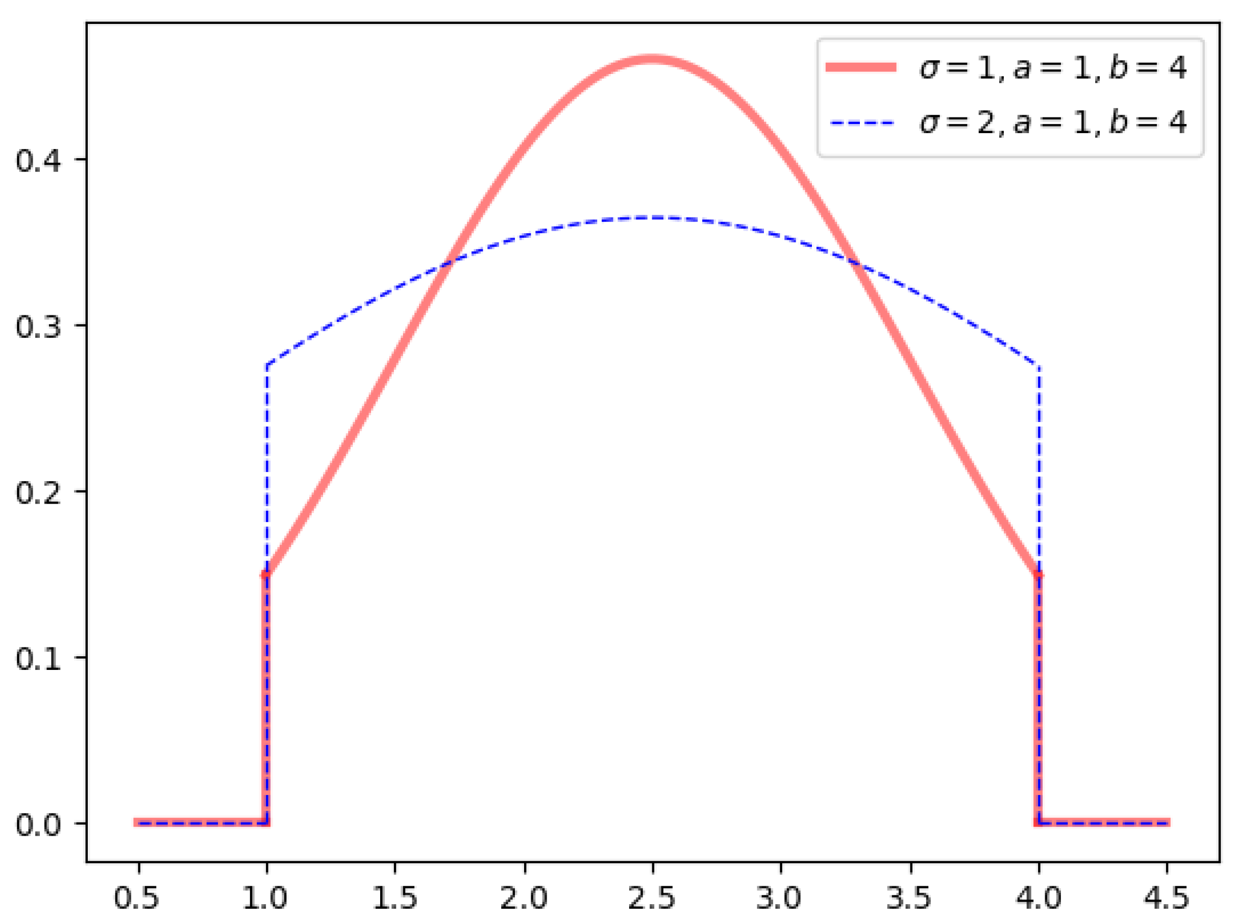
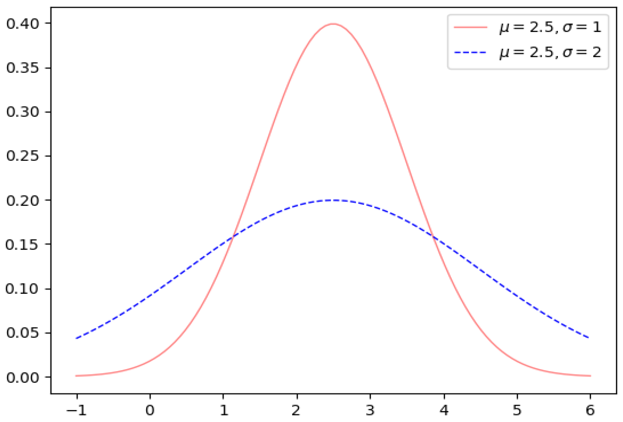
2.2. Intervals with Symmetric Truncated Normal Density Function

Definition 2 is mainly due to the authors of reference [24], and it has been applied in industry [25]. The normalization of probability on interval was verified independently after Definition 2.

Definition 2.

The symmetric truncated interval normal density function (short for truncated normal density) $f(x,a,b,\sigma )$is as formula (6)

$$f(x,a,b,\sigma )=\{\begin{array}{l}\frac{1}{\sigma }\cdot \frac{\varphi (\frac{x-\mu }{\sigma })}{\Phi (\frac{b-\mu }{\sigma })-\Phi (\frac{a-\mu }{\sigma })},a\le x\le b\\ 0,\hspace{1em}\hspace{1em}\hspace{1em}\hspace{1em}\hspace{1em}\hspace{1em}x<a \mathrm{or} x>b \end{array}$$

(6)

where$\mu =\frac{b+a}{2}$, the function curve is symmetric about$\mu =\frac{b+a}{2}$, that is,$\mu =\frac{b+a}{2}$is the axis of symmetry as shown in Figure 1;$a,b$respectively represent the upper and lower bounds of the interval$[a,b]$;$\varphi (x)$is the probability density function of the standard normal distribution;$\Phi (x)$is the standard normal cumulative distribution function;$\sigma$is the parameter for the shape of the interval normal density. In Figure 1, the larger$\sigma$corresponds to a flatter function curve, which is similar to meaning in the normal probability density. The following verification in formula (7) shows that the formula “${\displaystyle {\int }_a^{b}f(x,a,b,\sigma )}=1$” holds, which must be satisfied according to Definition 1.

$$\begin{array}{l}{\displaystyle {\int }_a^{b}f(x,a,b,\sigma )}\mathrm{d}x={\displaystyle {\int }_a^b\frac{1}{\sigma }\frac{\varphi (\frac{x-\mu }{\sigma })}{\Phi (\frac{b-\mu }{\sigma })-\Phi (\frac{a-\mu }{\sigma })}}\mathrm{d}x={\displaystyle {\int }_a^b\frac{\varphi (\frac{x-\mu }{\sigma })}{\Phi (\frac{b-\mu }{\sigma })-\Phi (\frac{a-\mu }{\sigma })}}\mathrm{d}(\frac{x-\mu }{\sigma })\\ \stackrel{\frac{x-\mu }{\sigma }=z}{=}\frac{{\displaystyle {\int }_{\frac{a-\mu }{\sigma }}^{\frac{b-\mu }{\sigma }}\varphi (z)\mathrm{dz}}}{\Phi (\frac{b-\mu }{\sigma })-\Phi (\frac{a-\mu }{\sigma })}=\frac{\Phi (\frac{b-\mu }{\sigma })-\Phi (\frac{a-\mu }{\sigma })}{\Phi (\frac{b-\mu }{\sigma })-\Phi (\frac{a-\mu }{\sigma })}=1\end{array}$$

(7)

Figure 1 shows the truncated normal density curve for $a=1,b=4,\sigma =1$, and $\sigma =2$. Figure 2 shows the function curve of the normal density function when $\mu =2.5,\sigma =1$, and $\sigma =2$.

As shown in Figure 1, when $x\notin [a,b]$ and $f(x,a,b,\sigma )\equiv 0$, which are different from the normal probability density function. Combining definitions 1 and 2, the definition of the interval normal interval can be given as follows:

Definition 3.

(Symmetric truncated normal interval, short for truncated normal interval) An interval random error X is a truncated normal interval, if X is in the range $[a, b]$,$a\le b$, and the probability density$f(x,a,b,\sigma )$of X has the form of formula (6). The truncated normal interval X can be denoted by${[a, b]}_{f_{\sigma }}$,$f(x,a,b,\sigma )$.

Obviously, taking $x=\frac{b+a}{2}$ as the midline, the errors variables appearing on the left and right sides of the midline are symmetrical. The normal truncation interval is used to represent uncertain parameters in the method introduced later in this paper.

Properties 1 and 2 (introduced in reference [26]) show how to calculate the expectation and variance of the truncated normal interval, respectively.

Property 1.

The expectation of truncated normal interval $X(X={[a, b]}_{f_{\sigma }},f(x,a,b,\sigma ))$is:

$$E(X)=(a+b)/2$$

(8)

Property 2.

The variance of truncated normal interval $X(X={[a, b]}_{f_{\sigma }},f(x,a,b,\sigma ))$is:

$$D(X)={\sigma }^2(1-\frac{\frac{b-a}{2\sigma }\varphi (\frac{b-a}{2\sigma })-\frac{a-b}{2\sigma }\varphi (\frac{a-b}{2\sigma })}{\Phi (\frac{b-a}{2\sigma })-\Phi (\frac{a-b}{2\sigma })})$$

(9)

The variance and expectation of the truncated normal interval were also independently verified by the following Maple2020 codes:

phi:= x -> exp(−1/2*x^2)/sqrt(2*Pi);

Phi:= x -> 1/2 + 1/2*erf(1/2*sqrt(2)*x);

f:= (x, a, b, sigma) -> phi((x − 1/2*a − 1/2*b)/sigma)/(sigma*(Phi((1/2*b − 1/2*a)/sigma) − Phi((1/2*a − 1/2*b)/sigma)));

E(X) = int(x*f(x, a, b, sigma), x = a .. b);

Var[1]:= X -> int(x^2*f(x, a, b, sigma), x = a .. b) − int(x*f(x, a, b, sigma), x = a .. b)^2;

Var[2]:= X -> sigma^2*(1 − ((1/2*b/sigma − 1/2*a/sigma)*phi(1/2*b/sigma − 1/2*a/sigma) − (1/2*a/sigma − 1/2*b/sigma)*phi(1/2*a/sigma − 1/2*b/sigma))/(Phi(1/2*b/sigma − 1/2*a/sigma) − Phi(1/2*a/sigma − 1/2*b/sigma)));

simplify(Var[1](X) − Var[2](X));

Lemma 1.

$X(X={[a, b]}_{f_{\sigma }},f(x,a,b,\sigma ))$is a truncated normal interval, which$f(x,a,b,\sigma )$is introduced in Definition 2. where$C_1$is the positive real number. Then,$Y(Y=C_{1}X)$must be a truncated normal interval with probability density$f(y,C_{1}a,C_{1}b,C_1\sigma )$in$[C_{1}a, C_{1}b]$.

Proof. 

According to probability knowledge, formula (10) can be obtained.

$$F_{Y\_cpf}(y)=P(Y\le y)=P(C_{1}X\le y)=P(X\le \frac{y}{C_1})=F_{X\_cpf}(\frac{y}{C_1})$$

(10)

In formula (10), $F_{X\_cpf}(x)$ and $F_{Y\_cpf}(y)$ are the cumulative distribution functions of X and Y, respectively. After calculating the derivative of y in Equation (10), the probability density of Y can be obtained as follows:

$$f_{Y\_pdf}(y)=f_{X\_pdf}(\frac{y}{C_1})\cdot \frac{1}{C_1}=f(\frac{y}{C_1},a,b,\sigma )\cdot \frac{1}{C_1}$$

(11)

In addition:

$$X={[a, b]}_{f_{\sigma }}\Rightarrow a\le X\le b\stackrel{C_1>0}{\Rightarrow }{C}_{1}a\le C_{1}X\le C_{1}b\Rightarrow C_{1}a\le Y\le C_{1}b$$

(12)

According to formula (6) and formula (11), we have:

$$\begin{gathered} f_{Y\_pdf}(y)=f(\frac{y}{C_1},a,b,\sigma )\cdot \frac{1}{C_1}=\{\begin{array}{l}\frac{1}{\sigma }\cdot \frac{\varphi (\frac{\frac{y}{C_1}-\mu }{\sigma })}{\Phi (\frac{b-\mu }{\sigma })-\Phi (\frac{a-\mu }{\sigma })}\cdot \frac{1}{C_1}, a\le \frac{y}{C_1}\le b\\ 0,\hspace{1em}\hspace{1em}\frac{y}{C_1}\le a , \mathrm{or}\frac{y}{C_1}\ge b\end{array}= \\ \{\begin{array}{l}\frac{1}{C_1\sigma }\cdot \frac{\varphi (\frac{\frac{y}{C_1}-\mu }{\sigma })}{\Phi (\frac{b-\mu }{\sigma })-\Phi (\frac{a-\mu }{\sigma })},C_{1}a\le y\le C_{1}b\\ 0,\hspace{1em}\hspace{1em}y\le C_{1}a , \mathrm{or} y\ge C_{1}b\end{array}=\{\begin{array}{l}\frac{1}{C_1\sigma }\cdot \frac{\varphi (\frac{y-C_1\mu }{C_1\sigma })}{\Phi (\frac{C_{1}b-C_1\mu }{C_1\sigma })-\Phi (\frac{C_{1}a-C_1\mu }{C_1\sigma })}, C_{1}a\le y\le C_{1}b\\ 0,\hspace{1em}\hspace{1em}y\le C_{1}a , \mathrm{or} y\ge C_{1}b\end{array} \end{gathered}$$

That is, formula (13) is obtained:

$$f_{Y\_pdf}(y)=\{\begin{array}{l}\frac{1}{C_1\sigma }\cdot \frac{\varphi (\frac{y-C_1\mu }{C_1\sigma })}{\Phi (\frac{C_{1}b-C_1\mu }{C_1\sigma })-\Phi (\frac{C_{1}a-C_1\mu }{C_1\sigma })}, C_{1}a\le y\le C_{1}b\\ 0,\hspace{1em}\hspace{1em}y\le C_{1}a , \mathrm{or} y\ge C_{1}b\end{array}$$

(13)

Formula (13) conforms to the definition of “truncated normal density” introduced in Definition 2. Thus, we have:

$$f_{Y\_pdf}(y)=\left\{\begin{array}{l}\frac{1}{C_1\sigma }\cdot \frac{\varphi (\frac{y-C_1\mu }{C_1\sigma })}{\Phi (\frac{C_{1}b-C_1\mu }{C_1\sigma })-\Phi (\frac{C_{1}a-C_1\mu }{C_1\sigma })}, C_{1}a\le y\le C_{1}b\\ 0,\hspace{1em}\hspace{1em}y\le C_{1}a , \mathrm{or} y\ge C_{1}b\end{array}\right\}=f(y,C_{1}a,C_{1}b,C_1\sigma )$$

(14)

In summary, according to the definitions of the truncated normal interval introduced in Definition 3, $Y(Y=C_{1}X)$ can be regarded as the truncated normal interval with $Y={[C_{1}a, C_{1}b]}_{f_{\sigma c_1}},f(y,C_{1}a,C_{1}b,C_1\sigma )$. □

Lemma 2.

$X(X={[a, b]}_{f_{\sigma }},f(x,a,b,\sigma ))$is a truncated normal interval, which$f(x,a,b,\sigma )$is introduced in Definition 2.$C_0$is a real constant. Then,$Y(Y=X+C_0)$must be a truncated normal interval with probability density$f(y,a+C_0, b+C_0,\sigma )$in$[a+C_0, b+C_0]$.

Proof. 

According to probability knowledge, we have:

$$F_{Y\_cpf}(y)=P(Y\le y)=P(X+C_0\le y)=P(X\le y-C_0)$$

(15)

After calculating the derivation of formula (15) on y, we have

$$\begin{array}{l}{f}_{Y\_pdf}(y)=f_{X\_pdf}(y-C_0)=f(y-C_0,a,b,\sigma )=\{\begin{array}{l}\frac{1}{\sigma }\cdot \frac{\varphi (\frac{y-C_0-\mu }{\sigma })}{\Phi (\frac{b-\mu }{\sigma })-\Phi (\frac{a-\mu }{\sigma })},\hspace{1em}a\le y-C_0\le b\\ 0,\hspace{1em}\hspace{1em}y-C_0<a , \mathrm{or} y-C_0>b \end{array}=\\ \left\{\begin{array}{l}\frac{1}{\sigma }\cdot \frac{\varphi (\frac{y-(C_0+\mu )}{\sigma })}{\Phi (\frac{b-\mu }{\sigma })-\Phi (\frac{a-\mu }{\sigma })},\hspace{1em}a+C_0\le y{\le }_{0}b+C_0\\ 0,\hspace{1em}y<a+C_0 ,\hspace{1em}\mathrm{or} y>b+C_0 \end{array}\right\}=f(y,a+C_0, b+C_0,\sigma )\end{array}$$

Because $\mu =\frac{a+b}{2}$, we have $C_0+\mu =\frac{(a+C_0)+(b+C_0)}{2}$.

In summary, $Y(Y=X+C_0)$ can be treated as a truncated normal interval with ${[a+C_0, b+C_0]}_{f{\sigma }_{}}$ and $f(y,a+C_0, b+C_0,\sigma )$. □

Theorem 1.

$X(X={[a, b]}_{f_{\sigma }},f(x,a,b,\sigma ))$is a truncated normal interval,$C_0,C_1$are two real constants, and$C_1>0$, and$Y(Y=C_{1}X+C_0)$is also a truncated normal interval with the probability density$f(y,C_{1}a+C_0, C_{1}b+C_0,C_1\sigma )$on the interval$[C_{1}a+C_0, C_{1}b+C_0]$.

Proof. 

According to Lemma 1, $C_{1}X$ is a truncated normal interval with probability density $f(y,C_{1}a,C_{1}b,C_1\sigma )$ on the interval, $[C_{1}a, C_{1}b]$ and from Lemma 2, $Y(Y=C_{1}X+C_0)$ is also a truncated normal interval on the interval $[C_{1}a+C_0, C_{1}b+C_0]$ with probability density $f(y,C_{1}a+C_0,C_{1}b+C_0,C_1\sigma )$. □

The parameter $\sigma$ of the truncated normal interval $X(X={[a, b]}_f,f(x,a,b,\sigma ))$ is not the standard deviation of $X$. $X$ can be regarded as a random variable generated by the normal random variable $Y\sim N(\frac{a+b}{2},{\sigma }^2)$ by truncating $Y$ on [a, b]. As introduced in properties 1 and 2, the expectation of $X$ can be calculated by a and b, and the variance of $X$ is calculated by a, b, and $\sigma$. According to Theorem 1, the operations of truncated normal intervals introduced in Section 2.1, can be partially accelerated, especially for operations on truncated normal intervals. The following section introduces the reasoning methods based on truncated normal intervals.

3. Truncated Normal Interval-Based Reasoning Method

According to Definition 3, truncated normal intervals can be regarded as an extension of the interval by adding a truncated normal density to the interval. Hence, this makes the interval-based polynomial reasoning method (such as the methods from reference [20,21,22]) still valid for truncated normal intervals. In Section 3.2, we improved the reasoning methods [20,21] by adding the calculation of the truncated normal density into them. Before that, we introduce an implication relationship.

3.1. Reasoning Method between Polynomial Errors Assertions

3.1.1. Implication Relationship

In this section, we first introduce the polynomial error assertion, its zero set, Axiom 1, and the implication relationship, which were proposed by reference [22]. The implication relationship between assertions is the fundamental rule in the reasoning method based on theorem proving. The equivalence relationship can be attributed to assessing whether there are implication relationships with each other [27]. Hence, only the implication relationship is discussed below.

Definition 4 (Polynomial error assertion, PEA).

$\overline{\phi }$is a PEA if$\overline{\phi }$and$\overline{f_1},\overline{f_2},\dots ,\overline{f_k}$satisfy (16) and (17), respectively.

$$\overline{\phi }=\{\begin{array}{l}\overline{f_1}(x_1,\dots ,x_n)=0\\ \overline{f_2}(x_1,\dots ,x_n)=0\\ \dots \\ \overline{f_k}(x_1,\dots ,x_n)=0\end{array}$$

(16)

$$\overline{f_i}(x_1,\dots ,x_n)={\displaystyle \sum _{j=0\dots m}\overline{c_{ij}}{x}_1^{{\alpha }_{ij1}}{x}_2^{{\alpha }_{ij2}}\dots \dots x_n^{{\alpha }_{ijn}}}{,}^{} i=1,2\dots \dots k, \overline{c_j}=[c_j^{-},c_j^{+}], j=0,\dots m$$

(17)

Definition 5 (Real zero set of PEAs, short for zero set of PEAs).

$\overline{\phi }$is a PEA. The real zero set of$\overline{\phi }$, denoted by$zero(\overline{\phi })$, satisfies (18).

$$zero(\overline{\phi })=zero(\overline{f_1})\cap zero(\overline{f_2})\cap \dots \dots \cap zero(\overline{f_n})$$

(18)

In addition,$zero(\overline{f_1}),zero(\overline{f_2}),\dots ,zero(\overline{f_n})$satisfies Formula (19).

$$zero(\overline{f_i})=\{(x_1,\dots ,x_n)|\forall c_{ij}\in \overline{c_{ij}}, and{\displaystyle \sum _{j=0\dots m_i}{c}_{ij}{x}_1^{{\alpha }_{ij1}}{x}_2^{{\alpha }_{ij2}}\dots \dots x_n^{{\alpha }_{ijn}}}=0,and (x_1,\dots ,x_n)\in {ℝ}^n\}$$

(19)

Apparently, the definition of the zero set of PEAs is self-consistent with that of classic polynomials. This is because when the upper and lower bounds of the interval are equal, the interval degenerates into a real number. For example, $[{\epsilon }^{-}, {\epsilon }^{+}]$ degenerates into a real number $\epsilon$ when $\epsilon ={\epsilon }^{-}={\epsilon }^{+}$. Here, the definition of the zero set of PEAs and that of the classical polynomial equations are identical.

Axiom 1.

${\overline{\phi }}_1$implies${\overline{\phi }}_2$(denoted as${\overline{\phi }}_1|={\overline{\phi }}_2$)$iff Zero({\overline{\phi }}_1)\subseteq Zero({\overline{\phi }}_2)$, where${\overline{\phi }}_1$and${\overline{\phi }}_2$are polynomials or PEAs.

For polynomials, here is an example of Axiom 1. Let. ${\phi }_1:x-5=0{,}^{}{\phi }_2:x^2-4x-5=0$. Now, we need to determine whether ${\phi }_1|={\phi }_2$, which means whether ${\phi }_1$ implies ${\phi }_2$. Simply put, if ${\phi }_1$ is true, then ${\phi }_2$ must be true. Indeed, $Zero({\phi }_1)\subseteq Zero({\phi }_2)$ must hold owing to $\left\{5\right\}\subseteq \{-1, 5\}$.

For PEAs, $Zero(\overline{\phi })$ is the set of all possible states of the system caused by the error parameters. In the polynomial-described system, the state of the system needs to satisfy specific polynomial equations, whose solutions define the safe area of the system in this state. For example, if the set $Zero(\overline{\phi })$ indicates the safe area in a certain state of the system, we find that the variable value x of the system in this state is not included in $Zero(\overline{\phi })$, which means that the system is unsafe at the moment, and the fault should be eliminated immediately.

3.1.2. Problems of Previous Reasoning Methods

For error polynomial assertions, the previous reasoning methods [20,21,22] are all based on only characterizing errors as intervals, while ignoring the probability distribution information of the errors within the interval. In fact, the probability information of errors in the interval does exist and can be obtained from the statistics of the previous data. For example, in a large number of statistics on the measurement results of a certain physical quantity by a certain sensor, it can always be obtained that the measurement values closer to the true value will appear more frequently than the measurement values farther away. Ignoring the probability information of errors may lead to incomplete reasoning results, which affects the validity of the reasoning methods.

The set $Zero(\overline{\phi })$ of all possible states caused by error parameters can be obtained. When designing the system, the impact of errors on the system should be fully considered. Thus, the system must have the ability to withstand the influence of errors. Hence, the system must allow the system states to appear at any position inside the set $Zero(\overline{\phi })$; that is, set $Zero(\overline{\phi })$ must be the subset of the designed state range of the system. Based on previous reasoning methods [20,21,22], if it is found that the state of the system ($x=(x_1,x_2,\dots ,x_n)$) at a certain time is not in the set $Zero(\overline{\phi })$, that is, $(x_1,x_2,\dots ,x_n)\in Zero(\overline{\phi })$ does not hold, then it indicates that there must be non-error factors (the non-error factors here and below are not the factors caused by similar uncertain parameters but the mechanical, electrical, and other factors that affect the performance of the system) affecting the system at this time, and the detection should be carried out immediately. In other words, only when we find that the system state is not in the set $Zero(\overline{\phi })$ can we conclude that there must be the influence of non-error factors by previous reasoning methods. The following question is: Can it be concluded in advance that there is a great possibility of non-error factors in the system when the system state is still inside set $Zero(\overline{\phi })$? Yes, but this requires more information about the error besides the interval. The focus of this study is to obtain such answers by combining statistical methods and reasoning methods.

3.2. Reasoning Method Based on Truncated Normal Interval

In this section, by introducing a truncated normal interval and combining the knowledge of probability and statistics, we generalize the methods in reference [20,21]. According to the quantile theory in statistics [28,29], the system state regions with a low probability in $Zero(\overline{\phi })$ can be marked. If the system states often appear in the low probability area within a certain time period, then there is reason to believe that there are non-error factors affecting the system at this time. Although, at this time, the non-error factors can be withstood by the system; however, for safety-critical systems, it is necessary to eliminate potential mechanical or electrical problems early. The specific steps of the reasoning method are given below, which can be applied to the linear error assertion and the nonlinear problem in which the cross section (cross plane) of $Zero(\overline{\phi })$ is a convex set, such as the example in Section 4.

In the following steps of the reasoning method, $x(t)$ is the observation vector of the system state variables $x_{1,}{x}_{2,}\dots ,x_n$ at time t: The error assertion that the system satisfies in a certain state is $\overline{\phi }$. Now, it is necessary to assess whether the system has non-error factors affecting the system at this time. The specific steps of the reasoning methods based on truncated normal intervals are given below.

Step 1: Calculate all the vertices of the set, $Zero(\overline{\phi })$ $v_1,v_2,\dots ,v_{2^n}$, and generate inequalities that represent the area $Zero(\overline{\phi })$.

Step 2: Put any internal point p of set $Zero(\overline{\phi })$ into the inequalities obtained in step 1 to obtain a specific inequality relationship.

Step 3: Put $x(t)$ into the inequalities obtained in step (2). If $x(t)$ cannot satisfy the inequalities, there must be non-error factors affecting the system. Here, fault detection is instantly required. If $x(t)$ satisfies the inequalities, proceed to step (4).

Step 4: Calculate the probability distribution information of the area represented by set $Zero(\overline{\phi })$, and calculate the set $\Omega$ ($\Omega$ is the subset of $Zero(\overline{\phi })$, $\Omega$ where represents the area where the system state $x(t)$ has a higher probability of occurrence when the system is running without potential failures). When $x(t)\notin \Omega$, it is still very likely that there are non-error factors in the system, and it is still necessary to detect the system to avoid non-error factors beyond the acceptable range of the system.

In the next section, an example is provided regarding the application of the reasoning method to the two-body problem of decentralized power systems under train acceleration.

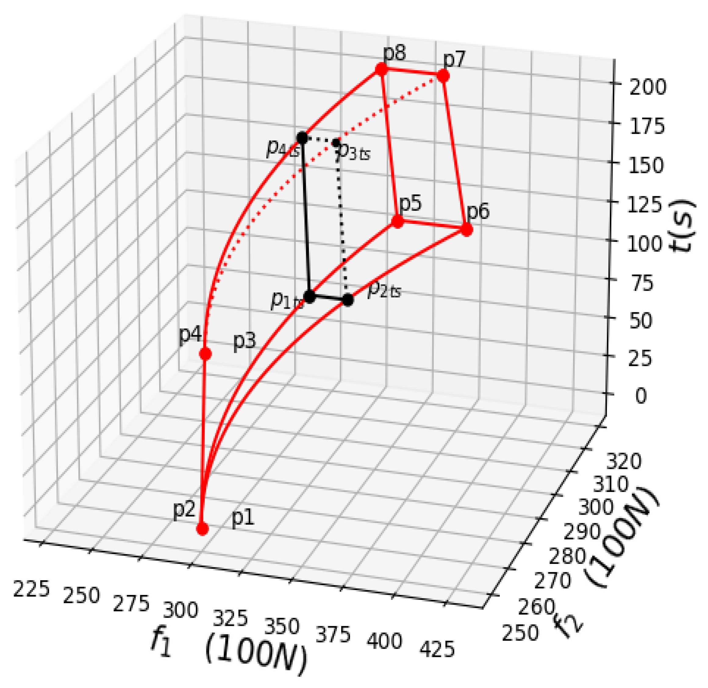
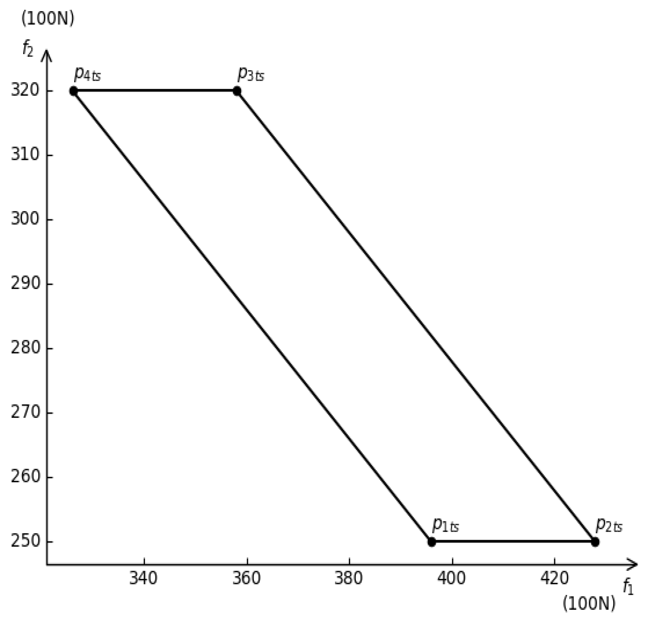
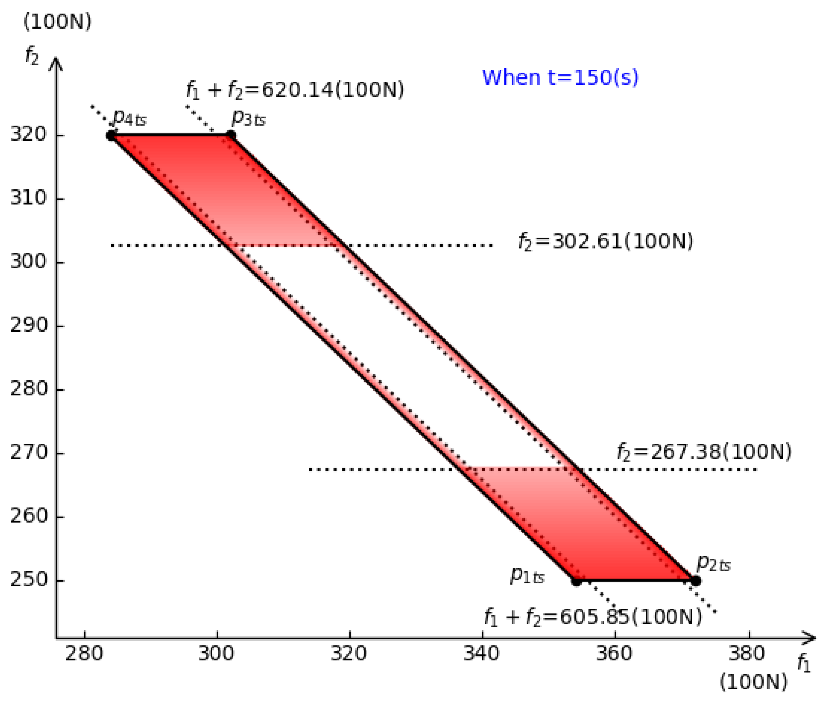
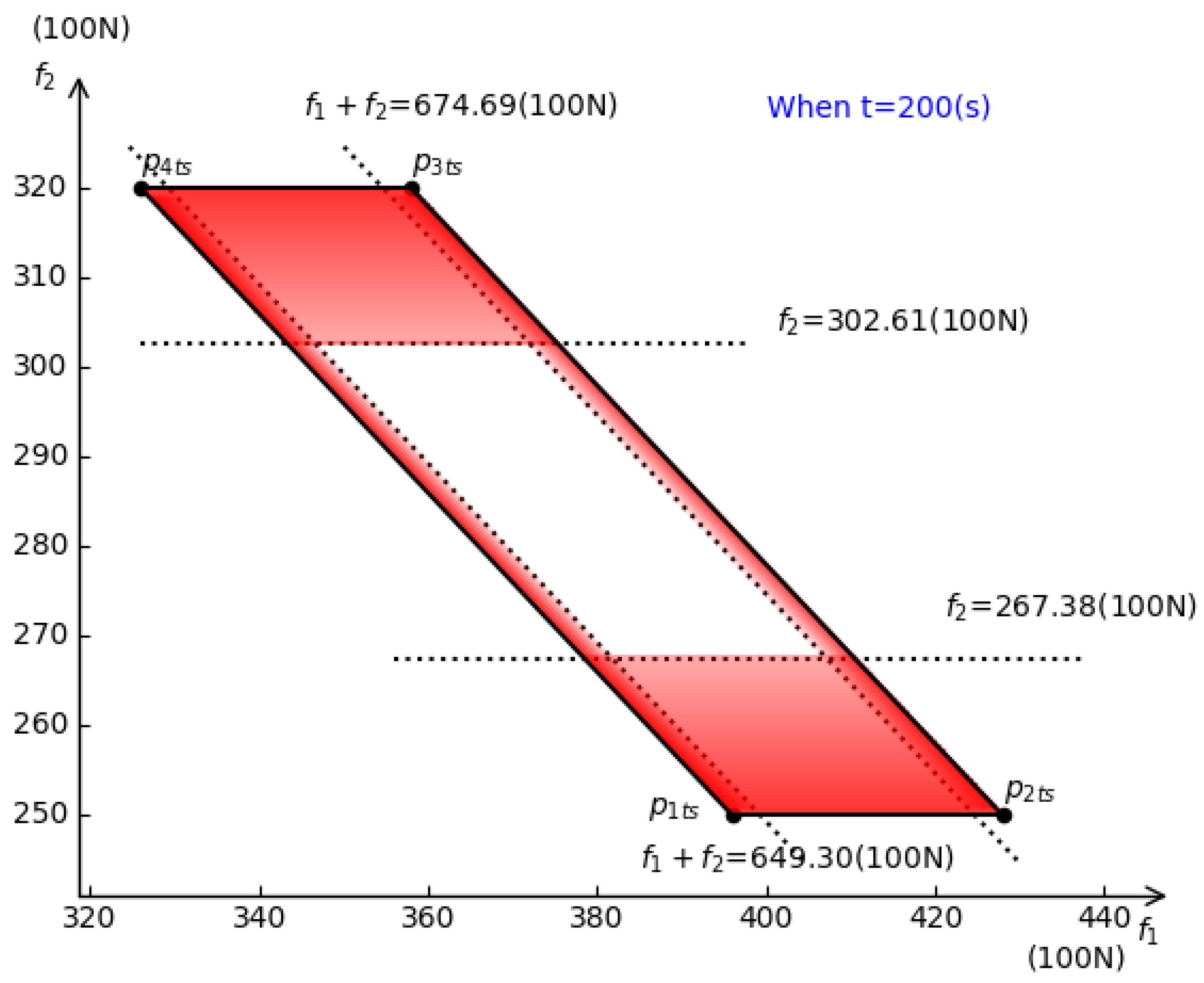
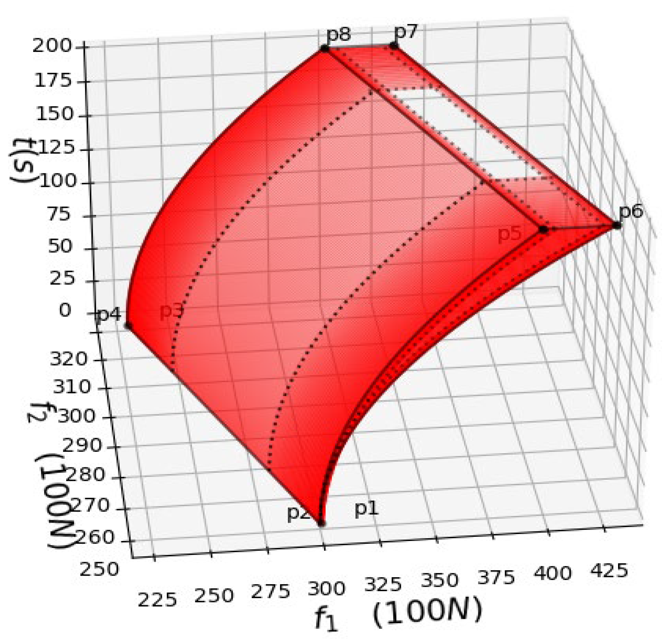
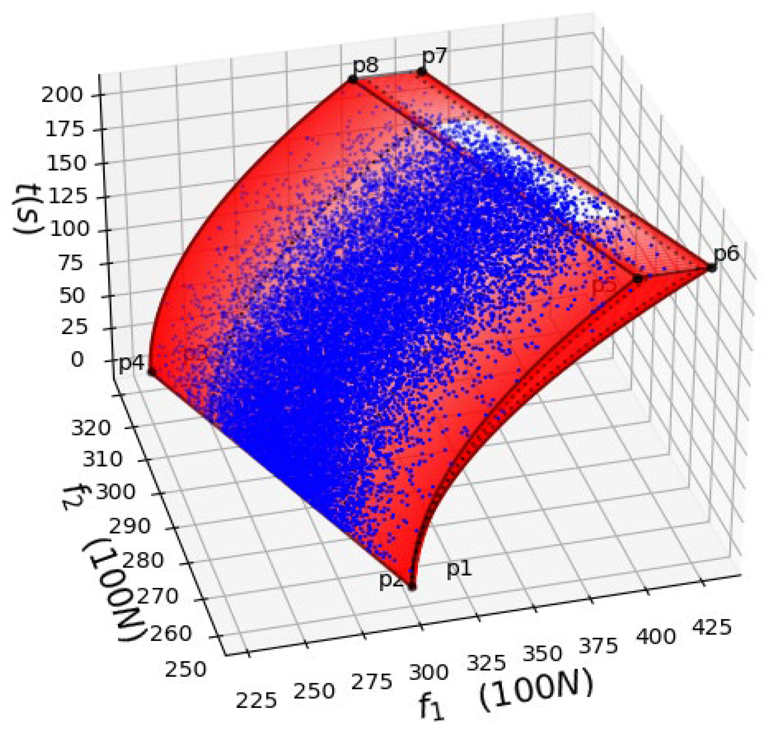
4. Verification of Two-Body Decentralized Power System during Train Acceleration

In Section 4.1, we present a case of the train acceleration state. In Section 4.2, we simulated the results obtained in Section 4.1, with a large number of random test cases.

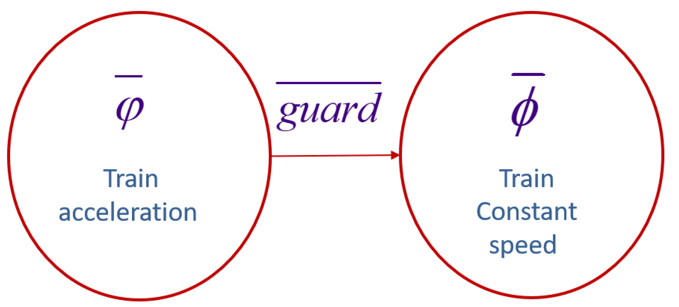
4.1. Two-Body Problem of Train Acceleration

Assume that the train has two carriages (the 8-carriage and 16-carriage problems can be obtained recursively from the two-carriage problem). The two carriages have independent power outputs. When the train starts, the train moves from the acceleration state to the constant-speed state. The guard (guard: $v=80 \mathrm{m}/\mathrm{s}=288 \mathrm{k}\mathrm{m}/\mathrm{h}$) is the transition condition from acceleration to a constant state, as shown in Figure 3. $\overline{\phi }$ and $\overline{\varphi }$ are the formulas that need to be satisfied in the acceleration state and the constant speed state, respectively. For example, in the acceleration state, if $\overline{\phi }$ is not satisfied, the train power output system runs abnormally. Here, immediate detection is required.

When the train is accelerating and starting, the mass sum (including passengers) of carriage 1 and carriage 2 is a fixed value M. During a certain acceleration of the train, there is a random flow of passengers between the two carriages. However, the total mass of the two carriages was constant. However, for passengers to experience a comfortable train ride, a constant acceleration ($a=4 \mathrm{m}/{\mathrm{s}}^{-2}$ in this case) must be maintained during the acceleration state. The power control system of the train has a complex feedback mechanism that can maintain stable acceleration during acceleration. However, whether there are potential mechanical or electrical faults requires further verification and analysis.

After 200 s of acceleration with $a=4 \mathrm{m}/{\mathrm{s}}^{-2}$, the train speed reached $v=288 \mathrm{km}/\mathrm{h}$. In the acceleration state with $a=4 \mathrm{m}/{\mathrm{s}}^{-2}$, some of the following parameters affect the power output: $M_1$ and $M_2$ represent the masses of two train cars (including passengers and their luggage), respectively; and $f_1,f_2$ represent the traction provided by carriage 1 and carriage 2, respectively, $f_{12}$ is the force of carriage 1 on carriage 2, $\zeta$ is a parameter related to air density and pressure, $a$ represents acceleration ($a=4 \mathrm{m}/{\mathrm{s}}^{-2}$), and g is the gravity acceleration ($g={10}_{} \mathrm{m}·{\mathrm{s}}^{-2}$). In a certain acceleration state, the sum of the masses of the two carriages is a fixed value of 110,000 kg. According to statistics of past passenger flow information and weather information during the same period, some of the above parameters can be regarded as truncated normal intervals, which were introduced in Section 2.2; that is, $M_1=m_1+\Delta m_1={[50,000,60,000]}_{h_1},h_1(x,50,000,60,000,{\sigma }_1)$; $M_2=m_2+\Delta m_2={[50,000,60,000]}_{h_2},h_2(x,50,000,60,000,{\sigma }_2)$; $\zeta ={[1.5,2]}_{h_{\zeta }}, h_{\zeta }(x,1.5,2,{\sigma }_{\zeta })$; $f_{12}={[0,2000]}_{h_{f12}}, h_{\zeta }(x,0,2000,{\sigma }_{f12})$. According to the knowledge of mechanics, we can obtain Equation (20):

$$\overline{\phi }=\{\begin{array}{l}{f}_1+f_2=\mathrm{M}g\mu +\mathrm{M}a+\zeta a^2{t}^2\\ f_2=M_{2}g\mu +M_{2}a+f_{12}\\ \mathrm{M}=M_1+M_2=110,000\\ M_1=m_1+\Delta m_1={[50,000, 60,000]}_{h_1}, h_1(x,50,000, 60,000,{\sigma }_1)\\ \zeta ={[1.5, 2]}_{h_{\zeta }}, h_{\zeta }(x,1.5, 2,{\sigma }_{\zeta })\\ f_{12}{=[0, 2000]}_{h_{f12}} , h_{f_{12}}(x,0, 2000, {\sigma }_{12})\end{array}$$

(20)

From the “step 1–step2” given in Section 3.2, the space area can be obtained shown in Figure 4 (The area surrounded by red lines, which short for red area as below).

The vertexes of $Zero(\overline{\phi })$ is shown in formula (21).

$$\{\begin{array}{l}{p}_{1t}=(30,000+0.24t^2,25,000)\\ p_{2t}=(30,000+0.32t^2,25,000)\\ p_{3t}=(23,000+0.32t^2,32,000)\\ p_{4t}=(23,000+0.24t^2,32,000)\end{array}$$

(21)

The possible power value at a certain time ${\mathrm{t}}_s$ (${\mathrm{t}}_s\in [0, 200]$) is the inside enclosed area (including the boundary) by the black line shown in Figure 5, which is short for the black area as shown below. The black area (it is a quadrilateral, as shown in Figure 6) is actually the horizontal section of the red area at $t={\mathrm{t}}_s$.

According to the definitions of the truncated normal interval and the arithmetic rules in Section 2.1 and Section 2.2, the probability distribution information of $f_1,f_2$ can be obtained.

The values of $f_1, f_2$ are determined using the other variables ($M_1,M_2,\zeta ,f_{12}$). First, the probability density of is calculated as $f_2$. Let $X=M_2(g\mu +a)$. According to Theorem 1, the probability density of $X$ can be obtained as $h_X\left(x)=h_2\right(x , 25000 , 32,000 ,0.5{\sigma }_2)$ From the second sub-formula ($f_2=M_{2}g\mu +M_{2}a+f_{12}$) in formula (20), and combined with the arithmetic rules of the truncated normal interval introduced in Section 2.1, the probability density of $f_2$ can be obtained as formula (22):

$$\{\begin{array}{l}h\left(f_2\right)\stackrel{X=M_2(\mathrm{g}\mu +\mathrm{a})}{=}{\displaystyle {\int }_0^{2000}{h}_X(f_2-f_{12})\cdot h_{f_{12}}(f_{12},0,2000,{\sigma }_{12})}\mathrm{d}(f_{12})\hspace{1em}25,000\le f_2\le 32,000\\ h(f_2)=0 \hspace{1em}\hspace{1em}\hspace{1em}\hspace{1em}\hspace{1em}\hspace{1em}\hspace{1em}\hspace{1em}\hspace{1em}\hspace{1em}\hspace{1em}\hspace{1em}\hspace{1em}\hspace{1em}\hspace{1em}\hspace{1em}\hspace{1em}\hspace{1em}\hspace{1em}\hspace{1em}\hspace{1em}{f}_2<25,000 \mathrm{or} f_2>32,000\end{array}$$

(22)

After calculating Equation (22), $h\left(f_2\right)$ (when $25,000\le f_2\le 32,000$) can be obtained as formula (23):

$$h\left(f_2\right)=\frac{-\left(\sqrt{2}{e}^{-\frac{2\left(f_2^2-57,000f_2+812,250,000\right)}{{\sigma }_2^2+4{\sigma }_{12}^2}}\left(-\mathrm{erf}\left(\frac{2\left({\sigma }_{12}^2{f}_2+250{\sigma }_2^2-27,500{\sigma }_{12}^2\right)\sqrt{2}}{{\sigma }_{12}^2{\sigma }_2^2\sqrt{\frac{{\sigma }_2^2+4{\sigma }_{12}^2}{{\sigma }_{12}^2{\sigma }_2^2}}}\right)+\mathrm{erf}\left(\frac{2\sqrt{2}\left({\sigma }_{12}^2{f}_2-250{\sigma }_2^2-29,500{\sigma }_{12}^2\right)}{{\sigma }_{12}^2{\sigma }_2^2\sqrt{\frac{{\sigma }_2^2+4{\sigma }_{12}^2}{{\sigma }_{12}^2{\sigma }_2^2}}}\right)\right)\right)}{2\sqrt{\pi }{\sigma }_2{\sigma }_{12}\sqrt{\frac{{\sigma }_2^2+4{\sigma }_{12}^2}{{\sigma }_{12}^2{\sigma }_2^2}}\cdot \mathrm{erf}\left(\frac{2500\sqrt{2}}{{\sigma }_2}\right)\cdot \mathrm{erf}\left(\frac{500\sqrt{2}}{{\sigma }_{12}}\right)}$$

(23)

The function $\mathrm{erf}\left(x\right)$ appearing in formula (23) is $\mathrm{erf}\left(x\right)=\frac{2}{\sqrt{\pi }}{\displaystyle {\int }_0^x{{\displaystyle e}}^{{{\displaystyle -t}}^2}dt}$.

In contrast, let $Z$ be the sum of $f_1$ and $f_2$, that is, $Z=f_1+f_2$. From the first sub-formula ($f_1+f_2=\mathrm{M}g\mu +\mathrm{M}a+\zeta a^2{t}^2$) in formula (20), when $t>0$, the probability density of $Z=f_1+f_2$ can be obtained as formula (24):

$$h_{f_1+f_2}(Z=f_1+f_2)=\{\begin{array}{l}{h}_{\zeta }(z,1.5a^2{t}^2+\mathrm{M}(g\mu +a),2a^2{t}^2+\mathrm{M}(g\mu +a),a^2{t}^2{\sigma }_{\zeta }) 0.24t^2+55,000\le z\le 0.32t^2+55,000\\ 0\hspace{1em}\hspace{1em}\hspace{1em}\hspace{1em}\hspace{1em}\hspace{1em}\hspace{1em}\hspace{1em}\hspace{1em}\hspace{1em}\hspace{1em}\hspace{1em}\hspace{1em}\hspace{1em}\hspace{1em}\hspace{1em}\hspace{1em}\hspace{1em}\hspace{1em}z<0.24t^2+55,000 ,\mathrm{or} z>0.32t^2+55,000 \end{array}$$

(24)

After calculating formula (24), $h_{f_1+f_2}(Z=f_1+f_2)$ (when $0.24t^2+55,000\le z\le 0.32t^2+55,000, \mathrm{and} t>0$) can be obtained as Equation (25):

$$h_{f_1+f_2}(Z=f_1+f_2)=h_{\zeta }(z,0.24t^2+55,000,0.32t^2+55,000,0.16t^2{\sigma }_{\zeta })=\frac{25\sqrt{2}{e}^{\frac{-625{\left(z-\frac{7t^2}{25}-55,000\right)}^2}{32t^4{\sigma }_{\zeta }^2}}}{8t^2{\sigma }_{\zeta }\sqrt{\pi }\cdot \mathrm{erf}\left(\frac{\sqrt{2}}{8{\sigma }_{\zeta }}\right)}$$

(25)

When $z<0.24t^2+55,000$ or $z>0.32t^2+55,000$, $h(Z=f_1+f_2)=0$; When $t=0$ and $0.24t^2+55,000\le z\le 0.32t^2+55,000$, $h(Z=f_1+f_2)=\delta (x)$. $\delta \left(x\right)$ is the Dirac δ function.

The codes of Maple2020 to obtain the results of Equations (23) and (25) are as follows:

phi:= x -> exp(−1/2*x^2)/sqrt(2*Pi);

Phi:= x -> 1/2 + 1/2*erf(1/2*sqrt(2)*x);

f:= (x, a, b, sigma) -> phi((x − 1/2*a − 1/2*b)/sigma)/(sigma*(Phi((1/2*b − 1/2*a)/sigma) − Phi((1/2*a − 1/2*b)/sigma)));

h(f[2], sigma[12], sigma[2]):= int(f(f[2] − f[12], 25,000, 30,000, 1/2*sigma[2])*f(f[12], 0, 2000, sigma[12]), f[12] = 0 .. 2000);

f(z, 6/25*t^2 + 55,000, 8/25*t^2 + 55,000, 4/25*t^2*sigma[Zeta]);

According to the analysis of historical data of train operations in the past, ${\sigma }_2,{\sigma }_{12}$ and ${\sigma }_{\zeta }$ can be obtained by parameter estimation methods. The following shows the division of $Zero(\overline{\phi })$ when ${\sigma }_{\zeta }=0.15,{\sigma }_2=2000,{\sigma }_{12}=400$ and quantile $\alpha =0.1$. The values of the upper and lower quantiles were calculated using the relevant integral equation. The lower quantile of $f_2$ is calculated using Equation (26).

$${\displaystyle {\int }_{25,000}^{f_2}h(f_2)\mathrm{d}}\left(f_2\right)=\alpha /2=0.05\Rightarrow {\left(f_2\right)}_1\approx 26,738\left(\mathrm{N}\right)$$

(26)

The upper quantile of $f_2$ is calculated as formula (27).

$${\displaystyle {\int }_{f_2}^{32,000}h(f_2)\mathrm{d}}\left(f_2\right)=\alpha /2=0.05\Rightarrow {\left(f_2\right)}_2\approx 30,261\left(\mathrm{N}\right)$$

(27)

The lower quantile of $Z=f_1+f_2$ is calculated as formula (28).

$${\displaystyle {\int }_{\frac{6\cdot t^2}{25}+55,000}^z{h}_{f_1+f_2}(z)\mathrm{d}z}=0.05\Rightarrow z_1=\frac{35\sqrt{2}{t}^2-6\cdot \mathrm{Root}\_\mathrm{Of}\left(10\cdot \mathrm{erf}(Z)-9\cdot \mathrm{erf}(\frac{5\sqrt{2}}{6})\right)\cdot t^2+6,875,000\sqrt{2})\sqrt{2}}{250}$$

(28)

In Equation (28), $\mathrm{Root}\_\mathrm{Of}\left(10\cdot \mathrm{erf}(Z)-9\cdot \mathrm{erf}(\frac{5\sqrt{2}}{6})\right)$ represents the root of equation $10\cdot \mathrm{erf}(Z)-9\cdot \mathrm{erf}(\frac{5\sqrt{2}}{6})=0$. Similarly, the upper quantile of $Z=f_1+f_2$ is calculated using Equation (29).

$${\displaystyle {\int }_z^{\frac{8\cdot t^2}{25}+55,000}{h}_{f_1+f_2}(z)\mathrm{d}z}=0.05\Rightarrow z_2=\frac{35\sqrt{2}{t}^2-6\cdot \mathrm{Root}\_\mathrm{Of}\left(10\cdot \mathrm{erf}(Z)+9\cdot \mathrm{erf}(\frac{5\sqrt{2}}{6})\right)\cdot t^2+6,875,000\sqrt{2})\sqrt{2}}{250}$$

(29)

According to the numerical calculation from formulas (28) and (29), when t = 150(s), $z_1\approx 60,585\left(\mathrm{N}\right), z_2=62,014\left(\mathrm{N}\right)$; when t = 200(s), $z_1\approx 64930\left(\mathrm{N}\right), z_2=67469\left(\mathrm{N}\right)$.

Figure 7 and Figure 8 show the division of $Zero(\overline{\phi })$ by the quantiles (these quantiles are obtained by formulas (26)–(29)) when t = 150 s and t = 200 s, respectively.

Constant acceleration ($a=4 \mathrm{m}/{\mathrm{s}}^{-2}$) ensures the stability of the train and the good riding experience of the passengers. During the acceleration of the train, the error parameters are uncertain, which leads to a real-time adjustment of the power output of the train. When the truncated normal intervals are given as $M_1={[50,000,60,000]}_{h_1}$,$\zeta ={[1.5, 2]}_{h_{\zeta }}$, and $f_{12}=[0,2000{]}_{h_{f12}}$, the red areas in Figure 7 and Figure 8 represent the areas with low probability of occurrence of train power output $f_1,f_2$, and the red transparency (transparency is the concept of alpha blending about color) in the red area is proportional to the probability of $f_1,f_2$. Hence, the higher the red transparency, the higher the probability of $f_1,f_2$ in the red areas of Figure 7 and Figure 8. In other words, during the acceleration of the train (t = [0,200]), if the values of $f_1$ and $f_2$ appear in the red area for a period of time, it is reasonable to believe that there are non-error factors in the power system at this time, and the system must be checked for safety in time to inspect whether there are mechanical or electrical faults. The parallelogram in Figure 8 (the area enclosed by $P_{1t}{P}_{2t}{P}_{3t}{P}_{4t}$) is all possible areas of system power distribution caused by error parameters when t = 200. When designing the system, it is necessary to fully estimate the possible errors, and the power range $f_1,f_2$ must cover the $P_{1t}{P}_{2t}{P}_{3t}{P}_{4t}$ area to ensure that the system has the ability to withstand the error parameters. As time passes, the mechanical equipment of the trains will inevitably wear out. Hence, it is necessary to detect factors that may cause system failure in time. This section discusses how to divide the $P_{1t}{P}_{2t}{P}_{3t}{P}_{4t}$ area according to statistical knowledge. This is helpful for the safe operation of the system. Figure 9 shows the division of Figure 4, when $\alpha =0.1$ and $t=\left(0,200\right]$.

From (26)–(29), we obtain inequality(30) below, which represents the white area in Figure 9.

$$\{\begin{array}{l}\frac{35\sqrt{2}{t}^2-6\cdot \mathrm{Root}\_\mathrm{Of}\left(10\cdot \mathrm{erf}(Z)-9\cdot \mathrm{erf}(\frac{5\sqrt{2}}{6})\right)\cdot t^2+6,875,000\sqrt{2})\sqrt{2}}{250}\le f_1+f_2\le \frac{35\sqrt{2}{t}^2-6\cdot \mathrm{Root}\_\mathrm{Of}\left(10\cdot \mathrm{erf}(Z)+9\cdot \mathrm{erf}(\frac{5\sqrt{2}}{6})\right)\cdot t^2+6,875,000\sqrt{2})\sqrt{2}}{250}\\ 26,738\le f_2\le 30,216\end{array}$$

(30)

The red area in Figure 9 indicates a low occurrence probability of $f_1,f_2$. It is unlikely that $f_1$ and $f_2$ will be in the red area for a long time, which means that there is a high possibility of non-error factors. Although the system can withstand it sometimes, early detection is still necessary for safety-critical systems.

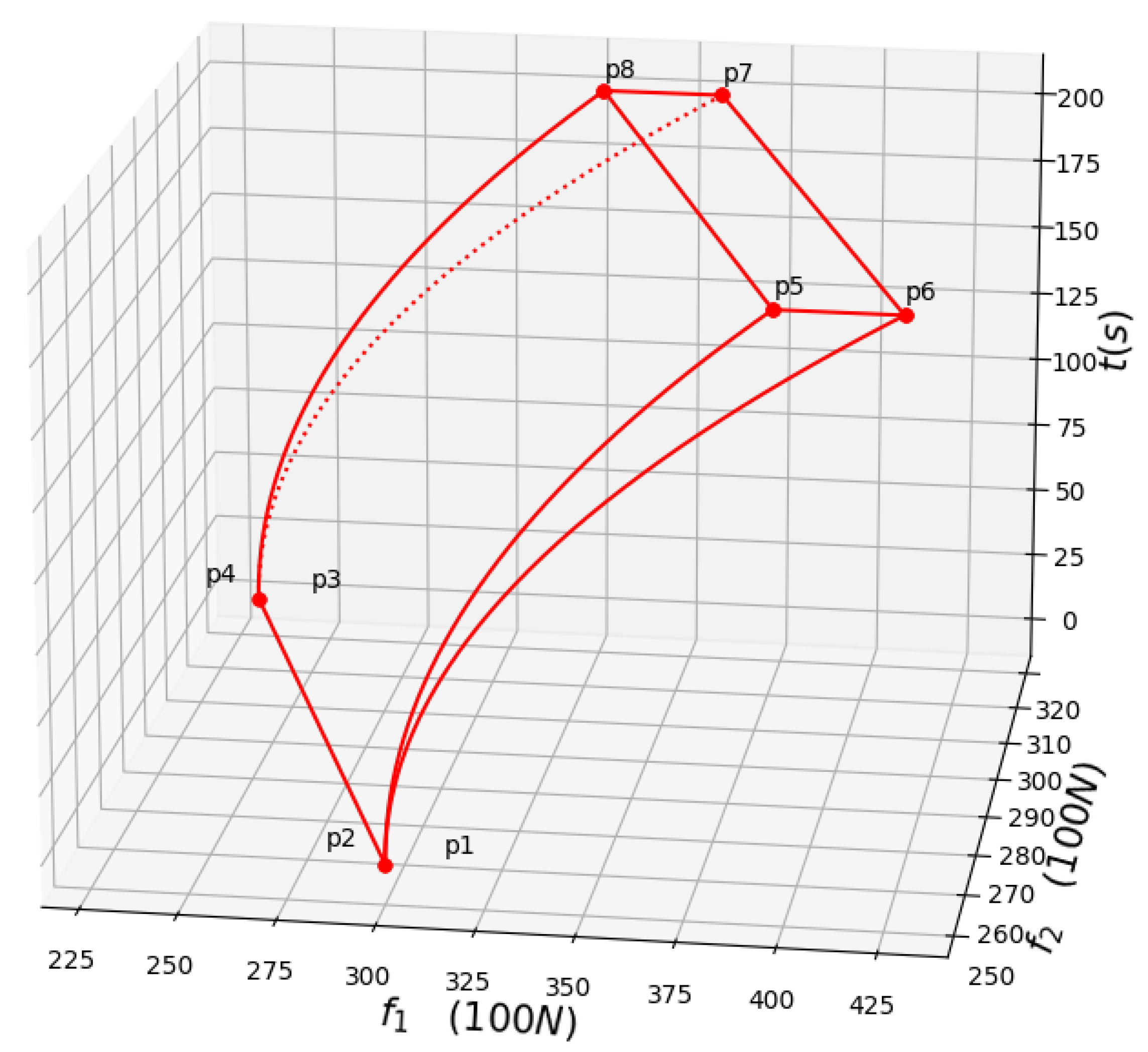
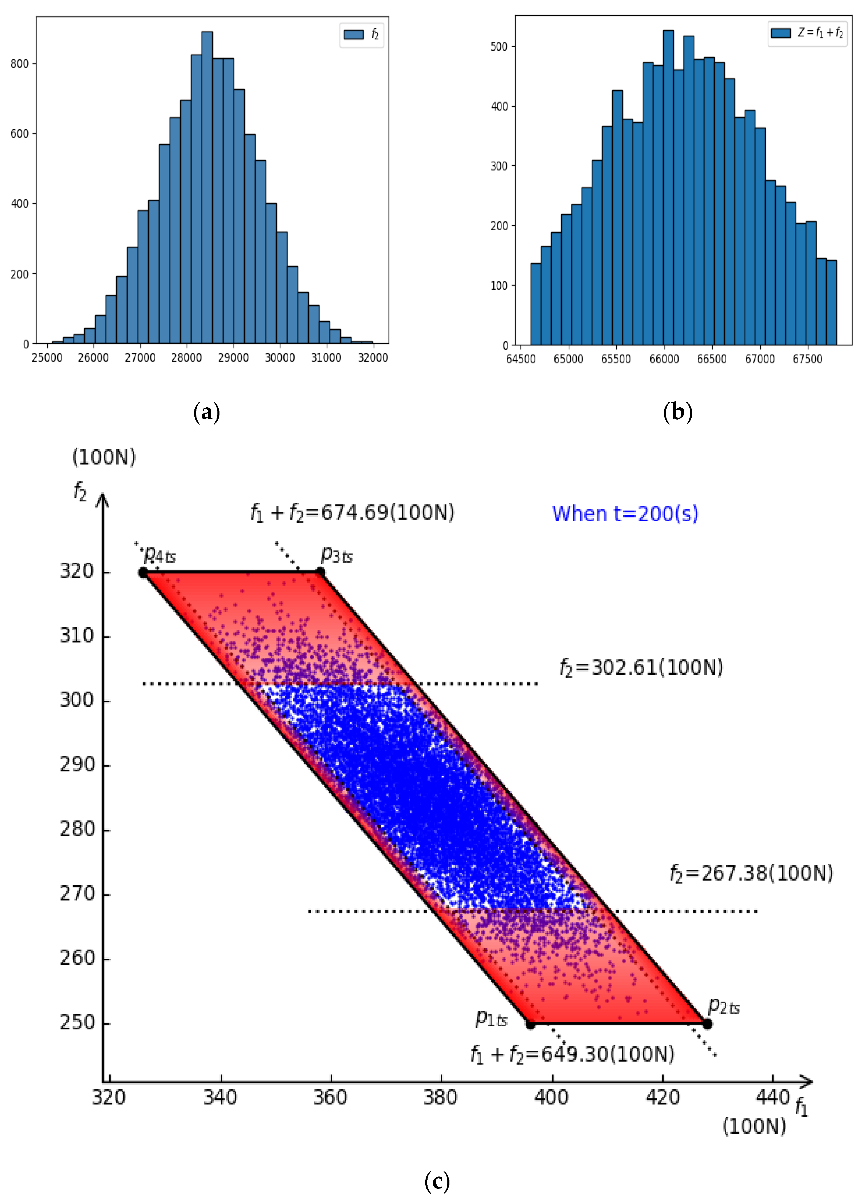
4.2. Simulation and Test

The three truncated normal intervals in $\overline{\phi }$ are, $M_1=[50,000,60,000{]}_{h_1}$, $\zeta ={[1.5,2]}_{h_{\zeta }}$ and $f_{12}={[0,2000]}_{h_{f12}}$ $h_1$,$h_{\zeta }$,$h_{f_{12}}$ and are the probability density functions. According to acceptance–rejection sampling, when $t=t_s$, we can obtain n groups of test cases, denoted as $cas{e}_i=[{(M_1)}_i,{\zeta }_i,{(f_{12})}_i],i=1,2,\dots n$. Taking $cas{e}_i=[{(M_1)}_i,{\zeta }_i,{(f_{12})}_i],i=1,2,\dots n$ into formula (20), the n solutions ($solutio{n}_i=[{(f_1)}_i,{(f_2)}_i]$) can be obtained. We can then count the distributions of these solutions. Figure 10a,b show the distributions of f₂ and $Z=f_1+f_2$ in their truncated intervals, respectively, when n = 10,000; Figure 10c shows the distribution of that when t = 200.

Algorithm 1 is given below for generating simulation cases and distribution values of $f_1$ and $f_2$ when t ranges from 1 to 200.

Algorithm 1 used to generate simulation cases

1: begin

2: t = 1, $\Delta t=1$; 3: while (t <= 200)     begin while

4:  Generate n cases $(cas{e}_i=[{(M_1)}_i,{\zeta }_i,{(f_{12})}_i],i=1,2,\dots n$), according to acceptance –rejection sampling;   5:  Take $cas{e}_i=[{(M_1)}_i,{\zeta }_i,{(f_{12})}_i],i=1,2,\dots n$ into formula (20),      then calculate them and obtain $solutio{n}_i=[{(f_1)}_i,{(f_2)}_i], i=1,2,\dots n$;

6:   $t=t+\Delta t$;  end while

7: end

From the above algorithm, taking n = 100 for every discrete integer t value, $t=1,2,\dots ,200$, we can obtain Figure 11, where the power distributions of $f_1$ and are $f_2$ represented by the blue points.

According to step 3 and step 4 of the reasoning method given in Section 3.2, we obtain the following: during the acceleration, if it is found that the power distribution of $f_1$ and $f_2$ are not within the area enclosed by “$P_1{P}_2{P}_3{P}_4{P}_5{P}_6{P}_7{P}_8$” in Figure 11, it means that there must be non-error factors affecting the power system, and fault detection should be carried out immediately; if the power distributions of $f_1$ and $f_2$ are inside the area “$P_1{P}_2{P}_3{P}_4{P}_5{P}_6{P}_7{P}_8$” in Figure 11, and if $f_1$ and $f_2$ continuously appear inside the red area of Figure 11, according to statistics, there is a high probability that non-error factors affect the system in the train power system at this time; fault detection is still required immediately.

From Figure 11, most of the distributions of $f_1$ and $f_2$ are inside the white area.

5. Discussion

Previous reasoning methods have mainly focused on systems with precise parameters. Most of these are invalid for systems with uncertain parameters because the Gröbner basis changes discontinuously with coefficients. The authors proposed some reasoning methods [20,21,22] for systems with uncertain parameters. Power distribution areas caused by error parameters can be obtained, and it can be used to determine whether the system has non-error fault factors (mechanical and electrical faults) by observing whether the system states are inside the area, but these methods ignore the probability information of the errors within the interval. The method proposed in this paper combines the probability information of errors with previous reasoning methods. Hence, not only can the power distribution areas be obtained, but also an area divided area by statistics, by which it can be earlier determined whether there are non-error fault factors compared with the methods [20,21,22]. Hence, the results obtained by this method are more complete than those of the methods [20,21]. Nevertheless, the method in this paper involves more calculations than the methods [20,21]. Finally, it is noteworthy while that this method increases the complexity of the calculation, it is necessary for safety-critical systems. Some scholars have studied based-fuzzy logic [30] reasoning rules [31], which have been applied in some aspects [32,33]. These are different from those of our method. Our method has a more obvious statistical significance.

Table 1. Advantages and disadvantages of this method and other methods.

Methods	Advantage	Disadvantage
Methods [20,21] (linear error assertions)	Better time complexity compared to other methods in the table.	May be invalid for non-convex zero set; Lack of error probability information.
Method [22] (error polynomial assertions)	Valid for non-convex zero set.	Very high time complexity; Lack of error probability information.
Method [30] (fuzzy reasoning)	Based on fuzzy logic; it has well-established theoretical support.	Weak statistical significance.
The method in this article	Strong statistical significance. Identifies potential faults earlier than methods [20,21].	Higher time complexity than that of the methods [20,21].

shows the advantages and disadvantages of this method and other reasoning methods.

6. Conclusions

Our main contributions are as follows: First, the errors were represented by symmetric truncated normal intervals, and the probability information of the errors was described by a truncated normal probability density function. Lemmas 1, 2 and Theorem 1 and their proofs are provided, which partially simplify the calculations between truncated normal intervals. Second, we combined symmetric truncated normal intervals with the previous reasoning methods and provided the steps of the reasoning method. The calculation of probability information is added to the reasoning method, which makes the reasoning method more effective and valuable than the method in [20,21,22] for safety-critical systems. Finally, a reasonable example of train acceleration was provided. Most of the points were inside the white area in Figure 11, which indicates that the theoretical calculation results (the white area comes from the reasoning method in this article) was consistent with the simulation results in this example.

References

1. Fisher, M.; Cardoso, R.C.; Collins, E.C.; Dadswell, C.; Dennis, L.A.; Dixon, C.; Farrell, M.; Ferrando, A.; Huang, X.; Jump, M.; et al. An Overview of Verification and Validation Challenges for Inspection Robots. Robotics 2021, 10, 67. [Google Scholar] [CrossRef]
2. Sun, M.; Lu, Y.; Feng, Y.; Zhang, Q.; Liu, S. Modeling and Verifying the CKB Blockchain Consensus Protocol. Mathematics 2021, 9, 2954. [Google Scholar] [CrossRef]
3. Wang, J.; Zhan, N.J.; Feng, X.Y.; Liu, Z.M. Overview of formal methods. J. Softw. 2019, 30, 33–61. [Google Scholar]
4. Clarke, E.M.; Henzinger, T.A.; Veith, H.; Bloem, R. Handbook of Model Checking; Springer: Cham, Switzerland, 2018; Chapter 12; ISBN 9783030132330. [Google Scholar]
5. Desai, A.; Dreossi, T.; Seshia, S.A. Combining Model Checking and Runtime Verification for Safe Robotics. In Runtime Verification, Proceedings of the International Conference on Runtime Verification, Seattle, WA, USA, 13–16 September 2017; Springer: Berlin/Heidelberg, Germany, 2017; pp. 172–189. [Google Scholar] [CrossRef]
6. Uribe, T.E. Combinations of model checking and theorem proving. In Proceedings of the International Workshop on Frontiers of Combining Systems, Nancy, France, 22–24 March 2000; pp. 151–170. [Google Scholar]
7. Shankar, N. Combining theorem proving and model checking through symbolic analysis. Int. Conf. Concurr. Theory 2000, 1877, 1–16. [Google Scholar]
8. Wu, J. Algebraic methods for mechanical theorem proving in many-valued logics. Chin. J. Comput. 1996, 10, 773–779. [Google Scholar]
9. Fu, J.; Wu, J.; Tan, H. A deductive approach towards reasoning about algebraic transition systems. Math. Probl. Eng. 2015, 607013. [Google Scholar] [CrossRef]
10. Platzer, A. Logical Analysis of Hybrid Systems: Proving Theorems for Complex Dynamics; Springer Science & Business Media: Berlin/Heidelberg, Germany, 2010; ISBN 9783642145087. [Google Scholar]
11. Liu, J.; Zhan, N.; Zhao, H. Computing semi-algebraic invariants for polynomial dynamical systems. In Proceedings of the Ninth ACM International Conference on Embedded Software, Taipei, Taiwan, 9–14 October 2011; pp. 97–106. [Google Scholar]
12. Elias, J. Automated Geometric Theorem Proving: Wu’s Method. Master’s Thesis, University of Montana, Missoula, MT, USA, 2006. [Google Scholar] [CrossRef]
13. Buchberger, B. Gröbner bases: An algorithmic method in polynomial ideal theory. Multidimens. Syst. Theory 1995, 89–127. [Google Scholar] [CrossRef]
14. Arnon, D.S.; Collins, G.E.; McCallum, S. Cylindrical algebraic decomposition. I. The basic algorithm. SIAM J. Comput. 1984, 13, 865–877. [Google Scholar] [CrossRef] [Green Version]
15. Wang, D. Elimination Methods. Springer: Wien, Austria, 2001; ISBN 9783709162026. [Google Scholar]
16. Fulton, N.; Mitsch, S.; Quesel, J.D.; Völp, M.; Platzer, A. KeYmaera X: An axiomatic tactical theorem prover for hybrid systems. In Proceedings of the Conference on Automated Deduction, Berlin, Germany, 1–7 August 2015; pp. 527–538. [Google Scholar] [CrossRef]
17. Hunt, W.A.; Kaufmann, M.; Strother, M.J.; Slobodova, A. Industrial hardware and software verification with acl2. Philos. Trans. R. Soc. A 2017, 375, 20150399. [Google Scholar] [CrossRef] [PubMed]
18. Chatterjee, K.; Zavadskas, E.K.; Tamošaitienė, J.; Adhikary, K.; Kar, S. A Hybrid MCDM Technique for Risk Management in Construction Projects. Symmetry 2018, 10, 46. [Google Scholar] [CrossRef] [Green Version]
19. Kondratyev, A.; Stetter, H.J.; Winkler, S. Numerical computation of Gröbner bases. In Proceedings of the CASC2004 (Computer Algebra in Scientific Computing), Chişinău, Moldova, 11–15 September 2004; pp. 295–306. [Google Scholar]
20. Wu, P.; Xiong, N.; Liu, J.; Huang, L.; Ju, Z.; Ji, Y.; Wu, J. Interval number-based safety reasoning method for verification of decentralized power systems in high-speed trains. Math. Probl. Eng. 2021, 6624528. [Google Scholar] [CrossRef]
21. Wu, P.; Wu, J. Reasoning method based on linear error assertion. J. Comput. Appl. 2021, 41, 2199–2204. [Google Scholar] [CrossRef]
22. Wu, P.; Xiong, N.; Xiong, J.; Wu, J. Reasoning method between polynomial error assertions. Information 2021, 12, 309. [Google Scholar] [CrossRef]
23. Burkardt, J. The Truncated Normal Distribution. Available online: https://people.sc.fsu.edu/~jburkardt/presentations/truncated_normal.pdf. (accessed on 16 November 2021).
24. Robert, C.P. Simulation of truncated normal variables. Stat. Comput. 1995, 5, 121–125. [Google Scholar] [CrossRef] [Green Version]
25. Castillo, N.O.; Gallardo, D.I.; Bolfarine, H.; Gómez, H.W. Truncated Power-Normal Distribution with Application to Non-Negative Measurements. Entropy 2018, 20, 433. [Google Scholar] [CrossRef] [PubMed] [Green Version]
26. Barr, D.; Sherrill, E. Mean and variance of truncated normal distributions. Am. Stat. 1999, 53, 357–361. [Google Scholar]
27. Shoenfield, J.R. Mathematical Logic; AK Peters/CRC Press: Natick, MA, USA, 2001; ISBN 1568811357. [Google Scholar]
28. Csörgő, M. Quantile Processes with Statistical Applications; Society for Industrial and Applied Mathematics: Philadelphia, PA, USA, 1983; ISBN 0898711851. [Google Scholar]
29. Volgushev, S.; Chao, S.-K.; Cheng, G. Distributed inference for quantile regression processes. Ann. Stat. 2019, 47, 1634–1662. [Google Scholar] [CrossRef] [Green Version]
30. Belohlavek, R.; Dauben, J.W.; Klir, G.J. Fuzzy Logic and Mathematics: A Historical Perspective; Oxford University Press: Oxford, UK, 2017; ISBN 9780190200015. [Google Scholar]
31. Nazari, S.; Fallah, M.; Kazemipoor, H.; Salehipour, A. A fuzzy inference-fuzzy analytic hierarchy process-based clinical decision support system for diagnosis of heart diseases. Expert Syst. Appl. 2018, 95, 261–271. [Google Scholar] [CrossRef]
32. Mehrabi, M.; Pradhan, B.; Moayedi, H.; Alamri, A. Optimizing an Adaptive Neuro-Fuzzy Inference System for Spatial Prediction of Landslide Susceptibility Using Four State-of-the-art Metaheuristic Techniques. Sensors 2020, 20, 1723. [Google Scholar] [CrossRef] [PubMed] [Green Version]
33. Lin, H.; Liu, X.; Wang, X.; Liu, Y. A fuzzy inference and big data analysis algorithm for the prediction of forest fire based on rechargeable wireless sensor networks. Sustain. Comput. Infor. Syst. 2018, 18, 101–111. [Google Scholar] [CrossRef]
Figure 1. Example of truncated normal density.
Symmetry 14 00025 g001
Figure 2. Example of normal probability density function.
Symmetry 14 00025 g002
Figure 3. Transition of train states.
Symmetry 14 00025 g003
Figure 4. Power distribution of the two bodies with the smoothly accelerating.
Symmetry 14 00025 g004
Figure 5. Power distribution domain when t = ts (the interior surrounded by black lines).
Symmetry 14 00025 g005
Figure 6. Horizontal section of power distribution domain when t = ts.
Symmetry 14 00025 g006
Figure 7. Division of Z e r o ( φ ¯ ) when t = 150.
Symmetry 14 00025 g007
Figure 8. Division of Z e r o ( φ ¯ ) when t = 200.
Symmetry 14 00025 g008
Figure 9. Division of Z e r o ( φ ¯ ) when t ∈ [0,200].
Symmetry 14 00025 g009
Figure 10. (a) Distributions of f2 when n = 10,000 and t = 200; (b) The distributions of Z = f1 + f2 when n = 10,000 and t = 200; (c) The distributions of s o l u t i o n i (i = 1, …, 10,000) when t = 200.
Symmetry 14 00025 g010
Figure 11. Division of Z e r o ( φ ¯ ) when t ∈ [0,200].
Symmetry 14 00025 g011