A Quadruple Integral Involving Product of the Struve H_v(βt) and Parabolic Cylinder D_u(αx) Functions

Abstract

The objective of the present paper is to obtain a quadruple infinite integral. This integral involves the product of the Struve and parabolic cylinder functions and expresses it in terms of the Hurwitz–Lerch Zeta function. Almost all Hurwitz-Lerch Zeta functions have an asymmetrical zero distributionSpecial cases in terms fundamental constants and other special functions are produced. All the results in the work are new.

1. Significance Statement

In 1927, Watson et al. [1] published work on the infinite integral involving the product of the Struve ${\mathit{H}}_v\left(\beta t\right)$ and parabolic cylinder $D_u\left(\alpha x\right)$ functions expressed in terms of the quotient of gamma functions. In 1945, Mitra [2] extended the work achieved by Watson et al. by deriving and evaluating other forms of these infinite integrals involving the product of Struve and parabolic cylinder functions. In this current work, we take this previous important work a step further by deriving a quadruple definite integral involving these special functions. We will derive a quadruple integral and express in terms of a Hurwitz–Lerch Zeta function. Special cases are derived in terms of the Polylogarithm function $L{i}_k\left(z\right)$, Catalan’s constant C, Hurwitz Zeta function $\zeta (s,v)$, the Harmonic function $H_n$, the Zeta function of Riemann $\zeta \left(k\right)$, and $log\left(2\right)$. An interesting invariant property of the indices in the Struve ${\mathit{H}}_v\left(\beta t\right)$ and parabolic cylinder $D_u\left(\alpha x\right)$ functions is evaluated. This invariant property, related to multiple integrals, is a new topic to the best of our knowledge. We will be investigating this property along with other multiple integrals in future work. We will be looking at any similarities this property has to multiple definite integral of these functions and any real world applications which they possess.

2. Introduction

In this paper we derive the quadruple definite integral given by:

$$\begin{array}{c}{\int }_0^{\infty }{\int }_0^{\infty }{\int }_0^{\infty }{\int }_0^{\infty }{x}^{-m/2}{t}^{m-v-1}{y}^{-\frac{m}{2}-u+1}{z}^{-m+2v+1}{D}_u\left(x\alpha \right){\mathit{H}}_v\left(t\beta \right)\hfill \\ \hfill e^{-b\left(y^2+z^2\right)-\frac{1}{4}{\alpha }^2{x}^2}{log}^k\left(\frac{at}{\sqrt{x}\sqrt{y}z}\right)dxdydzdt\end{array}$$

(1)

where the parameters $k,a,\alpha ,\beta ,u,v,$ and m are general complex numbers and $Re\left(u\right)<Re\left(m\right)<1/2,Re\left(m\right)<Re\left(v\right)$. This definite integral will be used to derive special cases in terms of special functions and fundamental constants. The derivations follow the method used by us in [3]. This method involves using a form of the generalized Cauchy’s integral formula given by:

$$\frac{y^k}{\Gamma (k+1)}=\frac{1}{2\pi i}{\int }_C\frac{e^{wy}}{w^{k+1}}dw.$$

(2)

where C is, in general, an open contour in the complex plane where the bilinear concomitant has the same value at the end points of the contour. We then multiply both sides by a function of x, y, z, and t, then take a definite quadruple integral of both sides. This yields a definite integral in terms of a contour integral. Then, we multiply both sides of Equation (2) by another function of x, y, z, and t and take the infinite sums of both sides such that the contour integral of both equations are the same.

3. Definite Integral of the Contour Integral

We used the method in [3]. The variable of integration in the contour integral is $r=w+m$. The cut and contour are in the first quadrant of the complex r-plane. The cut approaches the origin from the interior of the first quadrant; the contour goes round the origin with zero radius and is on opposite sides of the cut. Using a generalization of Cauchy’s integral formula, we form the quadruple integral by replacing y with $log\left(\frac{at}{\sqrt{x}\sqrt{y}z}\right)$ and multiplying by $x^{-m/2}{t}^{m-v-1}{y}^{-\frac{m}{2}-u+1}{z}^{-m+2v+1}{D}_u\left(x\alpha \right){\mathit{H}}_v\left(t\beta \right)e^{-b\left(y^2+z^2\right)-\frac{1}{4}{\alpha }^2{x}^2}$, then taking the definite integral with respect to $x\in (0,\infty )$, $y\in (0,\infty )$, $z\in (0,\infty )$, and $t\in (0,\infty )$ to obtain

$$\begin{array}{c}\frac{1}{\Gamma (k+1)}{\int }_0^{\infty }{\int }_0^{\infty }{\int }_0^{\infty }{\int }_0^{\infty }{x}^{-m/2}{t}^{m-v-1}{y}^{-\frac{m}{2}-u+1}{z}^{-m+2v+1}\hfill \\ \hspace{1em}\hspace{1em}\hspace{1em}\hspace{1em}{D}_u\left(x\alpha \right){\mathit{H}}_v\left(t\beta \right)e^{-b\left(y^2+z^2\right)-\frac{1}{4}{\alpha }^2{x}^2}{log}^k\left(\frac{at}{\sqrt{x}\sqrt{y}z}\right)dxdydzdt\\ \\ \hspace{1em}\hspace{1em}\hspace{1em}=\frac{1}{2\pi i}{\int }_0^{\infty }{\int }_0^{\infty }{\int }_0^{\infty }{\int }_0^{\infty }{\int }_C{a}^w{w}^{-k-1}{x}^{\frac{1}{2}(-m-w)}{t}^{m-v+w-1}{y}^{\frac{1}{2}(-m-w)-u+1}\\ z^{-m+2v-w+1}{D}_u\left(x\alpha \right){\mathit{H}}_v\left(t\beta \right)e^{-b\left(y^2+z^2\right)-\frac{1}{4}{\alpha }^2{x}^2}dwdxdydzdt\\ \\ \hspace{1em}\hspace{1em}\hspace{1em}=\frac{1}{2\pi i}{\int }_C{\int }_0^{\infty }{\int }_0^{\infty }{\int }_0^{\infty }{\int }_0^{\infty }{a}^w{w}^{-k-1}{x}^{\frac{1}{2}(-m-w)}{t}^{m-v+w-1}{y}^{\frac{1}{2}(-m-w)-u+1}\\ z^{-m+2v-w+1}{D}_u\left(x\alpha \right){\mathit{H}}_v\left(t\beta \right)e^{-b\left(y^2+z^2\right)-\frac{1}{4}{\alpha }^2{x}^2}dxdydzdtdw\\ \\ \hspace{1em}\hspace{1em}\hspace{1em}=\frac{1}{2\pi i}{\int }_C{\pi }^{3/2}{a}^w{w}^{-k-1}{\alpha }^{\frac{m+w}{2}-1}sec\left(\frac{1}{2}\pi (m+w)\right)2^{\frac{1}{4}(5(m+w)+2(u-2v-7))}\\ \hfill {\beta }^{-m+v-w}{b}^{\frac{3(m+w)}{4}+\frac{u}{2}-v-2}dw\end{array}$$

(3)

from Equation (3.326.2) in [4], equations (3.9.1.3) and (3.15.1) in [5] where $Re\left(\beta \right)>0,0<Re(w+m)<3/2,\left|Re\right(w+m+\beta \left)\right|<1,|arg\alpha |<\pi /4$, and using the reflection formula (8.334.3) in [4] for the Gamma function. We are able to switch the order of integration over x, y, z, and t using Fubini’s theorem for multiple integrals see (9.112) in [6], as the integrand is of bounded measure over the space $\mathbb{C}\times (0,\infty )\times (0,\infty )\times (0,\infty )\times (0,\infty )$.

4. The Hurwitz–Lerch Zeta Function and Infinite Sum of the Contour Integral

In this section we use Equation (2) to derive the contour integral representations for the Hurwitz–Lerch Zeta function.

4.1. The Hurwitz–Lerch Zeta Function

The Hurwitz–Lerch Zeta function (25.14) in [7] and [8] has a series representation given by

$$\Phi (z,s,v)=\sum _{n=0}^{\infty }{(v+n)}^{-s}{z}^n$$

(4)

where $\left|z\right|<1,v\ne 0,-1,..$ and is continued analytically by its integral representation given by

$$\Phi (z,s,v)=\frac{1}{\Gamma \left(s\right)}{\int }_0^{\infty }\frac{t^{s-1}{e}^{-vt}}{1-z{e}^{-t}}dt=\frac{1}{\Gamma \left(s\right)}{\int }_0^{\infty }\frac{t^{s-1}{e}^{-(v-1)t}}{e^t-z}dt$$

(5)

where $Re\left(v\right)>0$, and either $\left|z\right|\le 1,z\ne 1,Re\left(s\right)>0$, or $z=1,Re\left(s\right)>1$.

4.2. Infinite Sum of the Contour Integral

Using Equation (2) and replacing y with $log\left(a\right)+\frac{log\left(\alpha \right)}{2}+\frac{3log\left(b\right)}{4}-log\left(\beta \right)+\frac{1}{2}i\pi (2y+1)+\frac{5log\left(2\right)}{4}$, then multiplying both sides by ${\pi }^{3/2}{(-1)}^y{\alpha }^{\frac{m}{2}-1}{e}^{\frac{1}{2}i\pi m(2y+1)}{2}^{\frac{1}{4}(5m+2(u-2v-7))+1}$${\beta }^{v-m}{b}^{\frac{3m}{4}+\frac{u}{2}-v-2}$, taking the infinite sum over $y\in [0,\infty )$, and simplifying in terms of the Hurwitz–Lerch Zeta function we obtain

$$\begin{array}{c}\frac{1}{\Gamma (k+1)}{\pi }^{k+\frac{3}{2}}{e}^{\frac{1}{2}i\pi (k+m)}{\alpha }^{\frac{m}{2}-1}{2}^{\frac{1}{4}(5m+2(u-2v-5))}{\beta }^{v-m}{b}^{\frac{3m}{4}+\frac{u}{2}-v-2}\hfill \\ \Phi \left(-e^{im\pi },-k,\frac{i(-4log(a)-3log(b)-2log(\alpha )+4log(\beta )-5log(2)-2i\pi )}{4\pi }\right)\\ \\ =\frac{1}{2\pi i}\sum _{y=0}^{\infty }{\int }_C{\pi }^{3/2}{(-1)}^y{w}^{-k-1}{\alpha }^{\frac{m}{2}-1}{\beta }^{v-m}{b}^{\frac{3m}{4}+\frac{u}{2}-v-2}{2}^{\frac{1}{4}(5m+2u-4v+5w-10)}\\ exp\left(\frac{1}{4}(w(4log\left(a\right)+2log\left(\alpha \right)+3log\left(b\right)-4log\left(\beta \right))+2i\pi (2y+1)(m+w))\right)dw\\ \\ =\frac{1}{2\pi i}{\int }_C\sum _{y=0}^{\infty }{\pi }^{3/2}{(-1)}^y{w}^{-k-1}{\alpha }^{\frac{m}{2}-1}{\beta }^{v-m}{b}^{\frac{3m}{4}+\frac{u}{2}-v-2}{2}^{\frac{1}{4}(5m+2u-4v+5w-10)}\\ exp\left(\frac{1}{4}(w(4log\left(a\right)+2log\left(\alpha \right)+3log\left(b\right)-4log\left(\beta \right))+2i\pi (2y+1)(m+w))\right)dw\\ \\ =\frac{1}{2\pi i}{\int }_C{\pi }^{3/2}{a}^w{w}^{-k-1}{\alpha }^{\frac{1}{2}(m+w-2)}sec\left(\frac{1}{2}\pi (m+w)\right)\\ \hfill 2^{\frac{1}{4}(5m+2u-4v+5w-14)}{\beta }^{-m+v-w}{b}^{\frac{1}{4}(3m+2u-4v+3w-8)}dw\end{array}$$

(6)

from Equation (1.232.2) in [4] where $Im\left(\frac{\pi }{2}(m+w)\right)>0$ in order for the sum to converge.

5. Definite Integral in Terms of the Hurwitz–Lerch Zeta Function

Theorem 1.

For all $k,a,\alpha ,\beta ,u,v,m\in \mathbb{C},Re\left(b\right)>0,Re\left(u\right)<Re\left(m\right)<1/2$, and $Re\left(m\right)<Re\left(v\right)$, then

$$\begin{array}{c}{\int }_0^{\infty }{\int }_0^{\infty }{\int }_0^{\infty }{\int }_0^{\infty }{x}^{-m/2}{t}^{m-v-1}{y}^{-\frac{m}{2}-u+1}{z}^{-m+2v+1}{D}_u\left(x\alpha \right){\mathit{H}}_v\left(t\beta \right)\hfill \\ e^{-b\left(y^2+z^2\right)-\frac{1}{4}{\alpha }^2{x}^2}{log}^k\left(\frac{at}{\sqrt{x}\sqrt{y}z}\right)dxdydzdt\\ ={\pi }^{k+\frac{3}{2}}{e}^{\frac{1}{2}i\pi (k+m)}{\alpha }^{\frac{m}{2}-1}{2}^{\frac{1}{4}(5m+2(u-2v-5))}{\beta }^{v-m}{b}^{\frac{3m}{4}+\frac{u}{2}-v-2}\\ \hfill \Phi \left(-e^{im\pi },-k,\frac{i(-4log(a)-3log(b)-2log(\alpha )+4log(\beta )-5log(2)-2i\pi )}{4\pi }\right)\end{array}$$

(7)

Proof. 

The right-hand sides of relations (3) and (6) are identical; hence, the left-hand sides of the same are identical too. Simplifying with the Gamma function yields the desired conclusion. □

Example 1.

The degenerate case

$$\begin{array}{c}{\int }_0^{\infty }{\int }_0^{\infty }{\int }_0^{\infty }{\int }_0^{\infty }{x}^{-m/2}{t}^{m-v-1}{2}^{\frac{1}{4}(5m+2(u-2v-5))}{y}^{-\frac{m}{2}-u+1}{z}^{-m+2v+1}{b}^{\frac{3m}{4}+\frac{u}{2}-v-2}\hfill \\ D_u\left(x\alpha \right){\mathit{H}}_v\left(t\beta \right)e^{-b\left(y^2+z^2\right)-\frac{1}{4}{\alpha }^2{x}^2}dxdydzdt\\ \hfill ={\pi }^{3/2}{\alpha }^{\frac{m}{2}-1}sec\left(\frac{\pi m}{2}\right)2^{\frac{1}{4}(5m+2(u-2v-7))}{\beta }^{v-m}{b}^{\frac{3m}{4}+\frac{u}{2}-v-2}\end{array}$$

(8)

Proof. 

Use Equation (7) and set $k=0$ and simplify using entry (2) in Table below (64:12:7) in [9]. □

Example 2.

The Polylogarithm function $L{i}_k\left(z\right)$

$$\begin{array}{c}{\int }_0^{\infty }{\int }_0^{\infty }{\int }_0^{\infty }{\int }_0^{\infty }{x}^{-m/2}{t}^{m-v-1}{y}^{-\frac{m}{2}-u+1}{z}^{-m+2v+1}{D}_u\left(\frac{x}{2}\right)\hfill \\ {\mathit{H}}_v\left(2t\right)e^{-\frac{x^2}{16}-\sqrt[3]{2}\left(y^2+z^2\right)}{log}^k\left(\frac{it}{\sqrt{x}\sqrt{y}z}\right)dxdydzdt\\ ={\pi }^{k+\frac{3}{2}}{e}^{\frac{1}{2}i\pi (k+m)-i\pi m}{\mathrm{Li}}_{-k}\left(-e^{im\pi }\right)\\ \hfill \left(-2^{\frac{1}{4}(5m+2(u-2v-5))+\frac{1}{3}\left(\frac{3m}{4}+\frac{u}{2}-v-2\right)-\frac{3m}{2}+v+1}\right)\end{array}$$

(9)

Proof. 

Use Equation (7) and set $a=i,\beta =2,b=2^{1/3},\alpha =1/2$ simplify using Equation (64:12:2) in [9]. □

Example 3.

Catalan’s constant C

$$\begin{array}{c}{\int }_0^{\infty }{\int }_0^{\infty }{\int }_0^{\infty }{\int }_0^{\infty }\frac{t^{-v-\frac{1}{2}}{y}^{\frac{3}{4}-u}{z}^{2v+\frac{1}{2}}{D}_u\left(\frac{x}{2}\right){\mathit{H}}_v\left(2t\right)e^{-\frac{x^2}{16}-\sqrt[3]{2}\left(y^2+z^2\right)}}{\sqrt[4]{x}{log}^2\left(\frac{it}{\sqrt{x}\sqrt{y}z}\right)}dxdydzdt\hfill \\ \hfill =\frac{{(-1)}^{3/4}\left({\pi }^2+48iC\right)2^{\frac{1}{6}(4u-2v-37)}}{3\sqrt{\pi }}\end{array}$$

(10)

Proof. 

Use Equation (9) and set $k=-2,m=1/2$ and simplify using Equation (2.1.2.2.7) in [10]. □

6. The Invariance of Indices $\mathit{u}$ and $\mathit{v}$ Relative to the Hurwitz–Lerch Zeta Function

In this section, we evaluate Equation (7) such that the indices of the Struve ${\mathit{H}}_v\left(\beta t\right)$ and parabolic cylinder $D_u\left(\alpha x\right)$ functions are independent of the right-hand side. These types of integrals could involve properties related to orthogonal functions. This invariant property occurs as a result of how the gamma function is chosen for the definite integral of the contour integral to reduce to a trigonometric function. The derivation of this invariant property is not dependent on all the parameters involved.

Example 4.

The Polylogarihm function $L{i}_k\left(z\right)$

$$\begin{array}{c}{\int }_0^{\infty }{\int }_0^{\infty }{\int }_0^{\infty }{\int }_0^{\infty }{x}^{-m/2}{t}^{m-v-1}{y}^{-\frac{m}{2}-u+1}{z}^{-m+2v+1}{D}_u\left(\frac{x}{2}\right)\hfill \\ {\mathit{H}}_v\left(t\right)e^{\frac{1}{16}\left(-x^2-8\left(y^2+z^2\right)\right)}{log}^k\left(\frac{it}{\sqrt{x}\sqrt{y}z}\right)dxdydzdt\\ \hfill =-\sqrt{2}{\pi }^{k+\frac{3}{2}}{e}^{\frac{1}{2}i\pi (k-m)}{\mathrm{Li}}_{-k}\left(-e^{im\pi }\right)\end{array}$$

(11)

Proof. 

Use Equation (7) and set $a=i,\beta =1,b=1/2,\alpha =1/2$; simplify using Equation (64:12:2) in [9]. □

Example 5.

The inverse hyperbolic cosine function ${cosh}^{-1}\left(x\right)$

$$\begin{array}{c}{\int }_0^{\infty }{\int }_0^{\infty }{\int }_0^{\infty }{\int }_0^{\infty }\frac{t^{-v-\frac{3}{5}}{y}^{\frac{4}{5}-u}{z}^{2v+\frac{3}{5}}{D}_u\left(\frac{x}{2}\right){\mathit{H}}_v\left(t\right)e^{\frac{1}{16}\left(-x^2-8\left(y^2+z^2\right)\right)}}{\sqrt[5]{x}log\left(\frac{it}{\sqrt{x}\sqrt{y}z}\right)}dxdydzdt\hfill \\ \hfill =\frac{1}{40}\left(\sqrt{2\pi }+\sqrt{10\pi }-2i\sqrt{\left(5-\sqrt{5}\right)\pi }\right)\left(2\pi -5i{cosh}^{-1}\left(\frac{3}{2}\right)\right)\end{array}$$

(12)

Proof. 

Use Equation (11) and set $k=-1,m=2/5$ and simplify. □

Example 6.

The Hurwitz Zeta function $\zeta (s,v)$

$$\begin{array}{c}{\int }_0^{\infty }{\int }_0^{\infty }{\int }_0^{\infty }{\int }_0^{\infty }{t}^{-v-1}{y}^{1-u}{z}^{2v+1}{D}_u\left(\frac{x}{4}\right){\mathit{H}}_v\left(t\right)e^{\frac{1}{64}\left(-x^2-32\left(y^2+z^2\right)\right)}\hfill \\ {log}^k\left(\frac{it}{\sqrt{x}\sqrt{y}z}\right)dxdydzdt\\ \hfill =e^{\frac{i\pi k}{2}}{\left(2\pi \right)}^{k+\frac{3}{2}}\left(\zeta \left(-k,\frac{1}{2}+\frac{ilog\left(2\right)}{4\pi }\right)-\zeta \left(-k,1+\frac{ilog\left(2\right)}{4\pi }\right)\right)\end{array}$$

(13)

Proof. 

Use Equation (7) and set $m=0,a=i,b=1/2,\alpha =1/4,\beta =1$ and simplify using entry (4) in Table below (64:12:70) in [9]. □

Example 7.

The Harmonic number function $H_n$

$$\begin{array}{c}{\int }_0^{\infty }{\int }_0^{\infty }{\int }_0^{\infty }{\int }_0^{\infty }\frac{y^{4/3}{z}^7{D}_{-\frac{1}{3}}\left(\frac{x}{4}\right){\mathit{H}}_3\left(t\right)e^{\frac{1}{64}\left(-x^2-32\left(y^2+z^2\right)\right)}}{t^{4}log\left(\frac{it}{\sqrt{x}\sqrt{y}z}\right)}dxdydzdt\hfill \\ \hfill =-i\sqrt{2\pi }\left(H_{\frac{ilog\left(2\right)}{4\pi }}-H_{-\frac{1}{2}+\frac{ilog\left(2\right)}{4\pi }}\right)\end{array}$$

(14)

Proof. 

Use Equation (13) and set $u=-1/3,v=3$ and apply l’Hopital’s rule as $k\to -1$ and simplify using Equation (14) in [11]. □

Example 8.

The Zeta function of Riemann $\zeta \left(k\right)$

$$\begin{array}{c}{\int }_0^{\infty }{\int }_0^{\infty }{\int }_0^{\infty }{\int }_0^{\infty }{t}^{-v-1}{y}^{1-u}{z}^{2v+1}{D}_u\left(\frac{x}{2}\right){\mathit{H}}_v\left(t\right)e^{\frac{1}{16}\left(-x^2-8\left(y^2+z^2\right)\right)}{log}^k\left(\frac{it}{\sqrt{x}\sqrt{y}z}\right)dxdydzdt\hfill \\ \hfill =-\sqrt{2}\left(2^{k+1}-1\right)e^{\frac{i\pi k}{2}}{\pi }^{k+\frac{3}{2}}\zeta (-k)\end{array}$$

(15)

Proof. 

Use Equation (7) and set $a=i,m=0,b=1/2,\beta =1,\alpha =1/2$ and simplify using entry (4) in Table below (64:12:7) and entry (2) in table (64:7) in [9]. □

Example 9.

The fundamental constant $log\left(2\right)$

$$\begin{array}{c}{\int }_0^{\infty }{\int }_0^{\infty }{\int }_0^{\infty }{\int }_0^{\infty }\frac{t^{-v-1}{y}^{1-u}{z}^{2v+1}{D}_u\left(\frac{x}{2}\right){\mathit{H}}_v\left(t\right)e^{\frac{1}{16}\left(-x^2-8\left(y^2+z^2\right)\right)}}{log\left(\frac{it}{\sqrt{x}\sqrt{y}z}\right)}dxdydzdt\hfill \\ \hspace{1em}\hspace{1em}\hspace{1em}\hspace{1em}\hspace{1em}\hspace{1em}\hspace{1em}=-i\sqrt{2\pi }log\left(2\right)\end{array}$$

(16)

Proof. 

Use Equation (15) and apply l’Hopitals’ rule as $k\to -1$ and simplify using Equation (25.6.11) in [7]. □

Example 10.

Apéry’s constant $\zeta \left(3\right)$

$$\begin{array}{c}{\int }_0^{\infty }{\int }_0^{\infty }{\int }_0^{\infty }{\int }_0^{\infty }\frac{t^{-v-1}{y}^{1-u}{z}^{2v+1}{D}_u\left(\frac{x}{2}\right){\mathit{H}}_v\left(t\right)e^{\frac{1}{16}\left(-x^2-8\left(y^2+z^2\right)\right)}}{{log}^3\left(\frac{it}{\sqrt{x}\sqrt{y}z}\right)}dxdydzdt\\ \hspace{1em}\hspace{1em}\hspace{1em}\hspace{1em}=\frac{3i\zeta \left(3\right)}{2\sqrt{2}{\pi }^{3/2}}\end{array}$$

(17)

Proof. 

Use Equation (15) and set $k=-3$ and simplify. □

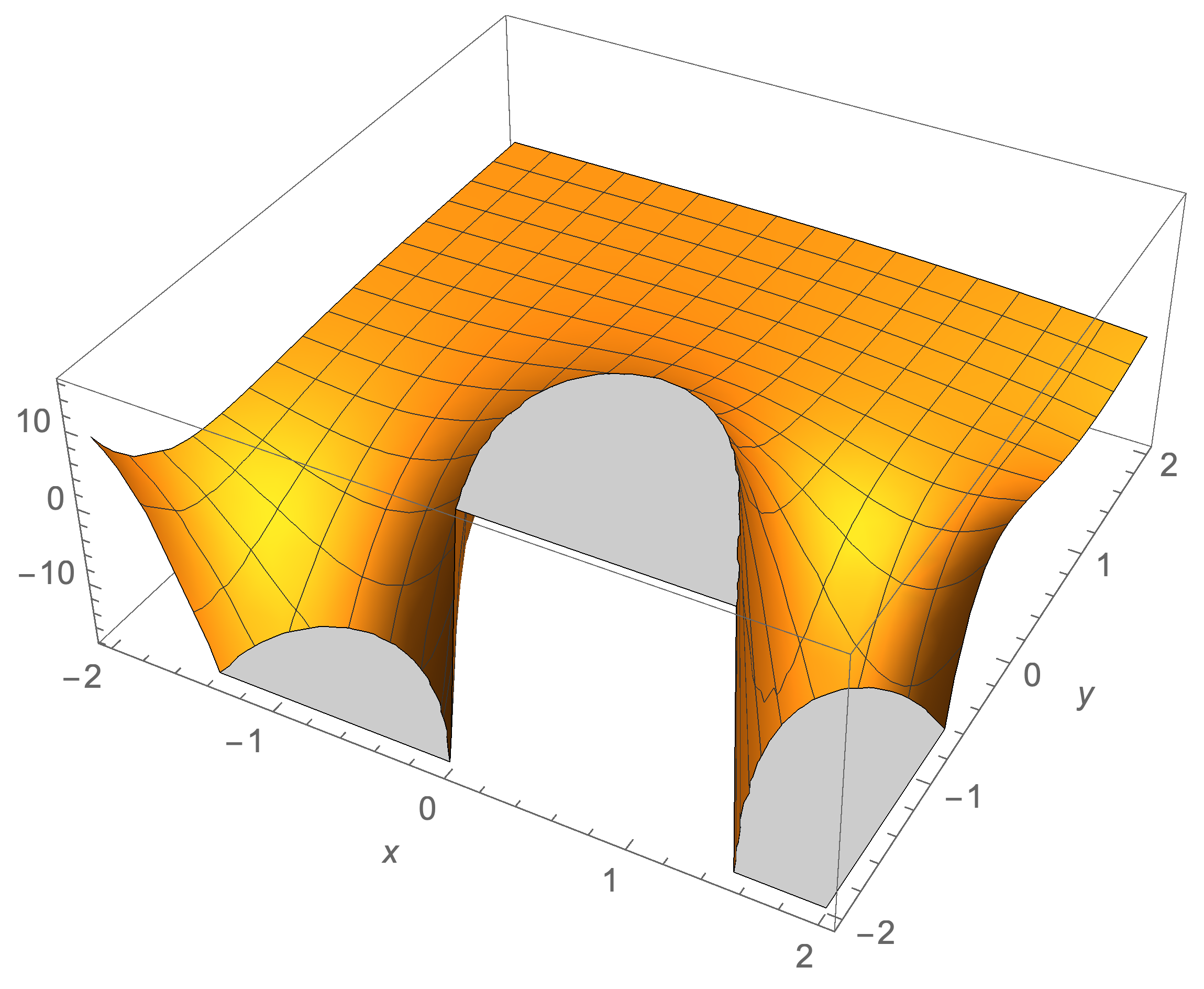
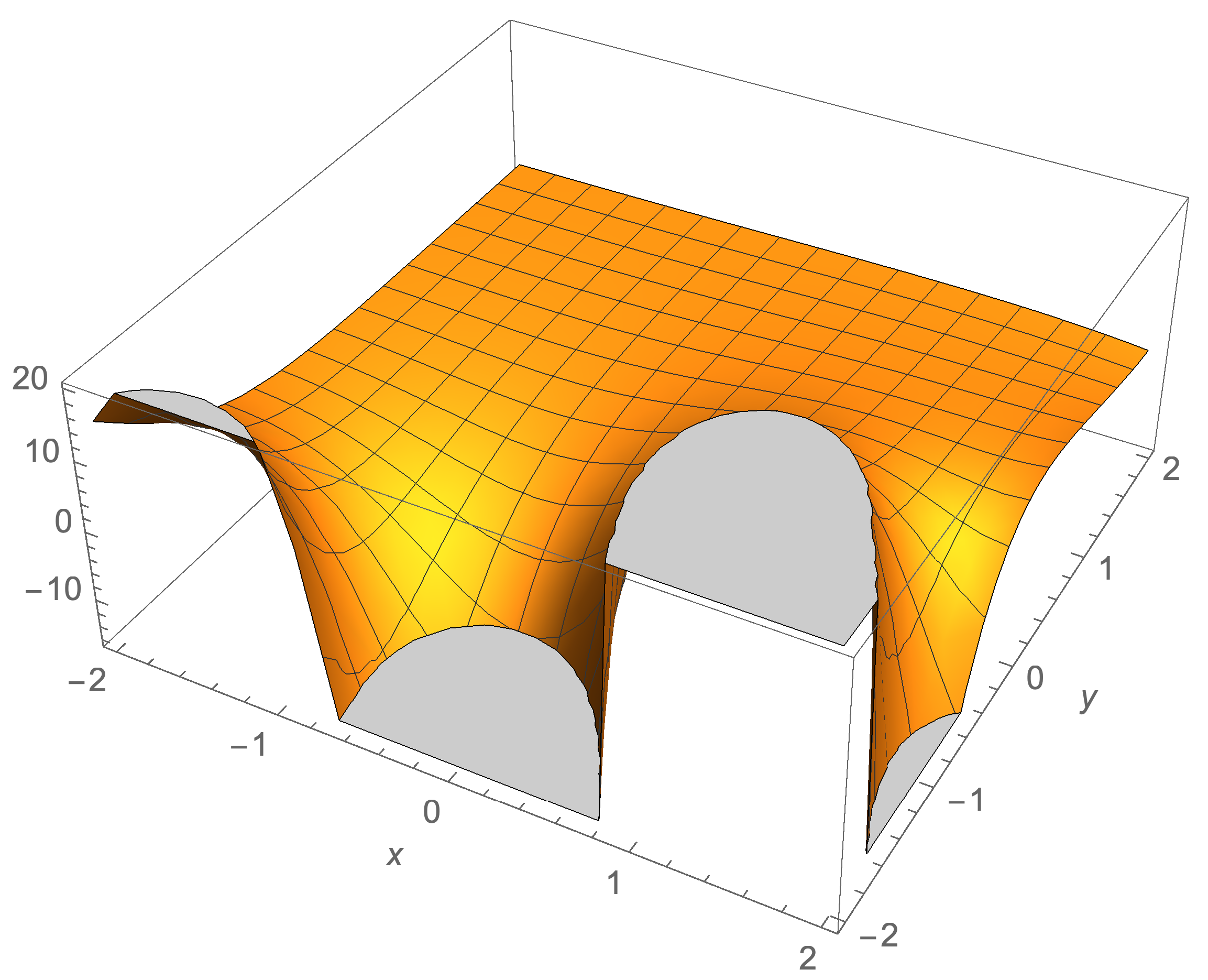
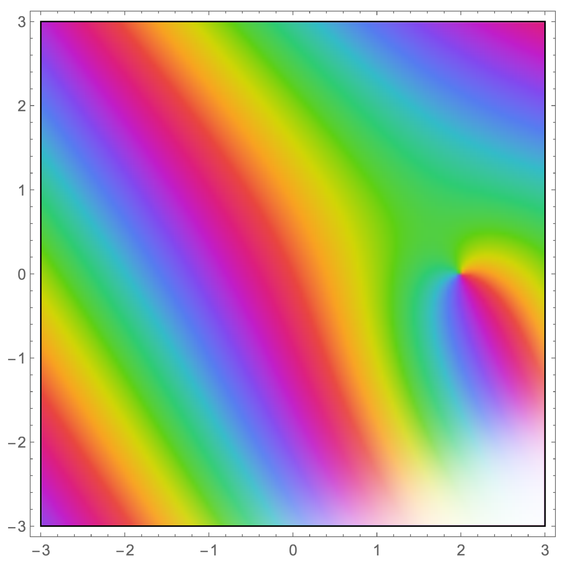
Plots of a Special Case Involving $\zeta \left(k\right)$

In this section, we evaluate the right-hand side of Equation (15) for complex values of the parameter k. The Figure 1, Figure 2 and Figure 3 are below:

7. Conclusions and Observation

In this paper, we have presented a novel method for deriving a new integral transform involving the product of the Struve and parabolic cylinder functions along with some interesting definite integrals using contour integration. We also derived an invariant index form of the quadruple integral. We observed that the single integral of the product of the Struve and parabolic cylinder functions is in terms of the gamma function, while the higher dimensional integrals of the product of these functions can be constant. We will be investigating this property in future work. The Figure 1, Figure 2, Figure 3, and results presented were numerically verified for real, imaginary, and complex values of the parameters in the integrals using Mathematica by Wolfram.

References

1. Watson, G.; Whittaker, N.; Taylor, E. A course of Modern Analysis, 3rd ed.; Cambridge Mathematical Library: Cambridge, UK, 1927; p. 353. [Google Scholar]
2. Mitra, S. On certain infinite integrals involving Struve functions and Parabolic cylinder functions. Proc. Edinb. Math. Soc. 1946, 7, 171–173. [Google Scholar] [CrossRef] [Green Version]
3. Reynolds, R.; Stauffer, A. A Method for Evaluating Definite Integrals in Terms of Special Functions with Examples. Int. Math. Forum 2020, 15, 235–244. [Google Scholar] [CrossRef]
4. Gradshteyn, I.S.; Ryzhik, I.M. Tables of Integrals, Series and Products, 6th ed.; Academic Press: Cambridge, MA, USA, 2000. [Google Scholar]
5. Brychkov, Y.A.; Marichev, O.I.; Savischenko, N.V. Handbook of Mellin Tranforms; CRC Press: Boca Raton, FL, USA, 2019; p. 149. [Google Scholar]
6. Harrison, M.; Waldron, P. Mathematics for Economics and Finance; Taylor & Francis: Abingdon, UK, 2011. [Google Scholar]
7. Olver, F.W.J.; Lozier, D.W.; Boisvert, R.F.; Clark, C.W. (Eds.) NIST Digital Library of Mathematical Functions; With 1 CD-ROM (Windows, Macintosh and UNIX). MR 2723248 (2012a:33001); U.S. Department of Commerce, National Institute of Standards and Technology: Washington, DC, USA; Cambridge University Press: Cambridge, UK, 2010. [Google Scholar]
8. Laurincikas, A.; Garunkstis, R. The Lerch Zeta-Function; Springer Science & Business Media: Berlin/Heidelberg, Germany, 2013. [Google Scholar]
9. Oldham, K.B.; Myland, J.C.; Spanier, J. An Atlas of Functions: With Equator, the Atlas Function Calculator, 2nd ed.; Springer: New York, NY, USA, 2009. [Google Scholar]
10. Lewin, L. Polylogarithms and Associated Functions; North-Holland Publishing Co.: New York, NY, USA, 1981. [Google Scholar]
11. Adamchik, V.S. Polygamma Functions of Negative Order. J. Comput. Appl. Math. 1999, 100, 191–199. [Google Scholar] [CrossRef] [Green Version]
Figure 1. Plot of real part of 2 2 k + 1 1 e i π k 2 π k + 3 2 ζ ( k ) .
Symmetry 14 00009 g001
Figure 2. Plot of imaginary part of 2 2 k + 1 1 e i π k 2 π k + 3 2 ζ ( k ) .
Symmetry 14 00009 g002
Figure 3. Plot of arg of 2 2 k + 1 1 e i π k 2 π k + 3 2 ζ ( k ) .
Symmetry 14 00009 g003
Publisher’s Note: MDPI stays neutral with regard to jurisdictional claims in published maps and institutional affiliations.