Abstract
Up until now, studies of Kauffman network stability have focused on the conditions resulting from the structure of the network. Negative feedbacks have been modeled as ice (nodes that do not change their state) in an ordered phase but this blocks the possibility of breaking out of the range of correct operation. This first, very simplified approximation leads to some incorrect conclusions, e.g., that life is on the edge of chaos. We develop a second approximation, which discovers half-chaos and shows its properties. In previous works, half-chaos has been confirmed in autonomous networks, but only using node function disturbance, which does not change the network structure. Now we examine half-chaos during network growth by adding and removing nodes as a disturbance in autonomous and open networks. In such evolutions controlled by a ‘small change’ of functioning after disturbance, the half-chaos is kept but spontaneous modularity emerges and blurs the picture. Half-chaos is a state to be expected in most of the real systems studied, therefore the determinants of the variability that maintains the half-chaos are particularly important in the application of complex network knowledge.
1. Introduction
1.1. For Mathematicians
This work is dedicated to mathematicians; however, there are no equations here. Therefore, it is an opportunity for specialists to be the first in this promising field, but it is not an easy task. We present experimental results from the simulation of a simple model that confirms the existence of half-chaos in growing autonomous and open Kauffman networks. The description is exact enough for computer scientists to repeat our results, so it should also be enough for mathematicians to understand their task. In the constant structure of large Kauffman networks, half-chaos has already been found and published [1]. The mathematical description should first be constructed for this simpler situation. Half-chaos, however, exists in finite discrete networks, but its existence in infinite and continuous space is doubtful. This is the reason the current chaos theory does not expect its existence. Building theories for finite and discrete networks is a great task for mathematicians. Our results indicate what should be noted in this theory and what assumptions are necessary for it.
1.2. Aims, Circumstances and Objectives
Half-chaos used in the title has already been introduced and described in articles [1,2,3] and documentation [4]. Preprint [5] should also be treated as playing a large role in these documentations in the first part (met8) of this article. All this research has common basic assumptions and variables that are repeated here for the necessary completeness of this article. They were based on Kauffman autonomous network simulations where only the functions of the nodes were disturbed while the network structure remained constant. The accumulation of such disturbances left in the network on the condition of ‘a small change’ in the functioning of the network (small damage) causes evolution of a half-chaotic system. A small change is well defined there. This condition works like the adaptation condition but is weaker, so evolution is not adaptive, only semi-adaptive. The results, in addition to previously known states of the networks-chaos and order, clearly indicated a new state called half-chaos.
Deterministic chaos and order are the properties of the functioning of a network-modeled system that determine its stability after a minor disturbance. Previous studies (e.g., [6,7,8,9,10,11,12,13,14,15,16,17]) have focused on the conditions of dynamics and stability resulting from the structure of the network, mainly the scope of the connectivity parameter K, which allowed one to predict whether a given network is chaotic or ordered. These predictions assumed full randomness of the network structure, usually including the functions and states of nodes.
Investigations described in [1,2,3,4,5] together with the actual article are the second stage of research in a topic of adaptive evolution of complex networks. They are based on a new, much stronger algorithm called ‘tmx’ (from maximal time t of damage watching). Earlier investigations [18,19,20,21,22,23,24,25,26] are based on a simplified algorithm called ‘rev-ann’ (reversed annealed—similar simplification to Derrida annealed approximation model, but here only damaged areas of the network were watched). Their aims were ‘structural tendencies’ for the description of classic ‘regularities of ontogeny evolution’. These earlier investigations are important bases for current ones, especially [26], which shows a base of s ≥ 2 and overlapping of left and right peaks when free inputs and outputs of the open system are assumed. Similarly, many used assumptions are described shortly, but their wider premises are not repeated, only linked to earlier papers, therefore all systems of shortcuts and terms are consequently kept. In the current article, continuing these investigations, we prove the hypothesis that half-chaos also occurs in autonomous and open growing networks, i.e., adding or removing nodes that change the structure. An important factor in such an evolution of a half-chaotic system is the spontaneous appearance of modules (i.e., classic modularity) in an initially randomly constructed network.
Grassi [27] presented a recent study regarding the applications of chaos in the real-world, including subjects such as distributed sensing, mobile robots, encryption, etc. Martínez-Giménez et al. [28] studied the subject of chaos on fuzzy dynamical systems. Wang and Robnik [29] treated the subject of multifractality of quantum chaos. Manera [30] presented a study on perspectives of chaos in environmental pathology.
The deviation from the randomness of the function was also noted as a factor shifting the chaos/order phase transition (the mean internal homogeneity P [9,31], ‘canalyzing’ [32]). ‘Ice’ was given as the primary property of a range of ordered systems. It consists of the lack of changes in the nodes’ states.
Kauffman [9] agreed that negative feedbacks are among the basic mechanisms that stabilize functioning. Their effect is to maintain an unchanged output state (more precisely, to maintain the output state in a narrow, safe range), which in the case of a simplified model based on Boolean signals comes down to a constant state of the node. Therefore, he believed that an ordered network with a strong predominance of ice (constant node states) models the network well stabilized by negative feedbacks. It can be understood that this is an accurate first approximation that roughly shows the properties of a stable complex network, but this approximation is still very simplified and describes many important aspects incorrectly, with oversimplification. First of all, it ignores the possibility of the negative feedback mechanism breaking out of the range of correct operation, which is the basis of most failures, and thus the main reason for leaving the system stability area. Of course, the path of successive approximations is the only way to more and more accurate descriptions and predictions, and the detection of half-chaos is the next step that corrects the basic shortcomings of the first approximation. Most systems built for a specific action (including living systems—the result of natural selection) lie in the half-chaos range, not ‘on the edge of chaos’, which radically increases the range of acceptable structure parameters. In particular, connectivity K (described widely later) is typically estimated out of range allowed by ‘life on the edge of chaos’ [13,33,34,35] but allowed in half-chaos.
It turns out that the structure is rather of secondary importance (all the studied network types—random Erdős-Rényi (1960) [36], ‘BA’, i.e., scale-free of Barabási, Albert, Jeong (1999) [37], single scale (Albert, Barabási 2002) [12] and others network types that show the presence of half-chaos—differ slightly in the degree of ordering), and the stability of functioning is mainly influenced by specific, holistic properties directly related to the functioning. These properties are not easy to describe, and typical statistics describing the system do not notice them. The mathematical description of half-chaos is a difficult challenge for mathematicians, even more so as the discrete and finite nature of the network is an important element here. Chaos theory based on Lyapunov exponents turns out to be too crude an approximation [1,2]. Such conclusions, even the direction of research, are absent in a wide range of investigations of chaos and complex networks (see books: [38,39,40,41,42]), but our simulation experiment proves it. Describing these experimental results in mathematical language will take a long time and require the hard work of mathematicians, and it is a next step that is not yet present in our work.
The overall picture of a half-chaotic system closely resembles that of an ordered system—usually ice with separate activity ‘lakes’ with properties similar to modules. However, they do not have to be modules in terms of the connection structure, although they do correlate in practice with such inhomogeneities. These are called ‘in-ice-modularity’. Altenberg [43] does not indicate such types of modularity and similar mechanisms.
The most important difference between the second approximation and the first approximation is the ability to exit relatively stable half-chaos through a minor modification that does not change typical structure statistics but does enter a normal state of chaos. At the same time, it is possible to maintain the state of half-chaos in evolution for a long time, leaving similarly minor disturbances that result in a ‘small change’ in the functioning of the system. A ‘small change’ is well defined in a natural way. A simple and easy to construct (with good random statistics) example of a half-chaotic system is a system with a point attractor. Such a system, despite ‘random (structural) statistics’, is not completely random, but the deviation from randomness is small. Its behavior, however, is radically different from that of fully random systems (even though the set of fully random systems contains a set of half-chaotic systems). The half-chaotic system reacts to a small disturbance in a chaotic manner and in an orderly manner with a similar participation, so it is at the same time partially ordered and chaotic, and it is not related to a place, e.g., a node, that has been disturbed.
The mechanism of half-chaos-preserving evolution is basically a Darwinian mechanism, except that the condition of only a small change with additional assumptions becomes a condition for adaptation. Adaptation is an adjustment to the imposed external conditions. Autonomous systems do not have such an ‘outside’. In the main work introducing half-chaos [1], only disturbances consisting of a small change in the functions of single nodes in three structural types of networks (scale-free, single scale, Erdős-Rényi) were investigated. It became a natural necessity to check that the half-chaos occurs regardless of the form of the disturbances, and here the basic candidates were structural disturbances consisting of a random addition or even removal of nodes. It still had to be checked on autonomous networks to limit the number of new factors. This paper first presents the results of such experiments. They confirm the generality and thus the importance of the half-chaos, but at the same time, new phenomena and problems arising from them appear. A significant obstacle to this research is the spontaneous modularity that appears in such an evolution, which strongly blurs the image. Furthermore, removing nodes destroys the clear structure emerging from the rule of node addition and generates ‘blind nodes’ (without outputs).
In order to reach the model in which adaptation may occur, it was necessary to study the occurrence of half-chaos in open systems, i.e., with input and output connections with the environment. This is the second important task undertaken in the research reported in this paper. The introduction of links to and from the environment, even at the beginning when input signals are constant, introduces new phenomena, limitations, and requirements to this research, which leads to the particularly great complexity of the studied phenomena. The main effect of these studies is that in open systems, there is also half-chaos. Half-chaos is therefore a state to be expected in most of the real systems studied. Therefore, knowledge of the determinants of the variability that maintain half-chaos is particularly important in the application of knowledge about complex systems.
1.3. Form of Results
The research showed clear conclusions, but the great complexity results in their simple, traditional presentation being hardly possible and completely inadequate. The form of most of the results are simulation runs visualized in a complex way on screen pixels. These are qualitatively assessed results, of a statistical nature, but are strongly dependent on the specific properties of a given unit network, the simulation of which usually takes several hours. The wealth of phenomena noted is a good investigation for many future large works. Their more advanced analysis would require simulation times many times larger. A large range of network parameters was tested, because each choice of these parameters is arbitrary, and more general sentences require testing many variants, i.e., many networks with different parameters were simulated. Most of the specific sets of these parameters were tested on 10 or 15 different networks, and due to the low sensitivity to one of the main parameters, it was possible to combine the results into 25 networks with practically the same parameters. Similar parameters gave similar results, which significantly increased their credibility.
Undoubtedly, this direction of research should be continued, but it must have many stages and many threads. The presented results are a good recognition of this area of knowledge that explain many phenomena observed in complex, evolving systems. Such properties are commonly expected to be described in the language of mathematics, that is, using equations. Currently, it is a long process to do so, using accepted scientific tools only, and simulations of models increasingly close to natural living or man-made systems are at researchers’ disposal. The models used in this work and earlier works are simple, not limited by any additional assumptions; they are only Kauffman networks, autonomous or open. Further models will apply additional assumptions and will undoubtedly become increasingly complex. Complex evolving systems have many applications, such as self-organizing overlapping community detection [44] just to mention an example.
1.4. Structure of Our Article
The first sub-chapter of ch.1-Introduction has already described aims, circumstances, and objectives, and herein, brief a structure is clarified. The main theme—half-chaos—is studied in growing networks of two categories: Autonomous (ch.3, symbol of investigation stage and method—met8) and open (ch.4, symbol—met9). Before them (in ch.2), common assumptions, terms, and variables of the model and algorithm are described, including repetition of earlier works.
For autonomous networks (ch.3), three themes were studied: The main, an evolutionary stability of half-chaos, as well as a tendency of conservativeness of older nodes as an example of structural tendencies, and the effects of modularity that generated problems in investigations of the main theme but also are important elements in the stability problem of complex systems. For the main aims of this work, only the first theme is important, and the next two may be skipped depending on the reader’s interest. More details can be found in [5].
In the open network investigation (ch.4), only the main problem of evolutionary stability of half-chaos was studied but growing open complex networks especially have many aspects and issues of potentially very high importance and scientific impact. It is more important that such problems exist, followed by a deep understanding of data and details. However, how deep an understanding is already desired depends on the particular reader. This required a new, extended program for the simulation and examination of many variants.
Conclusions of our investigations (ch.5) are positive: The hypothesis that half-chaos exists and maintains evolutionary stability in increasingly complex autonomous and open networks is proved, but half-chaos has a competitor in the form of growing modules, which, in the current model, in some circumstances can destroy it.
2. Model and Algorithm
2.1. Main Terms and Variables
A network consists of N nodes. A node receives signals from K inputs, converts them uniquely using its function to the output signal called the state of the node, and then sends it to other nodes by k output links. K and k have long been commonly used symbols. The state of the network consists of all N nodes states. The calculation of node function takes a time step. The signal typically had s = 2 (logical) states (variants), and we use s ≥ 2 of equally probable variants for reasons described in [26] (ch.2), see also [1] (ch.2.2). For logical cases (s = 2), with full randomness of connections, functions, and initial states of each node, such networks were called Random Boolean Networks (RBN).
RBN was limited to the Erdős-Rényi random networks type. At the time of the emergence of the discipline ‘complex networks’ between 1969 and 1999, it was practically the only network investigated in many significant publications and the basis for the Gene Regulatory Network (GRN) model (e.g., [6,7,8,9,10,45,46,47,48]). In 1999 [37], Barabási, Albert, and Jeong discovered that in reality, most networks follow a scale-free networks structure; then a variety of architectures began to be studied (e.g., [14,32,34,49,50,51,52]). Serra, Villani, and Agostini [53] proposed to rename the old Classic RBN to CRBN, and to use SFRBN for the Scale-Free Random Boolean Network. For comparison, Iguchi [54] used ‘directed Exponential-Fluctuation networks EFRBN’ known also as a ‘single scale’ network [12] where a new node links to a node in the current network with equal probability. We denote it as ‘ss’ [20,26] (ch.1.3). In the investigations of half-chaos, the er [36] network was, until now, the only one with blind nodes (nodes without outputs, with k = 0); however, the er network cannot be used in our investigation of growing networks, because it does not have the rule of growth (adding new nodes to the already existing network). Until the discovery [37] of the importance of scale-free networks (sf), RBN was synonymous with the Erdős-Rényi network (er). These two network types differ in structure. In our work, the deviation from full randomness is made by assuming a point attractor (the next network state is the same). This assumption, like the states of chaos/order and half-chaos, concerns functioning but not structure.
The states of nodes from the discrete time t are input signals—arguments of the function of other nodes—and the results of these functions are node states at the next moment (t + 1). This is synchronous computing. Variable t is the number of time steps from a disturbance initiation. The disturbance can take many forms. Here we apply the addition or removal a node, while in earlier work [1], a permanent ‘point’ change in the value of the function of the node for its input state was used at time t = 0. The parameter tmx—the maximum number of calculated time steps—is chosen arbitrarily tmx = 1000 based on previous works [1,4].
Our networks are deterministic—in an autonomous system, as well as in an open system with the same input signals, determining the states and functions of all nodes and the connections between nodes uniquely determines the trajectory—consecutive states of the whole network. We simulated the process of transformation of the disturbed system on the section tmx, then we compared the resulting state of the system with the undisturbed system.
The size of the change in network function at time t after a disturbance is measured by the number A (from Avalanche [47]) of the nodes, which have a different state in the undisturbed network. The value d = A/N is called damage. The distribution of damage size at time tmx as P(d) or P(A) is an especially important result. In chaotic finite discrete networks, damage grows up to the ‘Derrida equilibrium level’ dmx—given by the Derrida annealed approximation model [6,7], see also for widening on s > 2 in [26], or [1] (Figure 1). There have been attempts to increase the number of signal variants (e.g., [48], but they were not variants with equal probability.
The term ‘chaos’ is well defined in infinite and continuous space by Lyapunov exponents; however, it is also used by many researchers for finite and discrete networks. The main characteristic of the chaotic behavior of dynamic systems is high sensitivity to initial conditions, leading to maximally different effects for very similar initial conditions. The distribution P(d) of the damage size is the experimental base to classify a particular system of a network as chaotic or ordered, using levels of the damage equilibrium calculated from Derrida’s annealed approximation.
The Lyapunov exponent corresponds to the so-called ‘Derrida exponent’ [47] for finite discrete networks, or the “coefficient of damage propagation” w = <k>(s − 1)/s described in [26] (Section 2.2.1) and earlier defined in [18]. It can be treated as a damage multiplication coefficient on one node if only one input signal is changed. However, while it is statistically correct for a fully random network, our networks are not fully random.
Fully random networks can be either ordered or chaotic with narrow-phase transitions between order and chaos. The space of parameters near this phase transition is called the ‘edge of chaos’, and there Kauffman places life; however, now life should be shifted to the half-chaos of not fully random networks [1].
2.2. Half-Chaos
Half-chaos is a third state of the system in addition to chaos and order, but for it to be true, the system cannot be fully random. Parameters of the half-chaotic system make the random system strongly chaotic; however, small disturbances give an ordered reaction (small damage) with a similar probability to a chaotic reaction (near the Derrida equilibrium dmx). We call such parameters “chaotic”. For real systems, parameters are usually estimated in the range of chaotic parameters; however, behaviors of these systems are typically different than chaos. This behavior of the half-chaotic system turns out to be inconsistent with predictions based on its parameters (for a fully random system). Acceptance of the initiation changes that give ordered reactions leaves the half-chaotic state, allowing for a long evolution of the slowly changing system (it is the evolutionary stability of half-chaos, wherein the system retains identity), but acceptance of one change that gives a chaotic reaction leads to practically irreversible entry into normal chaos (the system works completely different, and ceases to be itself).
The distribution P(d) of damage size [9] or P(A) “size distribution of avalanches” in [34] is then the main feature observed in experiments and expected by the theory that may be compared. For a chaotic network, the P(d) contains one peak near dmx, and for ordered, one peak near d = 0. If there are both peaks in the distribution for one particular network, then it is neither a chaotic nor ordered network, and it may be half-chaotic. Such a picture of two similar peaks was expected by Gecow in [20] using the simplified algorithm ‘rev-ann’ [21,22]. Between peaks, there is a gap, where no cases happen. This gap defines ‘small change’ (small damage) in a natural way, which is needed for stabilizing half-chaos during evolution. To decide if this damage is small, a particular threshold of damage size is needed; it may be in any place of the gap, and for experiments it must be defined arbitrarily, but the gap is natural. However, the gap may be blurred by other phenomena, so defining the threshold may be not clear.
The constraints forming the half-chaotic system are small, which means that there are many such systems, though undoubtedly significantly less than fully random. The main, easiest method to obtain a half-chaotic network is to start from a ‘point attractor system’ (PAS). To obtain PAS, just after the fully random generation of networks (functions, initial states, and connections of nodes), it is sufficient to change each node function for the current input state to the current node state. For the remaining states of the input, the functions stay unchanged, but after such operation, functions remain random (when only a set of functions is considered). The point attractor system in Kauffman terms is a completely frozen system—there is only “ice” (nothing changes). The predominance of the ice is a spontaneous property of ordered systems. Damage after small disturbance of a frozen system is small and creates “a small lake of activity in the ice” (Originally [8]: “unfrozen islands”). This is the feature of the ‘liquid’ area of parameter space near the phase transition of random systems, where Kauffman sees life; however, such a system ceases to be a PAS.
The PAS has an extremely short attractor with a length of 1 time step. Attractor is a cyclic trajectory of system states; a number of time-steps until meeting the same network state is its length. It was checked [1] that for half-chaos, it is enough that the attractor is short enough. However, starting from PAS, the left peak is more suitable for the modeling shape than starting from a forced short attractor, but is greater than 1. It turns out that in the case of starting from a short attractor, there is no ice in the network, but when starting from PAS, the ice remains long during evolution and ‘small lakes of activity’ create ‘in-ice-modules’, where local attractors are typically small. In the network, there are a few such in-ice-modules simultaneously, and their local attractors assembled into a global one may make it even larger, but the network stays half-chaotic.
The main result, however, is a “degree of order” q—a fraction of damage after small perturbations, which build the left peak of P(d). This represents the probability of acceptance (lack of elimination) of changes in the modeled evolution. Such damage fits into the range of the “small change” of the functioning while it is measured at the time tmx. It is summarized in Figure 1b. A sufficient size of q is the base in which we found half-chaos in the range of chaotic parameters.
2.3. Network Types
Two basic and two secondary types of networks are considered; however, for a special reason, one additional basic and secondary network is included. The basic network types grow using only the random addition of nodes, and they are (for an outgoing link only) sf (scale-free [37]) and ss (single-scale [12]). They differ in the rules of their creation and distributions of k (number of output links). We fix K— the number of input links for all nodes of a particular network. The secondary, albeit our main object of interest, networks sh and si are respectively sf and ss with the removal of nodes, but these removals destroy the typical distribution P(k) for basic types and creates some nodes without outputs (called ‘blind node’, k = 0). In the case of the ss network, the addition rule links a new node with other nodes present in the network with equal probability, and then the blind node can recover the output, but for the network sf, a new node is connected to indicate the node proportionally to its k, therefore for type sh, we use addition proportionally to k + 1 to allow for a such blind node to come back into play. Additional network types are ak (only additions) and al (additions and removals of nodes), and their rule is K = k and are both fixed. For rules of the addition and removal of nodes, see in Appendix A Figure A1. They are described (mainly in [26] (Figure 2), earlier in [25] (Figure 1), [23] (Figure 4)) in-depth in [26] (Chapter 1.3.3, 1.3.4, and in Figure 2).
The second letter of these shortcuts indicates the network type (i.e., for sf, ss, sh, si, ak, al, we use f, s, h, i, k, l, respectively. In earlier works [1,26], only one letter was used on figures with two letters in the text, while in our work, we use only a one-letter name, but the two-letter names are shown above for easier connection to earlier works. Such a connection is important, because some themes described earlier needed to understand current problems cannot be repeated here). In similar investigations [1,4,5] and earlier works on structural tendencies with the rev-ann (reversed-annealed) algorithm [21,22], more network types are considered. Up until the work in [37], practically only classic Erdős-Rényi [36] “random” networks are investigated, for s = 2 known as RBN. They contain blind nodes. In [1], the Erdős-Rényi random networks were the only type with blind nodes; however, they cannot be used in our investigations because they do not have the rule of growth.
Parameters vector: (network type,s,K) is the main variable in the simulations (type ϵ {f, s, h, i}, s ϵ {2, 4, 8, 16, 64}, K ϵ {2, 3, 4}).
2.4. Earlier and New Stages of Investigation
The half-chaos was detected in simulations conducted by Gecow described in [1] especially in so-called met4–7. The acronym ‘met’ is from ‘method’. In [1] and its documentations [4], met4 is an investigation only of point-attractor networks without evolution, met5 is the investigation of its evolution, met6 is the starting evolution from the short attractor, and met7 –is the starting evolution from an in-ice modularity. In these simulations, the network structure was a fixed-node number N, and the node’s connections are stable during evolution. Changes initializing damage are limited to the permanent point change of one function value for one node function and its one initial input state. These were very small disturbances. Such changes were accumulated as evolutionary changes when the resulting damage was small. Evolution takes 20 stages, and in each stage, all available initializing changes were used (skipping reverse changes in a few consecutive stages). Such an algorithm gave the conclusion that half-chaos exists, but the question remains: Does it also exist in larger sets of the types of permanent changes initializing damage?
The current investigation, as a continuation of earlier ones, introduces met8 for autonomous growing networks and met9 for open growing networks. All of these are investigations of the existence conditions of half-chaos. The addition of nodes is the most interesting type of such evolutionary changes, followed by the removal of nodes. Here, we check the evolution of initially half-chaotic (we start from PAS) growing networks. Of course, for networks growing under these conditions, the structure ceases to be constant and random.
Our investigations are a continuation of a large project started in [1], therefore consecutive stages are called met8 (method 8) and met9. In the first stage (met8) of our research, autonomous networks are tested, like in Kauffman investigations and in [1]. Open networks are tested in the second stage, met9.
3. Growth of Autonomous Networks (met8)
3.1. Algorithm and Problems
3.1.1. Algorithm
At the initial stage of growth, a network of 50 nodes is built according to the rule of a given type. Then, the initial states and functions are drawn—we obtain a fully random network. Now the functions for the initial state of the input of each node are changed to give their initial state (i.e., the states of nodes from the moment t = 0 and t = 1 are to be the same). This creates a PAS. The addition of nodes is further drawn, and for h, i, which are respectively f and s for addition, the removal of nodes is also drawn, of which the share is 30%. The networks of s,K = 4,3 are tested. As in [1], the shift by t = 50 of the trajectory beginning after the accumulation is used.
Changes that give damage less than the threshold (it will be later described), denoted as ‘small damage’, are ‘accepted’ (denoted as ‘a’, e.g in P(a|M)), but not all accepted changes are accumulated as evolutionary changes, which means they are left in the network. For statistics, the number of accepted changes is collected, but only those accumulated in the network remain. This difference is scheduled for simulation optimization.
Up until the attractor of the growing network achieves a length of at least 7, the attractor cannot decrease (even acceptable changes are not accumulated), i.e., it still cannot fall below 7, but when this condition blocks the accumulation for too long (more than 60 times), the currently proposed attractor of less than 7 is allowed and again it cannot decrease until it not exceeds 7.
Further growth of the network is divided into 10 passes, in which the network increases by the next 50 nodes, so that it ends on a value of N = 550 nodes. These are passes 2-11 indicated in the figures of A(t) or d(t) tracked dynamically and shown in Figure 4 called ‘crocodiles’, but to analyze the collected data, it turned out that these passes are too small (apart from the tendency and modularity test). In such an analysis presented further, the graphs use stages M1–5, created by summing up two successive passes of the tracked evolution, so that M1 is pass2 + pass3.
During the preliminary simulations, the threshold was set at d = 0.4 (which means 0.4 of current N); however, the problem of filling the interval between left and right peaks in the damage distribution discussed in Figure 1 led to the selection in the main simulation of the threshold d = 0.2 and the comparison of results for the threshold 0.5.
3.1.2. Problem of Threshold Level Definition due to Oscillation Inside Modules
In the studies described in [1], which show half-chaos (our investigations are a continuation of them), the process that crossed the threshold almost never returned to under the threshold. This allowed for optimization—an interruption of the counting of those processes that were above the threshold more than 70 steps from the first cross. At that time, they could decrease below the threshold and stay there, but this never happened, and the size of the fluctuation was usually so small that they were far from the threshold. This was due to the small size of the resulting in-ice-modules. Classic modules were so weak that the effect of them was not visible. In our study, however, there are relatively frequent cases of larger in-ice-modules or especially strong classic modules or probably other similar phenomena (we will call all of them the ‘module’). The fluctuation range after crossing the threshold is so large that the threshold level is often crossed and the chance that, at tmx, A1 (the temporary value A—the number of nodes with a state different from the pattern) will be just below the threshold is considerable. Such cases should be (statistically) eliminated by the criterion A3, which is the average of A1 on the last stretch of 50 counting steps.
It turns out, despite A3 being below the threshold, the frequent presence of the process above the threshold allows one to create a pattern after the accumulation and shift, which with a much higher probability also leads to large modules, and even chaotic collapse (more in [5]). The observation of these large modules strongly suggests that they arise under the influence of evolutionary pressure resulting from the condition of small change. Such a hypothesis is examined in chapter 3.4 and partially turns out to be correct.
For the purity and simplicity of acceptance and accumulation criteria, a rule has been introduced that the process that has returned under the threshold is still counted, and its counting ceases after 70 steps since the last transition over the threshold. This caused a large part of such processes, even with A3 over the threshold, to be counted for a long time, even to the end (Figure 4c,d).
The presence of processes oscillating around the threshold causes a “backfilling” gap in the distribution P(A3) (the form of the distribution P(d)—of damage size, Figure 1). The gap between the left and right peaks has significant interpretive meaning in the half-chaos concept. It allows for the natural criterion of elimination and maintenance of half-chaos—the evolutionary stability of half-chaos observed in [1]. Backfilling this gap caused the threshold position to became meaningful and cease to be well-defined, and the responsibility fell on its arbitrary choice. Therefore, instead of the 0.4 N threshold (d = 0.4) used in the initial simulations, the thresholds 0.2 N and 0.5 N (Figures 1a, 2, and 3a) were used to compare the effect of this arbitrary choice. It can be noted, based on these figures, that the low threshold allows for smaller backfilling of gaps between the peaks, but it is clearly arbitrary, even on the fall of the left peak. Moving the threshold according to this diagnosis close to the minimum gives a different image, in which additional peaks are created in this area in the h and i networks. They are small compared to the right and left peaks, but several times greater than for the smaller threshold. The minimum separates into two complicated interpretations, and for growing networks, the evolutionary stability of half-chaos and the criterion of identity are slightly weaker. The size of the initiating change, which is the addition or removal of the node, may be a cause—it is not a small change, and it cannot be reduced. The threshold of 0.5 N was used to study the effects of modularity, because it gave a wider range for testing, not intensely colliding with the threshold.
Based on these investigations, the problem is clarified: Disturbance in not a very small module under the threshold may cause a ‘large’ change of module function, but only inside this module. In a large network, the threshold allows for so large a module under the threshold, that we can say it falls into chaos and reaches Derrida equilibrium without a short local attractor. It is not under the control of elimination, which concerns the whole network and its threshold. In effect, the changes (the addition and removal of node) are accepted and accumulate and the module grows, being proportionally faster than the whole network. Therefore, such a module reaches a threshold and ceases this problem. We will discuss it more deeply later, but it is a new phenomenon that does not exist in [1,2,3,4], and is the main competing factor of half-chaos.
3.2. Results in Half-Chaos Aspect
In the first subsection, we repeat the definitions of the observed variables from [1,2,3,4,5] and indicate the main figures in the range of Figures 1–4, where they are shown as measured during the simulation. These figures, as the results of our experiments, are included in the next two subsections, along with extensive descriptions.
3.2.1. Distributions P(d), q, P(k) and Ice
The basic simulation series contains 600 networks of type h, i, f, s, with s,K = 4,3.
Evolution is observed during stages M1–M5, each consisting of 2 passes of 2-11 visible in crocodiles, which increase N by 50, so during M1 (it is pass2 + pass3) the network grows by 100 nodes. The principal results are:
P(d|type)—damage size distribution (Figure 1a) for the stabilized stages M2 to M5, for a particular type and threshold 0.2 N or 0.5 N. It is measured by the value A3 as P(A3|type) for comparison and uniformity with the results of previous works; however, here N grows and A3 is substituted by d = A3/N. The initial stage M1 turns out to be slightly different, which can be clearly seen in Figure 2, and further stages are already similar and can be combined.
q(type)—degree of order (Figure 1b) is calculated from the above P(d|type) based on the threshold d = 0.2. For the h and i networks, it contains a piece resulting from k = 0. The degree of order is the basic result showing a significant presence of order, which mainly distinguishes half-chaos from chaos.
q(M)—degree of stabilization of evolution (Figure 2a) (see for comparison in [1] (Figure 8a) allows one to state that the evolution was carried out for long enough.
q(t)—degree of stabilization of the process after the disturbance (Figure 1c and crocodiles in Figure 4) is the basis for recognizing tmx as sufficient (see for comparison in [1] (Figure 10c). This problem was also examined (as in [1] (Figure 8b)) through the range of t of the explosion to chaos—the average t for the five latest explosions (Figure 2b). Here, similarly to in the M2–5 range, this average time practically does not grow.
P(ice size|type) (Figure 3), <ice>(M|type), (Figure 2c)—ice distributions. This is the main argument for the similarity of the mechanism studied in met5 and 7 described in [1], called in-ice-modularity. Current part of the investigation concerning autonomous networks is announced as met8. Only for the s network, the average ice in the studied range of evolution is clearly declining, which may raise anxiety about whether this decrease will stop at the level that still entitled the mechanism to in-ice-modularity and evolutionary stability of the so-obtained half-chaos; it should be noted that the scale in Figure 2c begins above the middle of the range.
P(k|type)—node degree distributions (Figure 3b) first of all justifies the use of the names ‘scale-free’ and ‘single-scale’ of the types f and s and indicates the deviations from f and s, which the removal of nodes in types h and i introduces.
3.2.2. Measured Results
Measured statistics are shown in Figure 1, Figure 2 and Figure 3. These figures need a deep description in the legend to be comprehensible, but such a description is sufficient and needs not to be repeated in the text of the chapter.
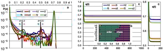
Figure 1.
The main results of checking half-chaos existence in the autonomous growing networks. Specifically for half-chaos, two peaks of P(d) with a deep gap between exist, also a great part q of ordered reaction on disturbance despite s = 4 and K = 3. Fraction q of ordered reaction (below threshold) stabilizes during time of calculation after disturbance on high level. (a) Damage size distribution P(d) during growth from N = 50 to N = 550. Damage is always scaled to current N. Two series—for threshold = 0.2 and 0.5 current N marked after network type by digit 2 or 5. For each network type of h, i, f, s, 600 networks’ growth is simulated. Note that it is logarithmic scale, and the gap between peaks, however not empty, is deep, and on linear scale, capacity of gap is invisible. The capacity of gap will be later discussed; it is created by modules, which for particular networks give much clearer additional peaks, but in different places. These additional peaks appear most intensively for the i and h networks in which the nodes are removed; much weaker in f and s, where there is no removal. They are intensified by the increase in the threshold level. (b) Share of q—order and 1-q chaos is included in the empty area of q(t) plot (c). Order i.e., q, is a capacity of left peak from threshold to the left, then chaos is the capacity of right peak. More precisely, it is the number of reactions on additions or removals of node, which fall to areas of small or large damage. In the case of network, h and i P(k = 0) is 0.08 and 0.034, respectively, which is marked in yellow as the order of other origin. As can be seen, fraction of ordered cases is typically large despite s = 4 and K = 3, which are ‘chaotic parameters’ (cause chaos in fully random network). (c) Level of q during calculation of networks function, i.e., q(t), after addition or removal of node up to tmx = 1000. For chaotic network, it falls down monotonically, and for t much less than tmx, all checking processes cross the threshold and become ‘chaotic’. For half-chaotic networks, a large fraction of these processes reaches second round of attractors still below threshold, and after this point, they stay on stable level of q. Here, these levels reach stability before t = 100, therefore tmx is taken as not too small. On the right, the crucial period is repeated more exactly.

Figure 2.
Additional important results confirming the stable presence of half-chaos. Important parameters in consecutive stages of growth. Each stage M network grows by 100 more nodes. The growth of autonomous networks starts from 50-node network built as point attractor system; the next networks grow under conditions up to 550 and that period is divided by stages M. (a) Stable level of q at high level. The selection of the threshold practically did not affect the distribution of q(M), and the presence of removing in the h and i networks also has a slight influence. (b) Average time of 5 the latest explosion to chaos. For chaotic networks, explosions happen until practically all processes achieve Derrida equilibrium over threshold. In our investigated case, explosions stop long before tmx. The 5 latest explosions expressly depend on the initial stages M1 on the threshold height for the networks h, i, f but not for s—a low threshold increases the chance of passing through it, but mainly at the beginning of the evolution. The descriptions in (a–d) have the same colors. (c) Average share of iced nodes is given as the share of nodes not changing their state among all nodes of the network. Here too, the choice of the threshold has negligible impact. Presence of ice is not an obligatory feature of half-chaotic networks, but it causes a more interesting type of half-chaos, more adequate for modeling the shape of left peak. Presence of ice in such a level indicates similarity of mechanisms as those observed in [1]. (d) Average attractor. Short attractor is the main cause of half-chaos. As was shown in [1], it is enough to create half-chaos; however, if there is too little ice, then shape of left peak is not usable for modeling.

Figure 3.
Distributions of ice size and of ‘node degree’ k-number of output links. (a) Distributions of ice size. Ice does not grow; however, as was shown in Figure 2c, it does not disappear as it does after reaching chaos. (b) P(k) is the main feature distinguishing scale free f and single scale s networks. For f, it should be a straight line in log-log diagram, for s in log diagram. The rule of node removal destroys these shapes for h and i network types, but it is not a very hard change.
3.2.3. Observations on Crocodiles
Much information about the investigated processes can be obtained from their dynamical view shown on screen in pixels during the simulation. However, such saved static pictures called ‘crocodiles’ also show important knowledge that is hard to describe in another way. We have included a few ‘crocodiles’ below as sub-figures in Figure 4 with common descriptions placed for convenience before the pictures.


Figure 4.
Examples of ‘crocodiles’ and their main elements. In the rectangle is runs A1(t) (black). After moving into chaos (above the threshold marked in red on the left, here some examples are from the initial simulations where the threshold = 0.4 N, but for the main simulation the threshold = 0.2 N and additional = 0.5 N), only 70 counted steps of time t are marked (horizontal axis, 1 pixel = 1 step t) but if at that time the process returned under the threshold, then it was counted on. Process of network functioning is counted up to tmx = 1000. The scale on the left refers to the end of the depicted pass, which starts from N-50. The A1(t) values are scaled: A1/Ncurrent * Ntermin. The red line is q(t) summarizing the pass in scale q = 1 for N. Similarly, the blue line indicates the share A1 = 0. The frequency of use A1 (below the threshold) on the right side of the rectangle is marked in beetroot color (see b). Above the black rectangle of A1(t), from the left, consecutive attractors are given numerically. Directly above the rectangle’s frame, the occurrence of the tmx state in the initial pattern is marked in green, indicating its attractor. Under the rectangle, diverse information can be found, such as number of calculated network treated as it’s individual ‘first’ name with type, s, K treated as it’s ‘family name’, pass number. The remaining data are not interesting here, and many other data are described and shown in [5]. Shown here, crocodiles should be watched on a screen in large zoom (pixel to pixel). (a) Typical view of crocodile: pass = 10 of 28-th network i, s,K = 4,3. It is a clearly half-chaotic case. (b) Less typical network cases h 4,3 (from initial series of simulations) in which there is quite a high additional ‘Derrida level’ suggesting the presence of a large in-ice-module or module. There are many different attractors, with a large spread, testifying to the complexity of the phenomena that took place here. Nevertheless, q(t) remains at a high level, which indicates the evolutionary stability of the half-chaos occurring here. Similar cases occur sporadically, and it is rather the property of a given network, because the images in other passes of the same network also show a similar character (see (c,d)). (c) Specific example 84 i 4,3 from the series with a particularly high 0.5N threshold. The module grows faster than the threshold, but after passing it over the threshold, the network regains stability (q level in red). Such a high level of Derrida balance indicates the size of the module, while the high level of q(t) indicates that the disturbances within this module can be accumulated. The subsequent attractors are shown in the whole range only for pass 3 (large number below), (900—the attractor was not detected). Such cases were the reason for undertaking the search for classical modularity in ch.3.4, where they were analyzed in the ‘great’ group. Modularity has indeed been found and the black belts observed here are Derrida equilibrium levels in local clusters of a module nature. This does not mean a change of the in-ice-modularity mechanism to modularity, since the ‘rest’ is ice, so both mechanisms work simultaneously in the same direction. There is another crocodile (140 s) of this type analyzed deeper in d. (d) Crocodile of s140 as an example for the ‘great’ set. Here in a fairly uniform section of the A1(t) of crocodile for pass 11 (last), the initial sections for passes 9, 7, and 4 are pasted, and the end again belongs to pass 11. In these crocodiles, the expected level of Derrida balance for local clusters designated in a given pass is marked in green. See Table 1 below for more information.
3.3. Tendency of Conservativeness of Older Nodes
The structural tendencies are statistical effects in the structure of complex processes, especially of living entities, resulting from the condition of elimination. They correspond to old, challenged regularities of ontogeny evolution. Tendencies have already been defined and described in [19,20,23], where it is the difference between a given random distribution and the distribution modified by the adaptation condition. Here, the equivalent of the condition of adaptation is a weaker acceptance condition based only on not exceeding the threshold of great change, but the modifying factor is the condition of accumulation, slightly stronger than acceptance (attractors larger than 6 to increase the strength of persuading the obtained results), because it maintains the particular, studied specificity of the system state called half-chaos (although acceptance is enough). In general, any statistical differences in nodal properties resulting from the evolution that maintains half-chaos (controlled by a small change) are tendencies. For example, the tendencies are the persistence of half-chaos and the persistence of a high level of ice after the start from the point attractor, which disappear immediately after allowing the accumulation of random changes.
It can be supposed that nodes, which are already in the network for a long time and have not been removed yet (in networks h, i, l), are actually more difficult to remove because of their environment (because of the importance of nodes connected to this node). Network type l is special, as it has k = K, therefore it is especially useful for this experiment (more about results for this and other types of networks can be found in [5]). The environment changes, and perhaps after some time from an ineffective removal attempt, lets it be removed. In cases of network h and i, a separate aspect is the gradual addition of outputs to nodes during evolution, which makes removal more difficult, so only the l network is suitable for easily checking this hypothesis. Therefore, an additional measurement of the probability of accepting the removals was made depending on the sequence of connection of a given node to the network. There was no recorded time of residence of the nodes in the network, and it was enough to divide the current set of nodes in the order of connection (which was already ready) for the consecutive 50-element sets. For h, i, l measurements during the last pass, f, s was used during an additional attempt to remove the nodes after reaching N = 550, without accumulation (Figure 5).

Figure 5.
Tendency of conservation of old nodes. Horizontal axis H-intervals of the sequence of the connection of the nodes corresponding to the “depth of history” and the “age” of the node. The 50 youngest among those currently presented, joined in the last order, constitute the range 0–50, and the oldest 50 among the currently presented range of 500–550. In the picture, networks h and i with thresholds 0.5 N and with 0.2 N have such similar P(a|H) values that they are summarized and shown as one line. Here, additional network type l is shown because it gives an especially important result. ‘l3′ is ‘l’ calculated with the threshold 0.2 N (l was not calculated with 0.5 N); however; in the wider report of these investigations [5], ′l2′ and ′l3′ are reserved and it is better to not make deviations from it. Network type l3 has fixed k = K = 3. All networks show a clear relationship—for older nodes, acceptance of removal is less probable. Networks indicated as l, h, f, s (without digit) have grown freely—without condition. Network l with fixed k does not show the dependence of the probability of removal acceptance from the age of the node, whereas the networks f, s, h, i show such a relationship, although it is weaker than for conditional growth. This suggests that the decrease in the chances of accepting the removal connected to the age of a node in network l3 growing with the accumulation condition results from this condition, and for the f, s, h, and i networks, it also results from the increase in the degree of k (number of outputs). For network type l, which for random growth does not show dependence, the relationship for l3 is a demonstration of the tendency of conservativeness of older nodes. For the other networks, this tendency is seen in the increase in slope of conditional growth relative to free growth. Formally, dependence on the node age of the free growing networks is not a tendency (in a sense, defined in [19,20,23]), because it does not result from the condition of accumulation.
The resignation from the acceptance conditions immediately creates a chaotic state, and in it, P(a|-) is practically 0 for each node, regardless of when it was connected to the network. Therefore, it is not convenient to compare this result to an identical, completely random process, but we can examine processes similar enough to show the presence of tendency. We can build a network randomly, after which, just like after the first pass, we can build a PAS state, and then examine the possibility of accepting the removal of each node without the accumulation of such changes. An indirect investigation may be a growth of f, s networks, and after each pass, a test P(a|-) of all current nodes without accumulation is conducted. In this case, this tendency does not result from the “difficulty” of node removing during the accumulation of removals.
Therefore, such tests have been performed. Their results are shown briefly in Figure 5. As expected, randomly created l networks do not show the dependence of the probability of removal acceptance from the age of the node. It turns out that the f, s networks growing with the condition of accumulation also show a tendency of conservativeness in the old areas of their structure, i.e., a result of the condition of accumulation and not the exhaustion of nodes that are susceptible to removal. As can be gathered from Figure 5, the strength of the tendency for networks with and without the accumulation of removals is similar, but the removal usually slightly increases it. So, we have as many as three independent mechanisms that create such dependence, because there is an increase in node degrees k with the timing of network growth; however, this mechanism does not provide a tendency in the sense of an effect of the conditional growth.0
3.4. Modularity Effects
Allowing changes in the structure controlled by the condition of small change creates the possibility of emerging tendencies on the frequency of connections between subsets of network nodes, i.e., the effects of modularity. The lower belts in the ‘order’ range (under the threshold), under which there is clearance, were interpreted as a state of chaos (Derrida balance) in a range of growing modules or in-ice-modules. It was necessary to check whether it is only an in-ice-module or also a module. An easy indication of a set of nodes suspected of being a classic module makes it much easier to check.
The presence of removals causes large changes in the structure within one pass, and candidates for modules are easier to point out under the threshold. The black belt range clearly visible on the crocodile (Figure 4b–d) allowed us to determine the set of nodes that changed states relative to the pattern in a process that falls within the indicated range A1(t) in section t from t = 200 to 900. More accurately, nodes, which have a different state from the pattern are entered into the ‘mo’ set, and if A1 is in the given range, the process ends with acceptance. The set ‘mo’ is a hypothetical module. This is not an exact designation of the module but is well-approximated and sufficient to check the statistics of its connections.
These statistics very clearly indicate the presence of modules, but these are not strongly delimited modules. To detect the unevenness of connections, measurements with predictions assuming no modules should be compared. The input links are fixed—each node has exactly K = 3, but the output links, which are k, have many more possibilities of correlations. Figure 6 shows the basic correlations obtained from counting four sets of links: From mo (module) to res (rest); from mo to mo; from res to mo; and from res to resin, the range of passes is 4–11. If there were no effects of modularity, the number of these sets should result from the shares of sets of mo and res. For example, the share of the input links of the set may be P(imo) = mo/N. However, the number of output links in mo and res may not be as it appears from the size of these sets (i.e., the number of nodes in these sets), and it is in fact not—in mo, the node outputs is radically less, as seen in Figure 6e,g (averages k: <k>).

Figure 6.
Modularity effects in networks s and f, threshold 0.5N. The results are composed of 7 selected networks of f—first row (a–c) and of network s—second row (d–f). Here, nets were selected that had a well-separated fat belt A1(t) on the crocodile, similar to Derrida level, but significantly lower (Figure 4c,d). They create a group ‘great’ (see also Figure 7). These Derrida levels indeed correspond to the sizes of local clusters. (a,d) Share of 4 types of links in the set of links of the entire network at the end of the pass. Here, ‘random’ = P(io) = P(i) × P(o) (o = output from mo/res; i = input to mo/res) is the prediction assuming no modular effects, resulting from: P(i) for inputs—from the size of sets: mo (module) and res (rest)—see a2 mo/N, because each node has K inputs; P(o) for outputs—from the summary of the number of outputs in mo and res, since <k> (see c,f) turns out to be clearly different in these sets. Particularly large deviations have the share of links from mo to res—much smaller than expected (approximately ¼ random, see table below). The remaining connections differ from random by a factor of about 2/3. Classic modules should have stronger connections inside the module, and weaker between, and here we observe such a situation. (b,e)—share of directions of output links in the range of sets mo and res; mo is less than half of the network nodes (mo/N), but has a small part of the output links (mo/tot). Here, random predictions = P(i|o) (e.g., random1 = P(link to mo|output from mo or res) = mo/N) result from shares indicated by mo/N, then random1 coincides with mo/N and random2 is its reflection in 0.5, as well as other dependencies. Note: N grows in the pass by 50, but the set mo is defined at the end of the pass, whereby according to this, links are assigned to the corresponding sets according to their end and beginning. The largest and stable deviation is mo to res from random2. (c,f)—average k in sets (tot) mo and res and part of these output links, which goes back to the range of these sets. The distance between tot and range is the part of tot that goes to the opposite set. <k> should be exactly K = 3 as the network is autonomous. Because the coefficient of damage propagation [1,20,26] w = <k>(s − 1)/s, here (s − 1)/s = 3/4. It is enough to change the scale linearly, and we have w, which has a simple relationship with the Lyapunov and Derrida exponents. Inside the investigated module, w is near 1, and in ‘norm’ and ‘free’ it is below 1, i.e., the set mo is ordered. The rest has a high w value, but the damage did not reach there, and the area remained mainly in the form of ice (ice in loc.cl. res in b,e,h). The results from each network, regardless of the size of the set mo, were added together with the same weight, i.e., the sum/7. ((b,e)—loc.cl/N, (g), see also Figure 4d) and the ice inside these clusters actually disappeared ((b,e)—ice in mo, (h)), but remained in res (b,e)—ice in loc.cl.res, (g,h). This suggested a similar mechanism of its creation, i.e., a picture of chaos in a node subset—a module from which somehow damage does not appear. For each pass, the range of this A1(t) was indicated. This was mainly for cutting off processes with A1(t) close to 0, which are usually the most, but they cannot be seen well on the crocodile. It turned out, however, that such a limitation does not clearly give other results in the most important aspects. In addition, this phenomenon was to be seen in the consecutive passes from 4 to the end but there were a few such cases; often such a picture appears only in two to four passes and is much weaker. The results for both types of networks are similar—the main exceptions indicated above persist, but also the differences related to the type of network can be seen. These differences were systematically observed in the visualized results, but they are not the result of strong deviations in individual networks. The interpretation of value ‘1-ice’ in b,e is exactly as in Figure 2c <ice>(M). It was supposed to show that the res set consists of ice and mo of active nodes. As can be seen, mo “falls within the ice range”, which indicates the problems of interpretation—the set may never work as a whole, as it was imagined at the beginning, and in a particular process it is a local cluster. In the ‘great’ cases selected here, this cluster has a size comparable to mo (g), but for ‘norm’ and ‘free’ it is a small part of mo, and the remaining part = ‘mo’-’loc.cl’ is the ice in the great part. We cannot say what part of the mo is the ice, as the ice can only be examined after completing one particular process followed by averaging it. The set of mo is to indicate the module in the network structure, and as can be seen from the charts and tables, it indicates it. Here the mo and res are more strongly connected than among themselves, and the links from mo to res are particularly rarer “to make it more difficult to get out of damage from mo to res”, which is an understandable result of the selection of accumulated changes by the small change condition used in this evolution. However, the problem remains whether it is a modification of the structure or only the selection of nodes in a random structure finding fluctuations. The ‘free’ experiment and Figure 7 were supposed to answer this, but this answer only complicated the picture. See Table 2 for more information.
P(omo) = (sum of the output links from mo)/(N*K). The expected shares are P(i,o) = P(i) × P(o) for the respective pair of sets mo and res. Such pictures are shown in Figure 6a,c. In them, the discrepancy of the measured shares with such predictions is visible, which is shown in the summarized view in Figure 7. The classic module is more strongly bound in the middle than with its neighbors, which is its essence, and such an image emerges from the presented measurements, which indicates the presence of classic modules and their relationship with the criterion of selecting the set of mo.

Figure 7.
Shares of links inside and between sets mo and res compared to expectations, if there were no modular phenomena, i.e., if the links were spread evenly in the form of proportions of measured shares to expected ones. ‘Great’—selected cases based on crocodiles suspected of large modules, presented earlier in Figure 6. ‘Norm’—averaged results from 400 f and s networks constructed randomly in pass 1, but with evolution from pass 2 under the control of the small change condition (<0.5 N). ‘Free’—networks without evolution, constructed in the appropriate size randomly, with PAS independently for each pass and not growing during this pass (i.e., no accumulation), but ‘removed from PAS’. This ‘move away from PAS’ consisted in finding and accumulating point change of functions, without changing the structure, as in [1], with the condition of a small change. The free experiment contained 300 sets of passes 4–11 of f and s networks. (a–c) depict the evolution of these deviations in passes 4–11, and (d) compares the mean of this evolution for the groups ‘great’, ‘norm’, and ‘free’. Each of (a–d) has the range 0–1.2 shown enlarged underneath. The results of this juxtaposition are unexpected—the largest randomness deviation is shown by the random network. The set mo is more (over 5 for f and 9 for s times) strongly connected than average. This is the result of the node selection indicating the set mo on the base of participation in the acceptable process with the change of state of the node in comparison to the pattern. It shows the possibility of finding such strongly connected modules in random networks f and s. It has connections about 2 times stronger than in the case of ‘norm’ where such selected changes were accumulated and much stronger than ‘great’, which suggested and exhibited the real existence of modules. The explanation of this amazing result should be sought in the difference of the role of local clusters that have an inverse relationship, but no further explanatory investigation has been made. A similar experiment, ‘free’ but without moving away from PAS, gave practically the exact same results. The lack of this explanation makes it impossible to resolve the question of the existence of a tendency to create modules, despite showing their presence and growth in the ‘great’ group. Even the current results suggest the opposite tendency—the liquidation of randomly occurring modules (although it is difficult to believe such a tendency). The problem turned out to be much more complex.
In Figure 9b,d the division of the output links from the mo and res to the inbred and the opposite set is shown. It is P(i|o); here, the prediction is easy to determine P(i), because a priori cannot be seen, depending on where the link is from. The division of these links into both directions also turns out to be non-random. Figure 6e,g also shows the coefficient of damage propagation w = <k> (s-1)/s [1,20,26] resulting from <k>, allowing one to predict the system behavior related to the Lyapunov exponent and Derrida exponent. The set of mo selected as ‘more orderly’ actually has this coefficient much closer to unity than res, especially for inbred links.
There is no need to repeat the description of Figure 6, which discusses the research in more details. Seven selected networks (‘great’) f (Figure 6a,b,e,f) and s (Figure 6c,d,g,h) were examined in the same way, adding results with the same weights for each of these networks. Further similar data were collected from 400 networks for f, s, and k2 (K = k = 2 without node removal, there are no ‘great’ cases in the k network) without selecting cases with larger modules (‘norm’). Network k2, like network l3 (K = k = 3 with node removal, used in Figure 5) is added for comparison to indicate the role of changing k in networks f and s.
These results changed the image and interpretation of the mo and image in crocodiles—this set mo typically does not work as a module in which Derrida’s chaotic balance is achieved, although such an interpretation with the replacement of mo by a local cluster in a single process is correct for the special cases in the group ‘great’, with a large gap under the wide belt A1(t) in the crocodile with A3 under the threshold. The set mo in successive passes, compared only optically (Figure 4d), was similar here (in ‘great’), i.e., it had a similar composition of nodes, and the level of the observed A1(t) belt corresponded (Figure 4d) to the Derrida level in local clusters whose size is only slightly smaller than mo.
Permitting chaotic behavior within the range of mo that is located under the threshold of a small change causes disturbances inside the mo that are almost insignificant, which makes it easier to add nodes inside. This is the reason for the observed positive feedback (Figure 4d), where the presence of a large module affects its growth. There is likely a condition of the small attractor, but this was not checked. The attractor usually grows significantly until it stops, being found in the range of tmx. This further leads to frequent chaotic collapse, based on the fact that the new pattern has an untested section of the attractor over tmx. There are no data to show attractors assembling from several such modules present at the same time, but it can be expected from the general similarity of the mechanisms studied here to in-ice-modularity recognized earlier.
Checking the attractor’s problem and the separateness of simultaneous local clusters is a large topic, not studied in the presented research.
Maintaining half-chaos by allowing chaotic behavior under the threshold in in-ice-modules assisted by classic modularity is an important but already suggested [1] extension of the mechanisms of the evolutionary stability of half-chaos. This mechanism requires a much broader examination.
The set mo for ‘norm’ is often an effect of overlapping local clusters whose average size is much smaller than mo; in other words, it is a collection of nodes that give an increase in A1 in accepted processes (A3 under 0.5 N threshold). Further, in such a set mo, the average k is significantly smaller, and the links from mo to res are particularly rarer than when estimated as random, while the links mo to mo can be significantly more frequent, although for ‘great’ close to res to res (Figure 7).
This image is easily understood as the result of selective pressure resulting from the condition of small change. The res set is inactive (i.e., it is not activated by a damage avalanche), moreover it is mostly ice, and the frequency of its links is close (especially in ‘morm’ and ‘free’) with predictions based on randomness. In order for the avalanche to be small, the set may try to not release damage from itself to the rest, and minimizing damage has a smaller average node degree k, which reduces the coefficient of damage propagation w [1,20,26], shown here in Figure 6, associated with the Lyapunov exponent. This, however, does not have to result from the evolutionary pressure on the structure, and it can be the result of only selection when selecting nodes for the mo set.
Thus, 300 f and s ‘free’ networks were counted—without changes of structure and evolution (Figure 7, much more in [5]). The results are unexpected—“the largest deviation from ‘randomness’ has a random network!” The set of mo is (over 5 times for f and 9 for s) more strongly connected than the average. This is the result of the selection of nodes for the set mo on the basis of participation (with the change of state in relation to the pattern) in acceptable processes. This shows the possibility of finding such strongly connected modules in random f and s or even k2 networks. It is almost twice as strong at binding than in ‘norms’, where the changes selected were cumulated (which should increase the effect). It is also incomparably stronger than in ‘great’ cases, which suggested and showed the real presence of modules. Explanations of this amazing result should be sought in the difference in the role of local clusters that have an inverse relationship, but no further explanatory research was undertaken.
The lack of this explanation makes it impossible to settle the question of the existence of tendency in creating modules, despite showing their presence and growth in the ‘great’ group. These results even suggest the opposite tendency—the liquidation of random modules (although it is hard to believe such a tendency). The problem turned out to be much more complex, likely because the observed effect consists of several different mechanisms waiting to be recognized, as well as correlations with the size of local clusters.
In summary, the presence of classical modules has been demonstrated in f, s, and k2 networks after the evolution, maintaining half-chaos as well as in random networks. This was not studied in [1], and now it has been performed. It turns out that classical modules had to be there, but it did not affect the results significantly. This additional research is described in detail in [5].
In the above-described research on autonomous growing networks, where the structure is variable, larger modules grow with positive feedback during evolution. It is estimated that this modularity supports in-ice-modularity. It was not possible to state (basing on obtained results) the tendency creating the modularity of the network as a result of the selection by a small change maintaining the half-chaos, and even the obtained results suggest an opposite tendency—blurring the separateness of modules as a result of such an evolution. However, this suggestion is too weak, and the problem, which is clearly complex, requires further, much broader research, and can be expected to involve several independent mechanisms.
One can note that the prepared basis of our concepts is not adequate for moving around in the phenomena observed in the evolution of complex networks, so their further penetration requires rebuilding based on the results of such research.
4. Open Networks (met9)
4.1. Model and Algorithm
4.1.1. Aims
So far, the autonomous system has been investigated (from met4 in [1] up to met8 here above), as it was used by Kauffman in all cited works in this article. Kauffman’s known hypothesis that life takes place on the edge of chaos and order was contrary to the assumptions of the algorithm ‘rev-ann’. In a much-deepened model, which allows for deviations from the full randomness of the network, these contradictions have been clarified, and the new formula is ‘life evolves in a half-chaos of not fully random systems’.
However, the autonomous networks, as a model of interesting economic, technical, or living systems, are a great simplification neglecting the interaction of these systems with the environment. For example, chaos is now used to explain carcinogenesis [55,56]; for such theoretical attempts, an environment is needed, and half-chaos offers a better interpretative base. After checking that half-chaos is present and its mechanisms can play an important role in the dynamics of growing autonomous systems (met8), the next important step is to check the presence and role of half-chaos mechanisms in growing open systems (met9).
This is not a completely new field of research. In the research on structural tendencies [19,20,23], half-chaos was practically assumed using an extremely simplified rev-ann algorithm. In [22,25], the influence of the presence of system inputs and outputs was investigated with this algorithm, indicating a certain complexity threshold [21,26] that appears during the increased N in the vicinity of N = 500, which indicated the scope of the N number of network nodes necessary for simulation in terms of complexity, estimated at up to about N = 4000. This number significantly exceeded the capabilities of the program applied to the newer, much more adequate ‘tmx’ algorithm, which was used to demonstrate the existence of half-chaos in autonomous networks in which this complexity threshold does not exist. Therefore, in order to start researching open networks, it was necessary to build a new program based on the experience gained.
4.1.2. The Dependence of the Results on the Details of the Model, the Nature of This Diagnosis
To what degree is the presented model general, to what degree is it a selection of a specific model, and from what large set of similarly justified models?
During the creation of the program, many detailed situations were encountered that had to be defined somehow, but the choice was not obvious, and in different interpretative circumstances, it could be different. Some of them resulted from the optimization of the simulation time. Efforts were made to verify that the arbitrary limitations used did not materially affect the results. It is not possible to specify all, or even most, decisions in this article, because its volume is already large, and the main goals of the undertaken research would be drowned in a sea of details. The work is exploratory, to show the general picture of issues for closer examination, and above all to check to what degree the half-chaos mechanism is present and important in more complex and closer-to-real circumstances than in the simplest model in which it was detected.
Let us start with the most basic assumptions. In principle, the studied networks are uniform by assumption. A given network is defined by the basic vector of parameters (type, s, K), but real networks are a mix of such features in some shares and shares also have no reason to be even in a given network and are rather dependent on various local circumstances. In addition to the types of networks described in this article, other specific types based on interpretative premises were also studied, and they usually gave similar results. There is no room for their description; however, it should be remembered that the types of networks used for the research described here do not exhaust the set of possible and justified interpretatively. The operating assumption of a constant K for all nodes of the network is technically convenient, but it can also influence the results. However, such a division of research is necessary to capture the dependencies on the parameters that we can indicate. To the extent that the knowledge of these dependencies will be useful in practice, it may result only after obtaining this knowledge.
An example of arbitrary modification is the use of an originally scale-free network when adding nodes (proportional to the number of k output links) proportionally to k + 1 for adding nodes when we allow the random subtraction of nodes. This modification radically changes the dynamics of the process, because without it, blind nodes (k = 0) would quickly accumulate. They can be easily removed but would not have a chance to return to sending output signals, which was arbitrarily assessed as ‘interpretatively poor’. Similarly, the ‘half-cost’ of connecting a node with interpretive motivation was used, and nodes from which the output signal cannot reach the system outputs are not attached.
The addition rules cause the system inputs, which are present from the beginning of the system growth, to become hubs, especially in the case of f and h networks. The removal of nodes also strengthens this tendency, as the output links of the removed node take over its input ‘node’, but as it turned out, it has a secondary effect.
4.1.3. Assumption of the Developed Simulation Algorithm
The main assumption is to use the basic rules of the tmx algorithm described earlier, but in the new circumstances, a new particular resolution must be included.
Early growth up to N = 500. As for autonomous networks (met8), starting from the PAS N = 50 network, half-chaos was still maintained, accepting only changes that caused small damage, but not PAS. Here, similar to [1] (met7) where forcing short tractors with in-ice-modules turned out to be unnecessary, unexpectedly, after completing the main simulations, it turned out that a forced start with PAS is an unnecessary assumption and it is enough to apply the acceptance condition from the first added node. However, it was necessary to deviate from the typically used accumulation condition, which did not allow PAS acceptance (up to N = 400), since PAS is the only possible acceptable effect of the addition at the beginning. Then, the cumulation condition (attractor length cannot decrease, grows up to 7 but not over 900, then stays >6) was turned on over N = 400. Initially nodes are only added. From N = 100, subtraction is allowed (depending on the type of network), but only as 5% of the change attempts. The full mechanism was turned on only after traversing the area with unclear dependencies below the complexity threshold [25,26], with N = 450, so that stable conditions could be expected from N = 500. As can be seen, this is the value of N close to the final value in the simulation of autonomous network growth, but there was no strong influence by the presence of system inputs and outputs (there are m = 64 each of them).
L and d condition of acceptance. Attempts to simplify the tmx algorithm in terms of comparing system outputs with a constant ‘ideal’ pattern (like in the investigation on structural tendencies) failed as expected, so the adaptation model was abandoned without seeing a simple method. However, since all previous studies (of AG) indicated that the main and decisive element in the adaptation model is a small change in functioning (discussed in more detail in [23], indicated systematically since 1975) and the [1] results explained its importance, this criterion was used for the acceptance and accumulation of network changes. Initially, in the comparison of the results for autonomous networks, there was a small change in the functioning of the network measured by A3; next, there was a small change in the system outputs measured by L3 (a number of system output signals different to the undisturbed network) analogous to A3. The expectation that the system outputs will be changed proportionally to changes in the state of the entire system is risky, because both outputs and inputs, as undoubtedly specific elements, should also have specific histories as a result of correlation with the cumulation condition. However, the L3 criterion (condition L) was based on this expectation. As it turned out, such a statistical relationship turned out to be sufficient, and even ‘better’, as it eliminated the problems that accompany obtaining the assumed network size. The condition of acceptance—a small change in functioning, in other words—of small damage d (d = A3/N) needs a threshold definition, below which damage is taken as small. Now we assume the threshold for L3 = 12. Because the number of free system outputs is m = 64, the threshold for damage d is 12/64 and for A3 is (12/64)*N. Condition A3 is also called ‘condition d’. This point is assumed to be arbitrary, however, based on the gap observation.
To show the presence of half-chaos, the condition is related to the definition of half-chaos. The condition L, however, has an important practical and interpretative meaning. Initially, before the transition to experiments based on condition L alone, the condition consisting of L and d simultaneously (d&L) was also used, but it turned out that the condition L itself gives practically identical results, because L is usually slightly stronger, which results from the structure of the obtained networks, e.g., hubs like to be near system outputs, but this may be an effect of the rules of additions and removals.
The range of the tested network size was already mentioned as the second difference of the met9 computer program, which for met8 (growing autonomous networks) was only N = 550 due to the difficult-to-modify tables used, and up to N = 4000 was used. The results of earlier diagnosis [25] and simulations for [23] indicated the need for at least N = 2000, and even better, N = 4000. The collected data and their ranges changed similarly. It was mainly about entering the simulation in the area of the network size above the ‘complexity threshold’ [21,25,26], where the left and right peaks are clearly separated by a gap. For autonomous networks, the position of the right peak is constant [26] (Figure 7), but for open networks with a constant number of system inputs and outputs, initially both peaks overlap, which significantly changes the dynamics.
Problems with achieving the planned size of the network, described as a ‘growth limitation’, already appeared in the research presented in [23,24]. One of the most important reasons for this limitation was the fixed proportion of adding and subtracting nodes. In the current simulations, this proportion is determined dynamically so that the cumulative additions are 2 times more than the removals. This method helped significantly, but did not eliminate the problem, which will be discussed later. In met8, the limitation of network growth concerned specific types, not considered in our study (or mentioned only in met8 in the case of network k and l), but the permissible range of N was small (550). Currently, size limitation problems have also appeared in the basic networks f and s and their counterparts h and i with node removals. This time the main reason was the increase in modules already observed and studied in met8. While the entry into chaos of the entire network is controlled by the threshold of small change (damage), there was no control of such entry into the chaos of the module even below the threshold for the entire network. The problem is mainly interpretative, including resulting from the lack of indications regarding which modules should be controlled and why, as well as technical. One of the methods to continue simulation at the point where new acceptable change is not found by 2000 consecutive tries is to return to some previous state and to try another path of evolution from it. It is similar to typical elimination—no acceptance of initiating change given too large damage, but concerns not only the last attempt, but a few steps earlier. For such a salvation, it is recommended to always wait for three memorized, rather than old, states. However, more than 10,000 attempts without acceptance cuts the evolution process. Such an additional salvation mechanism much helped, especially for higher s and K and condition d (only A3 < threshold).
The kind of ‘small permanent disturbance’ that causes damage has a significant impact on the damage distribution and the dynamics of the process. The basic disturbances here were the addition and removal of nodes, but for the assessment of the state of the obtained network and for comparison with met4–7 in [1], it was interesting to examine the state of the network by means of a point change in functions. Therefore, data were collected separately for these three types of disturbances in the subsequent stages of network growth—each pass of growth ends with checking the network state in the half-chaos aspect by a set of point-changes of functions without cumulation (see below the red crocodiles).
In most cases, single-network simulations were very long, and initial results suggested that it would be necessary to categorize such evolutions similarly to met8, where the stories for ‘great’ and ‘normal’ were clearly different. It would be a waste to combine the results, so each network now produces results separately, and after segregation, they can be summed up later. However, such summarizing turns out to be a misconception due to many reasons that will be discussed.
4.2. Performed Simulations, Conditions d and L
Many simulation series were performed with different assumptions. Many of them were counted as final, but when compiling the results, it turned out that something else was worth measuring, and simulations with slightly different parameters were repeated. It has often been possible to put together these results for a larger statistic, but many of these studies are not profitable to show (results are consistent, although which increases confidence is addressed in conclusions). The program for all these variants may be called ‘A’.
Here, the main research was carried out with the assumption of the starting PAS with N = 50, but later it turned out that this condition is not necessary, so only certain simulations were repeated, as the results were practically identical. Additionally, we checked whether starting from the N = 50 system without feedback clearly changes something, but such modification produced no visible changes.
In this paper, we show the main results of met9, which concern simulations of network types ϵ {f, s, h, i}, variants of s,K ϵ {4,2; 4,3; 4,4; 8,2; 8,4; 16,2; 16,3; 64,2}, and three variants of conditions: ‘d’, ‘d&L’, ‘L’.
Networks h and i for all variants s,K indicated above with the condition ‘d&L’ reached 10 simulated networks, with the condition ‘L’-15 networks. They occur statistically identically, and all reach an assumed value N = 4000. We can treat these two series as one d&L+L, where each variant of h and i has 25 networks simulated. In total, 8 × 2 × 25 = 400 networks. In addition to this series, network sf and s counted in 20 nets should be included with the d&L condition and s,K = 8,4 and 64,2, also with 20 nets s with the conditions L and s,K = 8,4; 16,3; 64,2, but they are calculated using program ‘B’ with two different conditions: A return below the threshold is forbidden and the attractor must be less than 700 instead of 900. They all also reach N = 4000. In effect, the series contains 540 simulated nets.
Series with condition ‘d’ for all four network types and all indicated s,K have 15 networks (or more, see Figure 8) for each variant.

Figure 8.
Basic results of the series with the condition d. (a) Share of ‘healthy’—reaching N = 4000—in the whole series; (b) the average size of the ‘sick’; (c) achieved maximal N; all except for 3 cases of N = 101 considered unsuccessful in leaving the PAS (too few attempts allowed or unrecognized impossibility). As can be seen, the size of ‘sick’ for a given variant type,s,K is usually quite similar. It is especially visible for s8,4. The network h has the least ‘sick’, f has a bit more but is similar, while i and s are also close to each other. The presence of node subtraction also increases the chance of reaching N = 4000. The most ‘sick’ at the early stage is the variant s8,4, but here, a case of healthy chaos also took place, which led to the assumed Nmax = 4000. In the case of i and s 64.2, no case reached Nmax, and they all belong to the ‘b’ category (Figure 9b). From these results, it can be expected that increasing s from 8 to 64 is clearly a smaller obstacle than increasing K from 2 to 4. It must be noticed that the obtained number of simulated networks is too small to sufficiently document such conclusions.
This makes about half a thousand networks, most of them with especially long durations of simulation (about 6 h). This series was initially seen as the main series to check half-chaos existence and the evolutionary stability of this half-chaos. However, only s,K = 4,2 and 4,3 of all networks reach N = 4000 (except one network with i 4,3 and two with s 4,3). All the remaining variants have a problem with reaching N = 4000, and even neither s 16,3 nor s 64,2 reached the assumed Nmax. The network that cannot reach the assumed N = 4000 is classified as ‘sick’. It is depicted in Figure 8. The problem of this illness is an effect of module growth that starts to grow in the early stages of evolution (see Figure 9b).
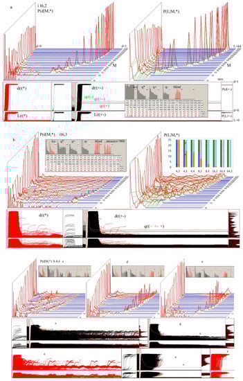
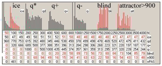
Figure 9.
Examples of the main results of growth simulations of open networks in aspect of half-chaos maintenance. These images are combinations of more important elements of screenshots, where the dynamic state of the simulation is shown in pixels. The qualitative nature of the results obtained at the end of the simulation is important here, but not the exact values of the results. This character is visible even in the incomplete image resolution; however, in the electronic version of this publication, the image can be enlarged to full resolution. For the clarity of the graphs of the table, the enlarged table of b has been added at the end with a supplementary description. Examples are taken from series with condition L; for series with condition d&L, no differences were found, but for series with condition d, many processes end in earlier stages M, while the rest is similar. Half-chaos is always present when the next acceptable change can be found in not too many attempts, therefore in series based on condition d for higher s and K, in many cases, modules destroy half-chaos. (a) Typical view of clearly half-chaotic evolution as an example of particular network i 16,2. For other parameters type, s, K, the view is very similar; only the place of ‘peninsula’ of Derrida’ chaotic equilibrium is shifted (see d or e for h 4,4). In a, there are more additional descriptions that are not repeated in (b–e). In upper row, P(d|M,*) and P(L|M,*) are shown. Here they are very similar. The beginning of growth, up to M of N = 400 to 500, is only a preparation of the network for later growth in stable conditions, therefore examination of half-chaos existence is performed on section N = 500 up to end in N = 4000. However, this initial section is important, because features of the network emerge that define its later behavior. For s,K = 4,2 up to N = 800, the effects of overlapping left and right peaks is typically visible. When s or K grow, this overlapping section ends earlier (in lower N). In the lower row, the ‘crocodiles’ are shown. Back crocodile d(t|+-) is drowned dynamically in one stage of growth, and here the last stage M (from N = 3500 to 4000) is shown. There are over 2000 attempts depicted of the addition and removal of nodes, therefore they blur some areas in black. For observation of details of the current process, the beginning section up to t = 100 for 20 cases are shown in the left; next, this window is cleaned. Between, in the grey area, all processes of functioning calculation from the beginning of network growth are left. On the left of the crocodile, the thresholds for d and L and upper limit of L crocodile are marked. On the right, after tmx, in the additional window, P(d) and P(L) are shown; however, only in the lower part of P. Vertical axis is d or L, like in crocodile. In black points, the addition case is depicted, while in red the removal case is shown. This is also repeated as the last M for N=4000 in the upper row. In black crocodile, q(t) is shown for addition, for removal, and for both of them. It is important that these q stabilize on a particular level that is clearly visible, which is the main feature of half-chaos. For normal chaos, q(t) monotonically drops down to zero. On the left of lower row, the beginning of red crocodile is given. It shows the effect of examination of obtained network after last stage M of growth (here for N = 4000) using point change of node function (depicted by *), as in method 4–7. It is similar to black crocodile, but some difference occurs (see c). To see these differences, red crocodiles were not cleaned before new black crocodiles are collected, therefore, especially in b, in black crocodiles, red elements of previous crocodile are visible. In (a), a stable area of black crocodile is used for important additional data: Level of ice, q for *,+,−, fraction of blind nodes, and number of attractors greater than 900, which were accepted, but their accumulation was blocked. Below there is a table of these data (*1000). These plots show them as a fraction of one (1 pixel = 1% if in black, or = 0.1% if in red). Such tables and plots from b are repeated on the end in enlarged form. Table shows results in detail, but it is added here to show our method only, while the qualitative form of plots over the table are important results and they are shown in each example. (b) Typical view of evolution blurred by growing modules as an example of particular network i 16,3. It is not the most blurred view, especially in P(d|M) distribution. Here mountain ridges built by growing modules are clearly visible. The right peak of Derrida’s chaotic equilibrium is low here, but still visible, similar in size to the ridges of the modules in which there is chaos. Modules emerge later but grow faster than Derrida equilibrium for the entire network. It is much more difficult to see it on P(L|M). Modules are visible in additional windows of crocodiles; however, in the main crocodile, the picture is blurred. In such a case, the ice clearly disappears; its appearance means there is a number of too long attractors, probably assembled from the few local attractors in simultaneously activated modules. Despite these modules over the threshold, q for all three types of initiating changes is high, therefore half-chaos exists. This q is also visible in black crocodile, typical for half-chaos stable form. In an empty place in P(L|M,*), a diagram of the share of categories ‘a’ (as in Figure a) and ‘b’ (as in Figure b) in the series L+ d&L, assembled by series with condition L (15 networks for each s,K) and condition d&L (10 networks), is included. Although categorizing a particular case to be similar to Figure a or to Figure b is problematic, statistics of such a result is important here, as it belongs to the main results of these qualitative investigations. (c–e). Different examples of h 4,4 networks evolutions. They are particular cases from one series, but what will we see when they are summarized? (c) Clear mountain ridges of growing modules emerge like in Figure b, and even ‘sea’ between is visible, but Derrida peninsula disappears. In black crocodiles, explosions in the chaos happen up to tmx; however, there is no Derrida equilibrium for the entire network, except in a module over the threshold. Despite this, q(t) is high and near stable. In the red crocodile, the view is different, but not very different. Here, explosion in the module chaos is less visible, but it is ‘thick’, because in this examination, there are no shifts of t in the initiation and many initiations use the same path. In black crocodiles, after each accommodation, initiation point t is also shifted to a similar path. In both crocodiles, second module is clearly visible on threshold level, while below it, clearance near the end emerges faster. This means this module melts by a higher explosion. Despite such effects, we can state that half-chaos is present here, but modules compete with it. In case c we include the category of ‘b’. (d) Derrida peninsula is clear; however, it is lower on the end where modules emerge. On the right of the crocodile, we can see at least two such modules. Classifying this case as ‘a’ or ‘b’ category is problematic, but this is a common problem for many cases. In black crocodiles, ‘v’ indicates the place, where a section of crocodile is cut off. (e) Another problematic case. Here a new module emerges in a non-typical place—on the end of Derrida peninsula. This module is clearly visible on the right of black crocodiles. Using only crocodiles, this case falls into category ‘a’, but in view of P(d|M), it is similar to Figure d, which is more problematic.
In the early stages of this investigation, an additional salvation mechanism through the return to some previous state was introduced. This mechanism changes obtained results from ‘evolutionary stability is always observed’ to a much weaker statement, ‘the path for evolutionary stability may be found’, which e.g., for living entities, means the same. However, this method turns out to be insufficient, and for larger s and K, most processes a reach dead end, which means no next evolutionary change (saving half-chaos) has been found and the only choice was to fall into chaos. However, the evolutionary process up to this point is not short, and there were a few alternative paths only checked in dangerous circumstances. There more probably earlier alternatives that may omit that problem, or some mechanisms may exist that help to avoid this problem. One such mechanism is to use the L condition instead of the d condition, but this changes the interpretation slightly. However, the first mechanism that limits half-chaos has been met. It is a separate mechanism, not an immanent feature of half-chaos. The process of evolution of real entities is assembled by many such independent mechanisms and each of them should be identified, separately investigated to be understood, and later estimated regarding its share in the visible effects of the observed process. Among them is half-chaos.
To find a reason for the problem with reaching the assumed Nmax, program B (a return below threshold is forbidden and the attractor must be less than 700 instead of 900) was applied, but it did not help much. Then we also checked this program for the series d&L+L, which was mentioned above. We expect that the problem lies in the structure of growing networks, where nearby outputs and inputs of the whole network (to environment) condense into hubs. Using condition L, the hubs near outputs cannot be changed, therefore they have less chance to be included in growing modules with chaotic behavior inside, even if the whole such module fits under the threshold d of the whole network. However, for proving such statements, a much wider analysis of collected data is necessary, as well as an additional investigation using the developed program.
4.3. Results and Discussion
The existence of half-chaos and its evolutionary stability in open networks is the problem investigated in ch.4 (met9). Earlier such existence was proven for autonomous networks with a constant structure (met4–7) [1,2,3,4,5] and for autonomous growing networks in ch.3 (met8) of this paper.
In previous methods (met4–8), the main result is P(d) where two clearly delimited peaks exist—‘left’ of the very small damage, containing a significant part of damage cases, and ‘right’ of the large damage, near the expected Derrida equilibrium of chaotic behavior. For an autonomous network, even if it is also growing and therefore does not possess stable N, results from consecutive stages of evolution (called ‘M’) may be summarized and shown in one chart. The presence of a constant number (here m = 64) of free inputs and outputs of the entire system results in an overlap of both watched peaks for small N (see [21,25,26]). Simultaneously with network growth, the modules grow even faster (see Figure 9b), which blurs the clear gap between peaks for larger N. Both these independent processes—network growth with half-chaos and module growth—are statistical, with large fluctuations for different networks. The sum of such effects gives a flat chart of P(d), which tells us almost nothing. Therefore, only the observation of a large number of particular P(d|M) for a particular network growth remains. Two main categories of such P(d|M) are shown in Figure 9a,b. There are 20 different evolution stages of M here. They are defined in a semi-logarithmic chain: N = 50, 100, 150, 200, 250, 300, 400, 600, 800, 1000, 1250, 1500, 1750, 2000, 2250, 2500, 3000, 3500, 4000. After each stage of evolution, by adding and removing nodes (noted as + or − in the figures), the state of the network is checked using not-accumulated initiation changes—the point change of node functions for one, as well as the current initial input state (noted as * in the figures). It is the same method as in met4–7.
Distributions P(d|M,+−*) and P(L|M,+−*) were collected as a screen dump (see Figure 9) and files of data for Excel, but summarizing such independent network evolutions gives inadequate results, which blurs important elements, e.g., the effects of growing modules. All types of initiations (+,−,*) lead to very similar views, then in Figure 9 for P(d|M) and P(L|M), only ‘*’ is used, but P(d|M) and P(L|M) differ slightly—more interesting details can be seen in P(d|M) (see Figure 9b).
Below P(d|M) and P(L|M), the crocodiles (red for * and back for +−) of d(t) and L(t) are shown. Moreover, in the form of a screen dump—the table and diagrams of ice, q of *+− the number of blind nodes and the number of global attractors that are greater than 900 and therefore were not accumulated are shown. More details can be found in the figure legend.
Such pictures of evolution of P(d) for consecutive M of one network are very different for diverse networks even with the same type, s,K, and condition (see Figure 9c–e). They are also different for L and d measures of damage, but similar for different types of initializing changes (* point change of function, + addition of node, − removal of node).
5. Conclusions
The main aim of this investigation was to answer the research question: Can half-chaos be present and how important is the role it plays in growing autonomous and open networks?
Half-chaos has been detected and demonstrated in autonomous networks of constant size and structure [1]. Checking its occurrence and role in the evolution of growing networks, in which the evolution of the structure is conditioned, is an important extension of the scope in which half-chaos should be considered as an important mechanism of evolution. This task is broken down into growing autonomous and open networks. In both cases examined separately due to technical conditions, half-chaos clearly occurs and persists for a long time, but it has a competitor in the form of growing modules, which, in the current model, destroys the half-chaos for larger s and K. (We use a number of equally probable signal variants s from 2 up to 64 and connectivity K (fixed number of inputs for each node in particular network) equal to 2, 3, or 4).
However, the current model does not include half-chaos control within modules, similar to the full network control. The extension of the model with such control should be the next step in the research of network evolution, but it requires solving several interpretation problems. The main one is to indicate which modules should be subject to such control and when.
Half-chaos is about how networks work inside a network, but the system is visible and judged through its outputs and inputs. The control of half-chaos through a small change in functioning is the basis of half-chaos, but it turns out that control through the amount of changes at the system outputs provides better results in keeping the half-chaos. Rather, this conclusion depends on the details of the model and should be further investigated. However, the method of checking through the system outputs is not a substitute for checking the functioning of the modules. We developed the simulation program in Pascal. We can send the full program by request.
The presented results represent an important source of subjects that await further research and solution.
Author Contributions
The topics met8 and met9, which are the content of the article, emerged naturally as the next stages of the A.G. research. The steps met1-met8 were performed by A.G., L.B.I. joined the discussion of met8 results, and met9 was undertaken jointly. The concept of met9 research was based on the experience of A.G., while L.B.I. did the main work on programming the simulations and carried out a significant part of it. The final results are presented, but they required many trial simulations, interpretation of their results, and corrections, which were discussed on an ongoing basis. All authors have read and agreed to the published version of the manuscript.
Funding
This research was supported by a grant of the Romanian National Authority for Scientific Research and Innovation, CCCDI-UEFISCDI, project number 101/2019, COFUND-CHISTERA-SOON, within PNCDI III. The article processing charge (APC) was funded by George Emil Palade University of Medicine, Pharmacy, Science and Technology of Targu Mures from Romania.
Institutional Review Board Statement
Not applicable.
Informed Consent Statement
Not applicable.
Acknowledgments
This work was developed in the framework of the CHIST-ERA programme supported by the Future and Emerging Technologies (FET) programme of the European Union through the ERA-NET Cofund funding scheme under the grant agreements, title: Social Network of Machines (SOON). This research was supported by a grant of the Romanian National Authority for Scientific Research and Innovation, CCCDI-UEFISCDI, project number 101/2019, COFUND-CHISTERA-SOON, within PNCDI III.
Conflicts of Interest
The authors declare no conflict of interest.
Appendix A
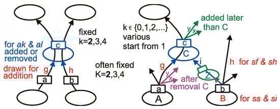
Figure A1.
Changeability patterns for ak and al (left), sh, sf, si, and ss network (right) depicted for K = 2. For addition of a new node to the network, links g and h are drawn. Node B is drawn instead of link h for ss and si. For K > 2 additional inputs are constructed like the ones on the right. For the removal of node, only a drawing of the node to remove is needed. The main moves are the same as for addition, but in an opposite sequence; however, for sh, sf, si, and ss, events that occur after the addition change the situation. Removal can create k = 0: Node Z added on link i can remain a k = 0 node while removing node C because part of link i from Z to remove C disappears. The outgoing links x,y, which were added to C after adding this node to the network, are moved to node A where link g starts. This lack of symmetry causes changes in distributions P(k) and other features of a network. For this reason, networks sf and ss with removals of node are different than without removal of node and are named sh and si, respectively [26] (Figure 2).
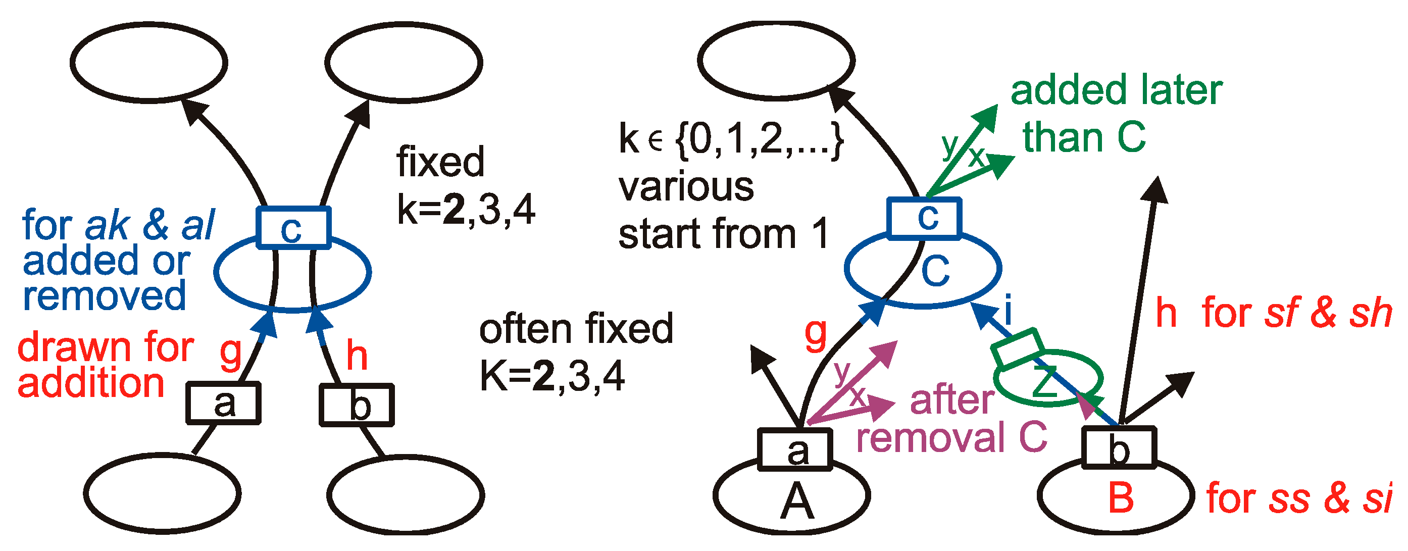
References
- Gecow, A. Life Is Not on the Edge of Chaos but in a Half-Chaos of Not Fully Random Systems. Definition and Simulations of the Half-Chaos in Complex Networks. In A Collection of Papers on Chaos Theory and Its Applications; Bracken, P., Uzumov, D.I., Eds.; IntechOpen: London, UK, 2021; p. 122. [Google Scholar] [CrossRef]
- Gecow, A. Life evolves in experimentally confirmed ‘half-chaos’ of not fully random networks, but not ‘on the edge of chaos’. In CHAOS 2020 Proceedings; Skiadas, C.H., Ed.; ISAST: Oakland, CA, USA, 2020; pp. 259–270. [Google Scholar]
- Gecow, A.; Nowostawski, M. Modelling Damage Propagation in Complex Networks: Life Exists in Half-Chaos. In Complex Networks XII. CompleNet-Live 2021; Teixeira, A.S., Pacheco, D., Oliveira, M., Barbosa, H., Gonçalves, B., Menezes, R., Eds.; Springer Proceedings in Complexity; Springer: Cham, Switzerland, 2021. [Google Scholar] [CrossRef]
- Gecow, A. Report of Simulation Investigations, a Base of Statement That Life Evolves in the Half-Chaos. 2016. Available online: http://vixra.org/abs/1603.0220 (accessed on 3 January 2022).
- Gecow, A. Report of Simulation Investigations, Part II, a Growth of Half-Chaotic Autonomous Networks. 2017. Available online: http://viXra.org/abs/1711.0467 (accessed on 3 January 2022).
- Derrida, B.; Pomeau, Y. Random Networks of Automata: A Simple Annealed Approximation. Europhys. Lett. 1986, 1, 45–49. [Google Scholar] [CrossRef]
- Derrida, B.; Weisbuch, G. Evolution of overlaps between configurations in random Boolean networks. J. Phys. 1986, 47, 1297–1303. [Google Scholar] [CrossRef] [Green Version]
- Kauffman, S.A. Requirements for Evolvability in Complex Systems—Orderly Dynamics and Frozen Components. Phys. D 1990, 42, 135–152. [Google Scholar] [CrossRef]
- Kauffman, S.A. The Origins of Order: Self-Organization and Selection in Evolution; Oxford University Press: New York, NY, USA, 1993. [Google Scholar]
- Kauffman, S.A. At Home in the Universe; Oxford University Press: New York, NY, USA, 1996. [Google Scholar]
- Albert, R.; Barabasi, A. Dynamics of Complex Systems: Scaling Laws for the Period of Boolean Networks. Phys. Rev. Lett. 2000, 84, 5660–5663. [Google Scholar] [CrossRef] [PubMed] [Green Version]
- Albert, R.; Barabási, A.-L. Statistical mechanics of complex networks. Rev. Mod. Phys. 2002, 74, 47–97. [Google Scholar] [CrossRef] [Green Version]
- Aldana, M.; Coppersmith, S.; Kadanoff, L.P. Boolean Dynamics with Random Couplings. In Perspectives and Problems in Nonlinear Science; Kaplan, E., Marsden, J.E., Sreenivasan, K.R., Eds.; Applied Mathematical Sciences Series; Springer: Berlin, Germany, 2003. [Google Scholar]
- Aldana, M. Dynamics of Boolean Networks with Scale Free Topology. Phys. D 2003, 185, 45–66. [Google Scholar] [CrossRef]
- Rämö, P.; Kesseli, J.; Yli-Harja, O. Perturbation avalanches and criticality in gene regulatory networks. J. Theor. Biol. 2006, 242, 164–170. [Google Scholar] [CrossRef]
- Fronczak, P.; Fronczak, A.; Hołyst, J.A. Kauffman Boolean model in undirected scale-free networks. Phys. Rev. E 2008, 77, 036119. [Google Scholar] [CrossRef] [Green Version]
- Nghe, P.; Hordijk, W.; Kauffman, S.A.; Walker, S.I.; Schmidt, F.J.; Kemble, H.; Yeates, J.A.M.; Lehman, N. Prebiotic network evolution: Six key parameters. Mol. BioSyst. 2015, 11, 3206–3217. [Google Scholar] [CrossRef]
- Gecow, A.; Hoffman, A. Self-improvement in a complex cybernetic system and its implications for biology. Acta Biotheor. 1983, 32, 61–71. [Google Scholar] [CrossRef] [PubMed]
- Gecow, A.; Nowostawski, M.; Purvis, M.K. Structural tendencies in complex systems development and their implication for software systems. J. UCS 2005, 11, 327–356. [Google Scholar]
- Gecow, A. Structural Tendencies - effects of adaptive evolution of complex (chaotic) systems. Int. J. Mod. Phys. C 2008, 19, 647–664. [Google Scholar] [CrossRef] [Green Version]
- Gecow, A. A certain complexity threshold during growth of functioning networks. In Proceedings of the 2008 First International Conference on Complexity and Intelligence of the Artificial and Natural Complex Systems. Medical Applications of the Complex Systems. Biomedical Computing, Tirgu Mures, Romania, 8–10 November 2008; pp. 69–76. [Google Scholar]
- Gecow, A. Emergence of Chaos and Complexity During System Growth. In From System Complexity to Emergent Properties; Aziz-Alaoui, M.A., Bertelle, C., Eds.; Understanding Complex Systems Series; Springer: Berlin, Germany, 2009; pp. 115–154. [Google Scholar]
- Gecow, A. Emergence of Growth and Structural Tendencies During Adaptive Evolution of System. In From System Complexity to Emergent Properties; Aziz-Alaoui, M.A., Bertelle, C., Eds.; Understanding Complex Systems Series; Springer: Berlin, Germany, 2009; pp. 211–241. [Google Scholar]
- Gecow, A. The conditions of structural tendencies. In Modelling and Analysis of Complex Interacting Systems; Aziz-Alaoui, M.A., Bertelle, C., Eds.; DCDIS-B Special Issue; Watam Press: Waterloo, ON, Canada, 2009; pp. 551–572. [Google Scholar]
- Gecow, A. Complexity Threshold for Functioning Directed Networks in Damage Size Distribution. 2010. Available online: https://arxiv.org/abs/1004.3795 (accessed on 3 January 2022).
- Gecow, A. Emergence of Matured Chaos During Network Growth, Place for Adaptive Evolution and More of Equally Probable Signal Variants as an Alternative to Bias p. In Chaotic Systems; Tlelo-Cuautle, E., Ed.; Intech: London, UK, 2011; pp. 280–310. ISBN 978-953-307-564-8. [Google Scholar] [CrossRef] [Green Version]
- Grassi, G. Chaos in the Real World: Recent Applications to Communications, Computing, Distributed Sensing, Robotic Motion, Bio-Impedance Modelling and Encryption Systems. Symmetry 2021, 13, 2151. [Google Scholar] [CrossRef]
- Martínez-Giménez, F.; Peris, A.; Rodenas, F. Chaos on Fuzzy Dynamical Systems. Mathematics 2021, 9, 2629. [Google Scholar] [CrossRef]
- Wang, Q.; Robnik, M. Multifractality in Quasienergy Space of Coherent States as a Signature of Quantum Chaos. Entropy 2021, 23, 1347. [Google Scholar] [CrossRef]
- Manera, M. Perspectives on Complexity, Chaos and Thermodynamics in Environmental Pathology. Int. J. Environ. Res. Public Health 2021, 18, 5766. [Google Scholar] [CrossRef]
- Kauffman, S.A. Boolean systems, adaptive automata, evolution. In Discovered Systems and Biological Organization; Bienenstock, E., Fogelman-Soulie, F., Weisbuch, G., Eds.; Series F: Computer and System Sciences 20; Springer: New York, NY, USA, 1986. [Google Scholar]
- Kauffman, S.A.; Peterson, C.; Samuelsson, B.; Troein, C. Genetic networks with canalyzing Boolean rules are always stable. Proc. Natl. Acad. Sci. USA 2004, 101, 17102–17107. [Google Scholar] [CrossRef] [PubMed] [Green Version]
- Shmulevich, I.; Kauffman, S.A.; Aldana, M. Eukaryotic cells are dynamically ordered or critical but not chaotic. Proc. Natl. Acad. Sci. USA 2005, 102, 13439–13444. [Google Scholar] [CrossRef] [PubMed] [Green Version]
- Villani, M.; La Rocca, L.; Kauffman, S.A.; Serra, R. Dynamical Criticality in Gene Regulatory Networks. Complex. Hindawi 2018, 2018, 1–14. [Google Scholar] [CrossRef]
- Turnbull, L.; Hütt, M.-T.; Ioannides, A.A.; Kininmonth, S.; Poeppl, R.; Tockner, K.; Bracken, L.J.; Keesstra, S.; Liu, L.; Masselink, R.; et al. Connectivity and complex systems: Learning from a multi-disciplinary perspective. Appl. Netw. Sci. 2018, 3, 1–49. [Google Scholar] [CrossRef] [Green Version]
- Erdős, P.; Rényi, A. On the evolution of random graphs. In Publication of the Mathematical Institute of the Hungarian Academy of Science; Publication of the Mathematical Institute of the Hungarian Academy of Sciences: Budapest, Hungary, 1960; pp. 17–61. [Google Scholar]
- Barabási, A.-L.; Albert, R.; Jeong, H. Mean-field theory for scale-free random networks. Phys. A 1999, 272, 173–187. [Google Scholar] [CrossRef] [Green Version]
- Iantovics, L.B.; Enăchescu, C.; Filip, F.G. (Eds.) . Complexity in Artificial and Natural Systems; “Petru Maior” University Publishing House: Targu Mures, Romania, 2008; ISBN 978-973-7794-76-5. [Google Scholar]
- Iantovics, L.B.; Radoiu, D.; Marusteri, M.; Dehmer, M. (Eds.) Special Issue on Complexity. In Sciences and Artificial Intelligence; BRAIN. Broad Research in Artificial Intelligence and Neuroscience; EduSoft: Bacau, Romania, 2010; ISSN 2067-3957. [Google Scholar]
- Iantovics, L.B.; Hluchý, L.; Kountchev, R. (Eds.) Special Issue on Understanding Complex Systems; Acta Universitatis Apulensis: Alba Iulia, Romania, 2011; ISSN 1582-5329. [Google Scholar]
- Teixeira, A.S.; Pacheco, D.; Oliveira, M.; Barbosa, H.; Gonçalves, B.; Menezes, R. (Eds.) Complex Networks XII. CompleNet-Live 2021; Springer Proceedings in Complexity; Springer: Cham, Switzerland, 2011. [Google Scholar]
- Skiadas, C.H.; Dimotikalis, Y. (Eds.) 13th Chaotic Modeling and Simulation International Conference; Springer Proceedings in Complexity; Springer: Cham, Switzerland, 2021; ISSN 2213-8684. [Google Scholar]
- Altenberg, L. Modularity in Evolution: Some Low-Level Questions. In Modularity: Understanding the Development and Evolution of Natural Complex Systems; Callebaut, W., Rasskin-Gutman, D., Eds.; The Vienna Series in Theoretical Biology; MIT Press: Cambridge, MA, USA, 2005; pp. 99–128. [Google Scholar]
- Sun, H.; Jie, W.; Loo, J.; Wang, L.Z.; Ma, S.G.; Han, G.; Wang, Z.M.; Xing, W. A parallel self-organizing overlapping community detection algorithm based on swarm intelligence for large scale complex networks. Futur. Gener. Comput. Syst. 2018, 89, 265–285. [Google Scholar] [CrossRef]
- Kauffman, S.A. Metabolic stability and epigenesis in randomly constructed genetic nets. J. Theor. Biol. 1969, 22, 437–467. [Google Scholar] [CrossRef]
- Luque, B.; Sole, R.V. Phase transitions in random networks: Simple analytic determination of critical points. Phys. Rev. E 1997, 55, 257–260. [Google Scholar] [CrossRef] [Green Version]
- Serra, R.; Villani, M.; Graudenzi, A.; Kauffman, S.A. Why a simple model of genetic regulatory networks describes the distribution of avalanches in gene expression data. J Theor. Biol. 2007, 246, 449–460. [Google Scholar] [CrossRef] [PubMed]
- Sole, R.V.; Luque, B.; Kauffman, S. Phase Transitions in Random Networks with Multiple States; Technical Report 00-02-011; Santa Fe Institute: Santa Fe, NM, USA, 2000. [Google Scholar]
- Serra, R.; Villani, M.; Semeria, A. Genetic network models and statistical properties of gene expression data in knock-out experiments. J. Theor. Biol. 2004, 227, 149–157. [Google Scholar] [CrossRef] [PubMed]
- Ishii, M.; Gores, J.; Teuscher, C. On the sparse percolation of damage in finite non-synchronous random Boolean networks. Phys. D (Nonlinear Phenom.) 2019, 393, 84–91. [Google Scholar] [CrossRef]
- Escobar, L.A.; Kim, H.; Gershenson, C. Effects of Antimodularity and Multiscale Influence in Random Boolean Networks. Complexity 2019, 2019, 1–14. [Google Scholar] [CrossRef] [Green Version]
- Pontes-Filho, S.; Lind, P.; Yazidi, A.; Zhang, J.H.; Hammer, H.; Mello, G.B.M.; Sandvig, I.; Tufte, G.; Nichele, S. A neuro-inspired general framework for the evolution of stochastic dynamical systems: Cellular automata, random Boolean networks and echo state networks towards criticality. Cogn. Neurodyn. 2020, 14, 657–674. [Google Scholar] [CrossRef]
- Serra, R.; Villani, M.; Agostini, L. On the dynamics of random Boolean networks with scale-free outgoing connections. Phys. A 2004, 339, 665–673. [Google Scholar] [CrossRef]
- Iguchi, K.; Kinoshita, S.-I.; Yamada, H.S. Boolean dynamics of Kauffman models with a scale-free network. J. Theor. Biol. 2007, 247, 138–151. [Google Scholar] [CrossRef] [PubMed] [Green Version]
- Tez, M. Genome’s Chaotic Behavior for Adaptation may explain Carcinogenesis! Suggestion from Surgical Oncologist. J. Cancer Biol. Res. 2014, 2, 1047. [Google Scholar]
- Tez, M. Organismic Perspective of Carcinogenesis. 2021; preprint. [Google Scholar] [CrossRef]
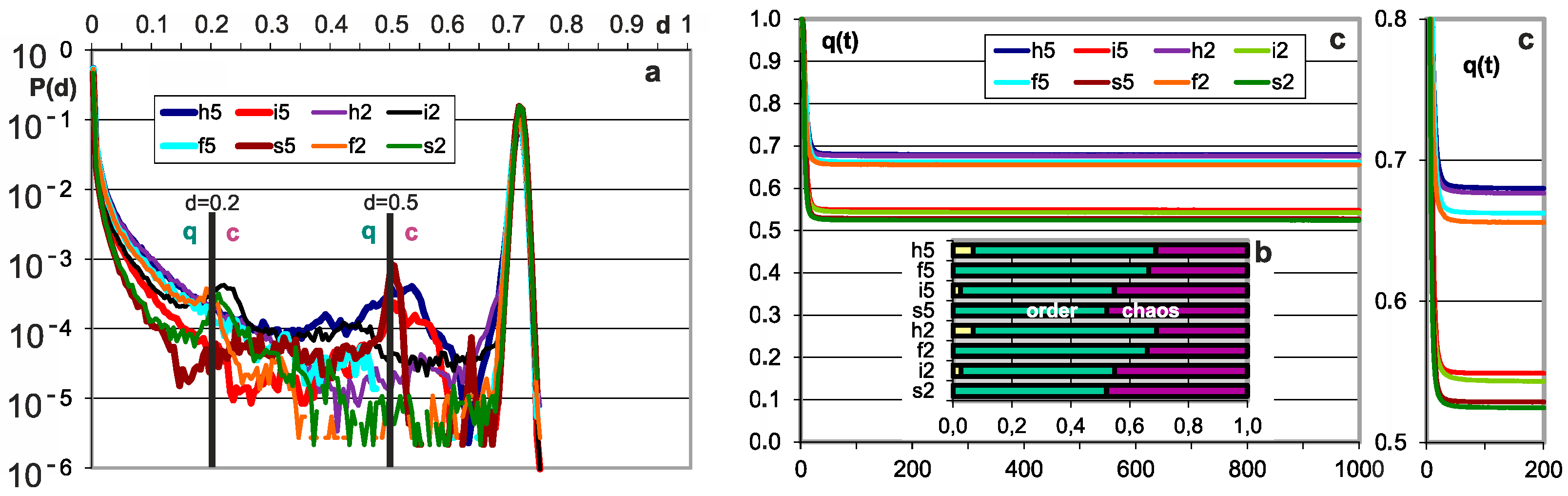
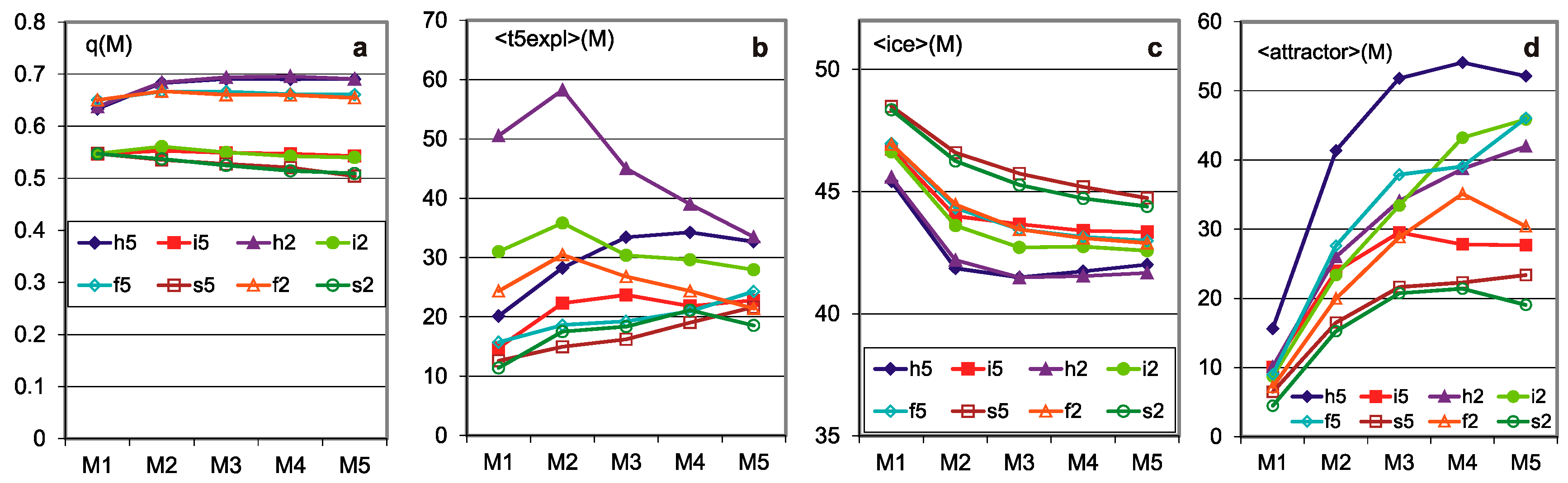
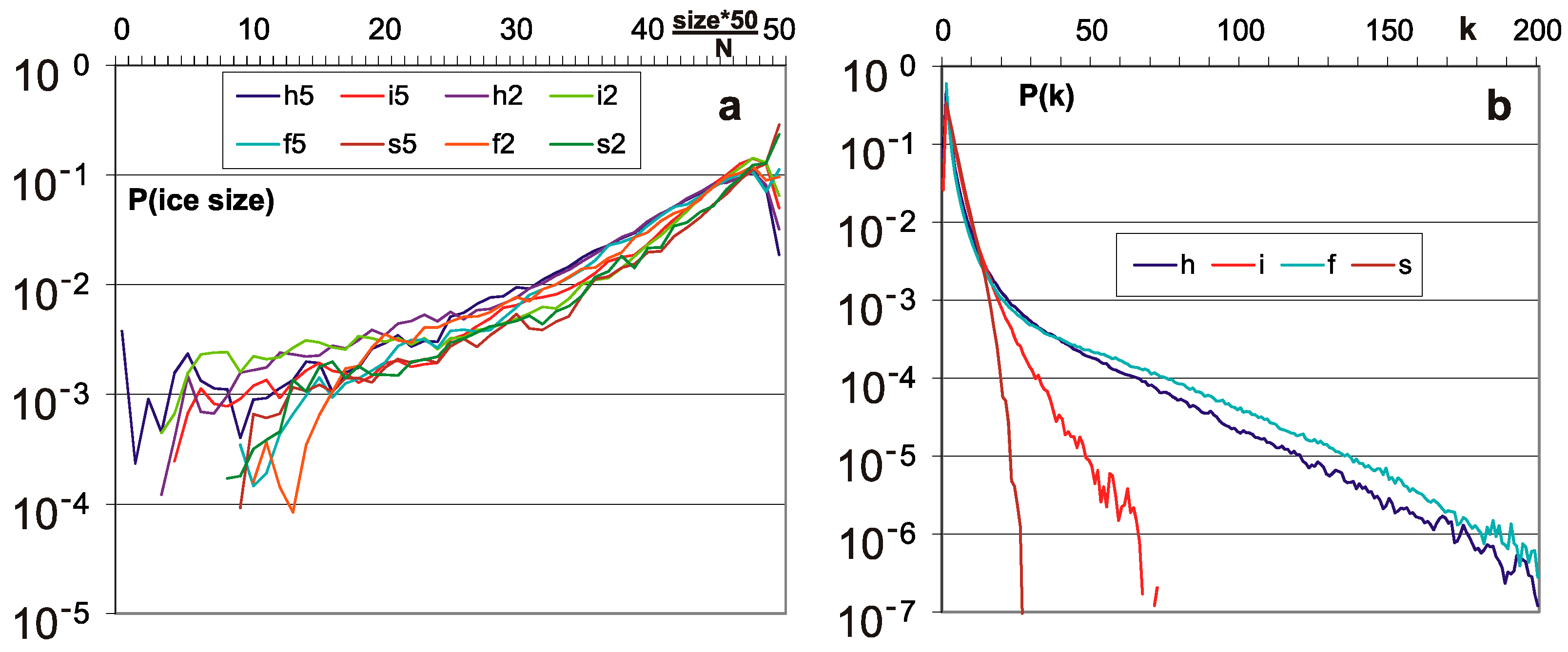

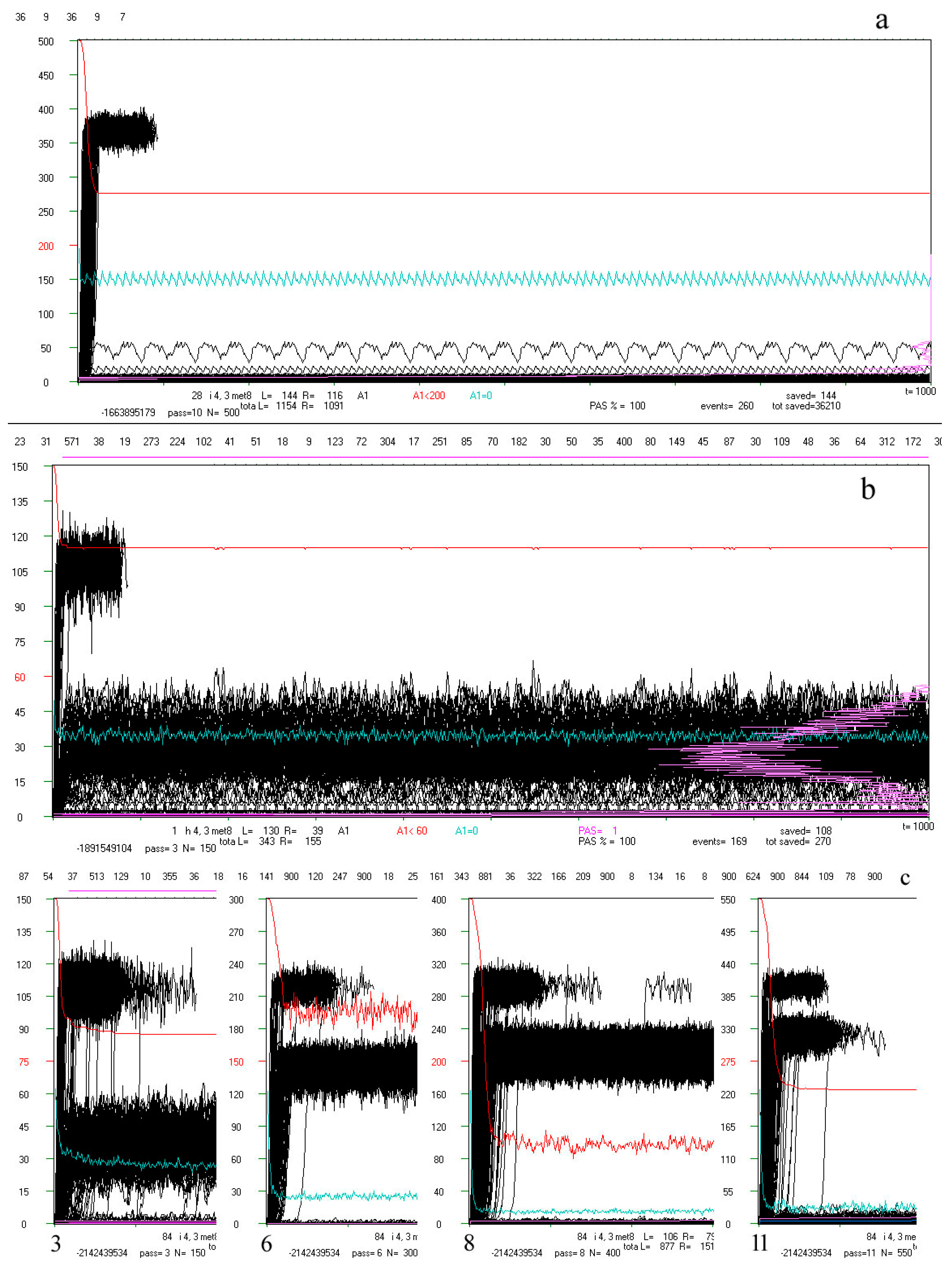
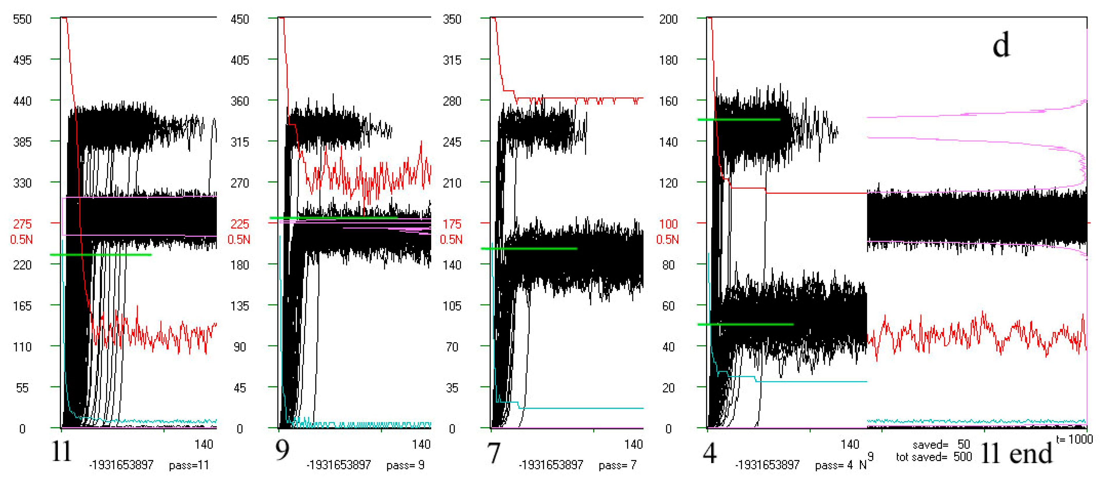
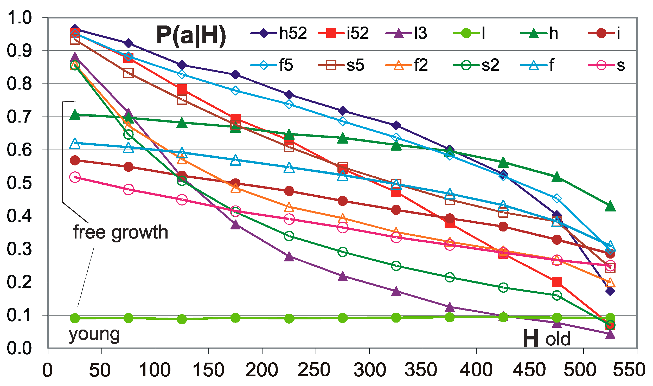
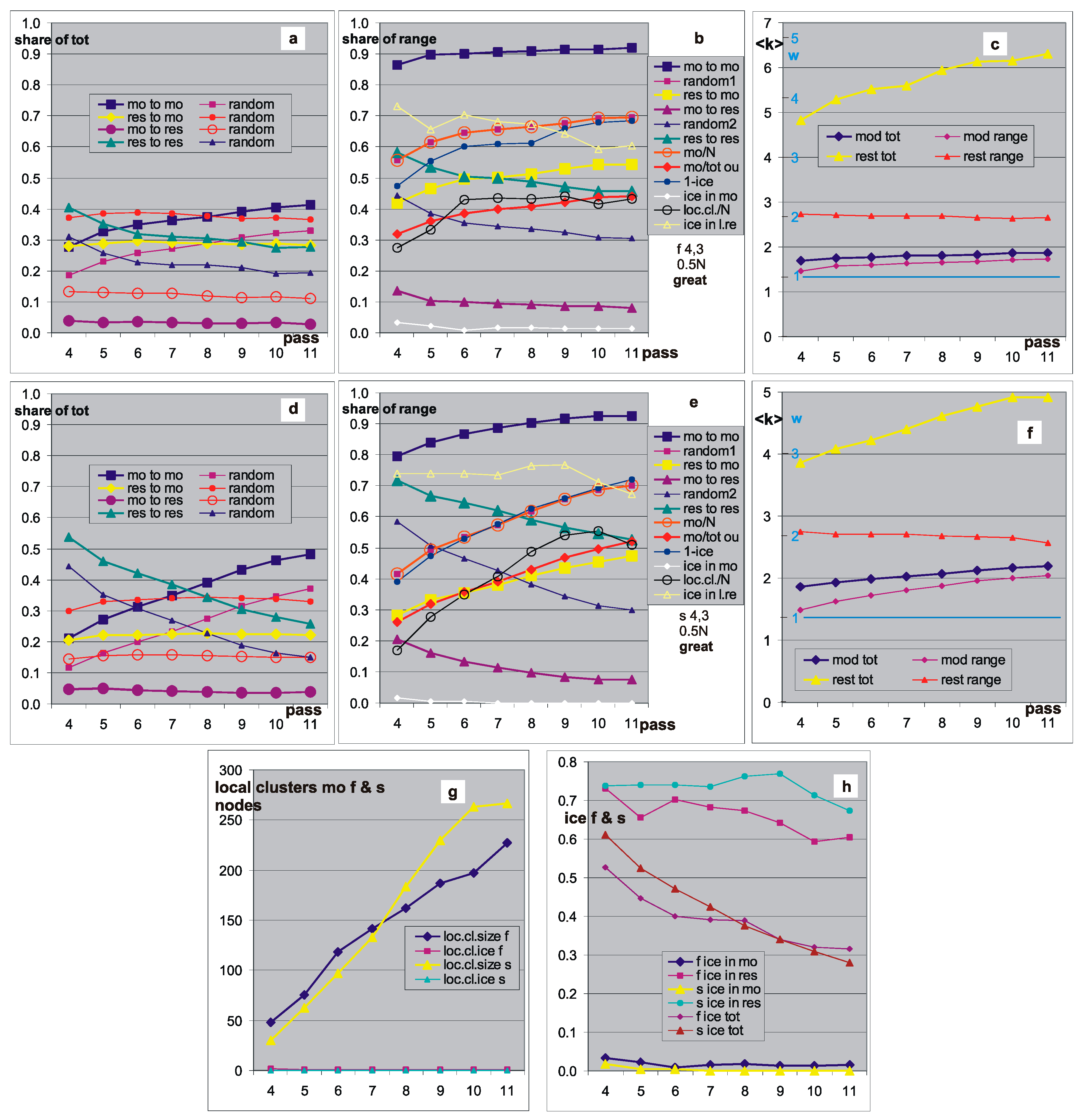
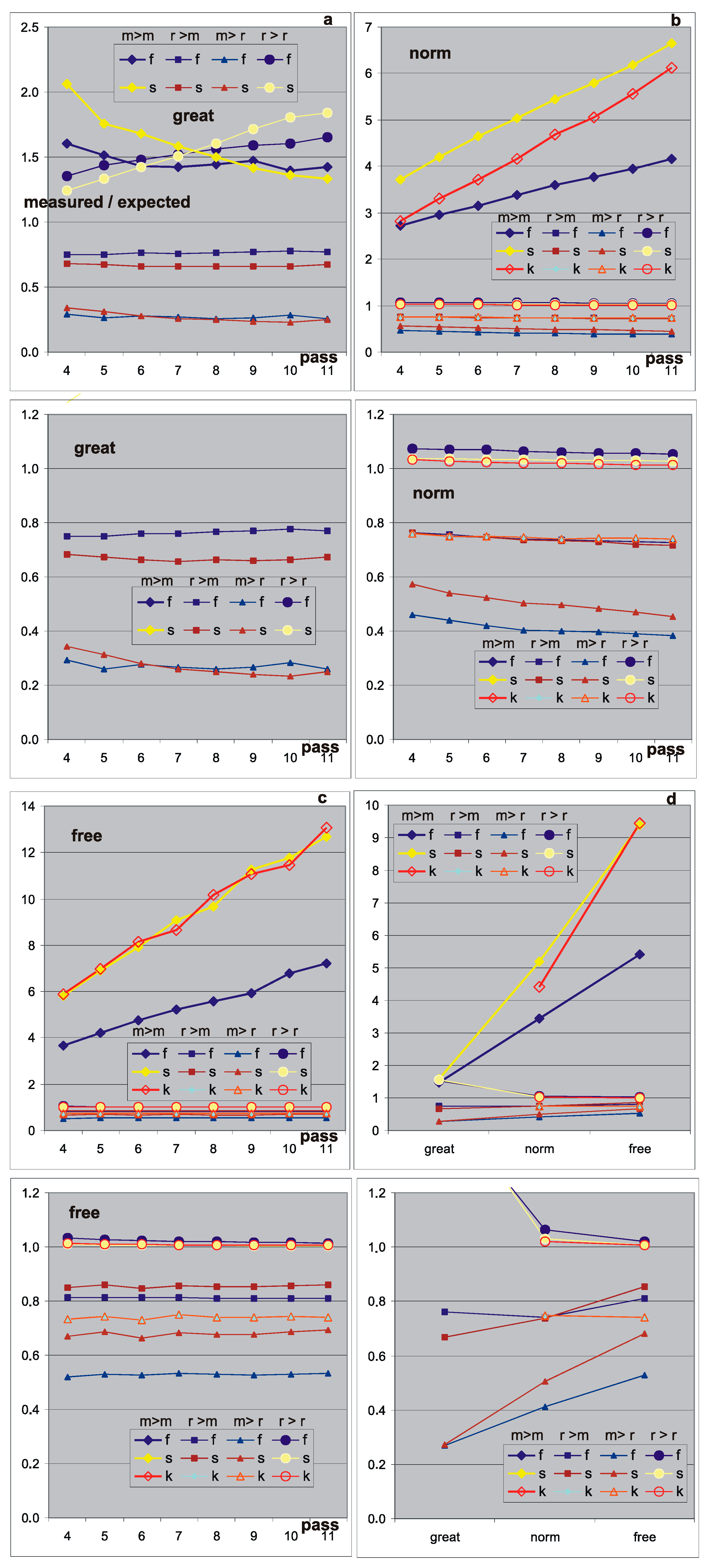
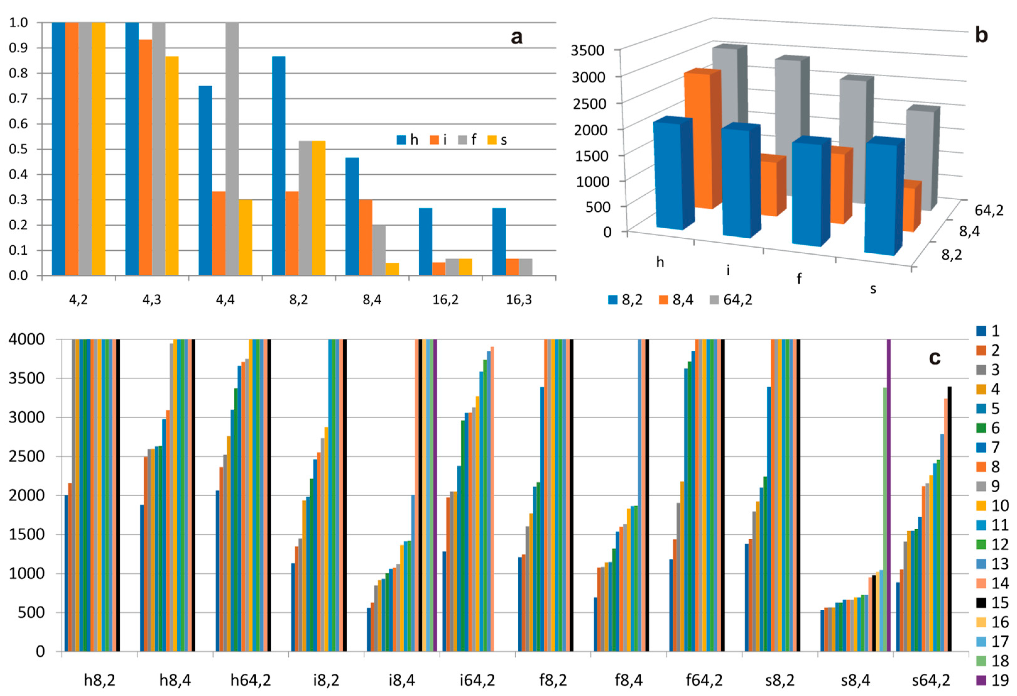

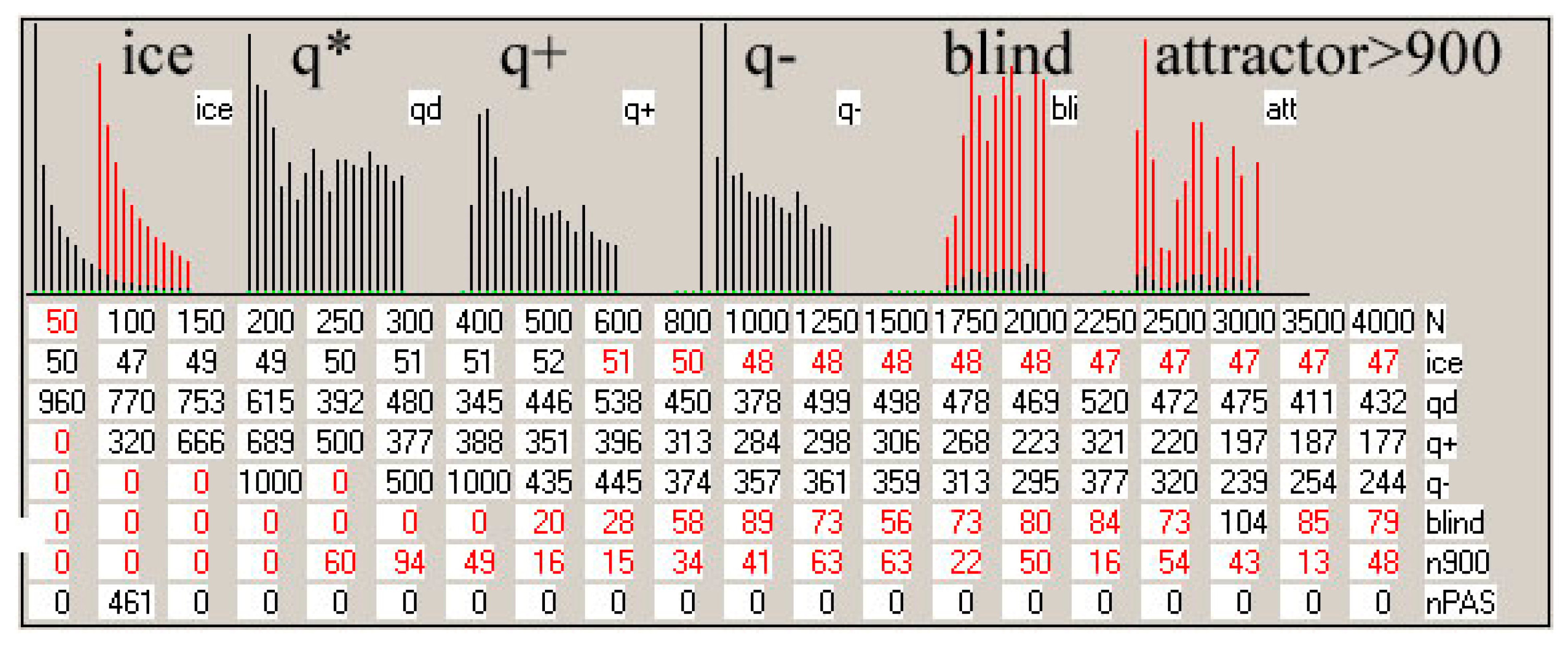
Publisher’s Note: MDPI stays neutral with regard to jurisdictional claims in published maps and institutional affiliations. |
© 2022 by the authors. Licensee MDPI, Basel, Switzerland. This article is an open access article distributed under the terms and conditions of the Creative Commons Attribution (CC BY) license (https://creativecommons.org/licenses/by/4.0/).