Abstract
The vibration signal of the shearer is one of the important signals for coal and rock cutting mode recognition and fault diagnosis. However, the signal collected in the field contains a large amount of background noise, which is not conducive to subsequent analysis and processing. Therefore, a noise elimination method for coalcutter vibration signal based on Ensemble Empirical Mode Decomposition (EEMD) and an Improved Harris Hawks Optimization (HHO) algorithm is proposed in this paper. The vibration signal is first decomposed by EEMD to generate a series of intrinsic mode functions (IMF). The HHO algorithm was introduced to determine the optimal denoising threshold of each IMF. In addition, the original HHO has been improved to use the natural constant as the base exponential function to determine the escape energy trend line. Simulation results show that compared with the other four denoising methods, the signal waveform processed by this method is smoother. Under different types of signals and the same intensity of noise, the SNR increases by 70.9%, 6.7%, 2.6%, and 10.53% on average, respectively. The MSE decreases by 67.6%, 12.7%, 4.5%, and 5.42% on average. Under the same type of signal and different intensity of noise environment, the SNR is improved by 74.62%, 37.70%, 5.24%, and 39.72% on average, respectively. MSE decreased by 77.38%, 53.10%, 9.88%, and 54.67% on average. Finally, the method is applied to the shearer working state diagnosis system, and its actual effect is verified.
1. Introduction
The coal shearer is one of the key pieces of equipment in realizing the safe and efficient production of coal mines and is the main component of fully mechanized mining equipment. Its intelligence level is the key factor in realizing the “unmanned” or “less humanized” aspect of the fully mechanized mining face [1,2]. In the actual operation process, because the cutting roller and the coal wall contact directly, the shearer cutting the coal wall will cause complex vibration of the whole machine. Different geological conditions of coal seams will inevitably lead to different vibration characteristics of the rocker’s arm. A large number of field investigations and theoretical studies show that the common fault of shearer, engine, gas turbine, and other rotating machinery results from vibration. This vibration seriously restricts the development of industry [3,4]. Therefore, many scholars in this field have conducted a large number of analyses and numerical and experimental studies on its vibration characteristics to improve the accuracy of pattern recognition and fault detection [5,6]. In addition, the vibration signal measurement system has a lower cost and simpler structure. However, the vibration signals of the rocker’s arm collected in the field are all mixed vibration signals. There are a lot of noise components in the initial vibration signals. Therefore, the denoising operation is indispensable, and the quality of denoising performance directly affects the effect of subsequent processing.
The working environment in the mine is special, and the collected vibration signal of the rocker’s arm is a nonlinear and non-stationary signal [7]. It is very important to find a suitable denoising method. The basis function and decomposition level of EMD are generated according to the processed signal, and the adaptability to the signal is very strong [8]. Therefore, this method has advantages for dealing with non-stationary and nonlinear complex signals [9]. On the basis of EMD, Z. Wu et al. proposed Ensemble Empirical Mode Decomposition (EEMD) [10]. In this method, tens to hundreds of EMD processes are performed on a signal, and different white noise is added to each EMD. The mode mixing phenomenon existing in EMD is effectively suppressed, and the accuracy of signal processing is improved [11]. Jeffery C. Chan et al. proposed a denoising method based on EEMD and automatic thresholding [12]. This method generates automatic thresholds based on mathematical morphology to achieve noise elimination. In [13], a denoising method based on EEMD and an improved general threshold were proposed. This method modifies the threshold value according to Spearman’s rho and achieves good results.
Although the above methods have achieved good results, most of these methods use mathematical estimation, experience, and experiments. For complex and changeable signals, it is difficult to obtain the best denoising effect [14]. In recent years, benefiting from the development of intelligent optimization algorithms, the approach of using intelligent optimization algorithms to search for thresholds has been gradually adopted. An adaptive ECG signal denoising method based on EEMD and genetic algorithm was proposed by Phuong Nguyen et al. [15]. The performance of this method was evaluated in the MIT-BIH arrhythmia ECG database, and the effect was demonstrated. In [16], Shweta Jain et al. compared the denoising effect of thresholds selected by various optimization algorithms on electrocardiogram signals. The results show that cuckoo search optimization algorithms can achieve maximum signal-to-noise ratio (SNR) and minimum mean square error (MSE). In [17], Qian Zhang et al. used the particle swarm optimization algorithm to search for the denoising threshold of the IMF with noise. The aim is to improve the SNR by more than 14 dB in the field of sensing fiber optic signal transmission.
Harris Hawks Optimization (HHO) algorithm was a new bio-intelligent optimization algorithm proposed by Ali Asghar Hei-Dari et al. in 2019 [18]. The main inspiration for HHO comes from the cooperative hunting behavior of the Harris’s hawk population in nature. The desert predator demonstrates the naturally evolved strategic ability to track, surround, and eventually raid [19]. Compared with other existing metaheuristic algorithms, HHO has higher search accuracy, simpler structure, and fewer parameters. It is widely used in pattern recognition, neural network parameter optimization, signal extraction, and other fields [20]. However, the HHO algorithm also has some limitations. For example, it is easy to fall into a local optimal solution, and a “premature phenomenon” occurs [21]. Many improvement methods have been proposed. In [22], Vikram Kumar Kamboj et al. introduced hybrid variants and sine–cosine development algorithms and created a hybrid Harris Hawks sine–cosine algorithm. The optimization algorithm is effective for various nonlinear, non-convex, and highly constrained engineering design problems. The periodic variation mechanism was adopted to improve the original HHO [23]. It was applied to the field of fault diagnosis and had a better diagnostic performance. In [24], Hussain K. et al. introduced a new modified variant with the concept of long-term memory and proposed the long-term memory Harris Hawks Optimization algorithm. It has good optimization accuracy. In recent years, many improvements have been made to HHO, but few researchers have been able to balance the exploration stage and exploitation stage.
A noise elimination method for coalcutter vibration signal based on Ensemble Empirical Mode Decomposition and an improved Harris Hawks Optimization algorithm is proposed in this paper. To determine the optimal denoising threshold of each IMF after EEMD decomposition, HHO is introduced into the threshold selection process of this denoising method. In addition, the escape energy trend line determined by the linear function in the original HHO was replaced by that determined by the exponential function. The global exploration and local development processes of the original HHO are balanced to avoid falling into the local optimum and improve the convergence accuracy of the algorithm. The rest of this paper is organized as follows. In Section 2, the basic EEMD noise removal method and the basic theory of HHO are introduced. In Section 3, The improved HHO (IHHO) for the escape energy trend line determined by the exponential function, and the denoising process based on EEMD and IHHO (EEMD-IHHO) are presented in detail. In Section 4, the effectiveness and superiority of the method are verified under different types of signal and different intensity noise environments. In Section 5, The proposed EEMD-IHHO is used to denoise the coal-rock cutting vibration signal of the coal shearer, and the practical application effect is verified. Some conclusions and outlooks are summarized in Section 6.
2. Basic Theory
2.1. Denoising Based on EEMD
EEMD is a method for analyzing nonlinear and nonstationary data. The most important feature is that the mode mixing phenomenon in EMD is suppressed by adding white Gaussian noise to the signal. Therefore, the accurateness and completeness of signal processing is further improved. As with EMD, each IMF generated by EEMD needs to meet two basic conditions. The difference between the number of zeros and extreme points is either zero or one in each function. Furthermore, the upper and lower envelopes are fitted by local maxima and local minima, and their mean line is zero at any point. The key process of EEMD is described below.
The NE times of white Gaussian noise are added to the signal in EEMD. The ratio of the standard deviation of the added white noise to the standard deviation of the original signal is denoted as Nstd. Then, NE times EMD decomposition is performed. The average of IMFs and residuals of the same order at different times is calculated. Finally, the average IMFs and residual are obtained. The decomposition result can be expressed by Equation (1).
where is the residual component. It represents the average change trend of .
Inspired by the wavelet threshold denoising method, many scholars have tried a series of denoising methods based on EEMD. At present, the general method of calculating fixed threshold proposed by Donoho and Johnstone is mostly adopted [25]. Before calculating the threshold, it is necessary to obtain the noise variance. Therefore, Equation (2) is used to calculate:
where, is the noise standard deviation of the j-th IMF after EEMD decomposition of signal data . is the absolute median deviation of the j-th IMF. is the length of the signal.
The fixed threshold method is used to calculate the threshold of each IMF, as shown in Equation (3):
A soft threshold or hard threshold denoising function is used for denoising. Equations (4) and (5) are as follows:
where is the threshold corresponding to the j-th IMF. is the coefficient of the j-th IMF at time t. is the coefficient of the j-th IMF at time t after being processed. Sgn is a symbolic function.
It can be seen from the hard threshold function that some coefficients remain at the original value while the other coefficients become zero directly. Therefore, denoising signals are discontinuous and have oscillatory phenomena [26]. However, the absolute value of one part of the coefficient of the soft threshold function decreases, and the other part of the coefficient is zero. This processing maintains the continuity of denoised signals, and most researchers use soft threshold functions for denoising [27].
The reconstructed signal includes the denoised IMF and residual, which can be expressed by Equation (6):
where is the signal denoised by EEMD. is the denoised order IMF.
2.2. Harris Hawks Optimization Algorithm
HHO algorithm was a natural heuristic algorithm proposed by Heidari et al. in 2019 [18]. It was inspired by the collaborative foraging behavior of the Harris’s hawk. Harris’s hawks are found in southern Arizona. They efficiently perform cooperative foraging in several stages including pursuit, siege, and attack. This optimization algorithm is developed by mathematically simulating the dynamic pattern and behavior [28]. This algorithm has the advantages of a single parameter, easy implementation, and good robustness. Therefore, it is widely used in pattern recognition, neural network parameter optimization, signal extraction, and other fields. Its operation process includes three stages, namely the exploration stage, transition stage, and exploitation stage.
- (1)
- Exploration Stage
In the exploration stage, the Harris’s hawks stop at random locations and wait to find prey according to two strategies. The two strategies are as equations corresponding to and .
where represents the position vector in the t-th iteration. refers to the position of the prey. refers to the current position vector. , , , and are all randomly generated in , and are the upper and lower bounds of all positions respectively. refers to a random location. is the average position, which can be obtained by Equation (8).
where refers to the current position of the i-th Harris’s hawk, and is the total number of groups.
- (2)
- Transition Stage
In HHO, a monotonically decreasing linear function is used to simulate the overall trend line of prey escape energy over time, as in Equation (9).
where represents the maximum number of iterations. Therefore, the escape energy of the prey is denoted by Equation (10):
where E0 is called the initial energy of the prey. is updated in (−2, 2) at each iteration.
When , the HHO algorithm executes the exploration stage. When , the HHO algorithm performs the exploitation stage.
- (3)
- Exploitation Stage
At this stage, the HHO algorithm simulates four hunting methods, namely soft siege, soft siege with progressive dive, hard siege with progressive dive, and hard siege.
- Soft siege with progressive dive: when and , the energy of the prey is sufficient. The chance of escape is also high. There are two ways to update the position of each Harris’s hawk. One way is simulated by Equation (11).
To imitate this real hunting phenomenon, the levy flight function is introduced, as shown in Equation (12).
where , are random values between (0, 1). Another way is expressed by Equation (13).
where is the search space dimension, and is a D-dimensional random vector.
Therefore, the soft siege with progressive dive can be simulated by Equation (14):
- b.
- Soft siege: when and , the prey still has sufficient physical strength. At this time, the Harris’s hawks slowly surround the prey to consume their energy. The formula is as follows.
- c.
- Hard siege with progressive dive: when and , the prey does not have enough energy to escape. This strategy has two ways of updating the position, as follows:
- d.
- Hard siege: when and , the prey is already very tired. Harris’s hawks quickly formed in a small encircle. The position change of Harris’s hawk is shown in Figure 1 [29], which is simulated by Equation (20).
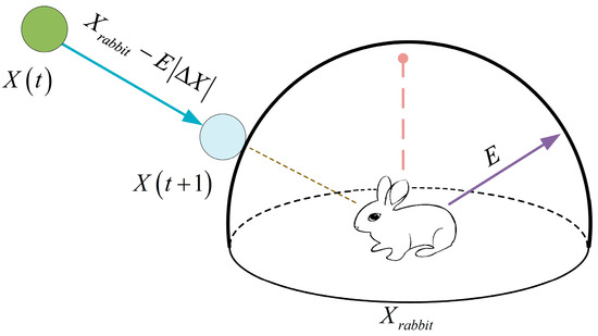 Figure 1. A Harris’s hawk’s position changes.
3. Proposed Method
3.1. Improvement of HHO
According to the original HHO, the changing trend of escape energy is determined by a simple linear decay function. When the number of iterations is 500, the change of escape energy of running HHO twice is shown in Figure 2. As can be seen from Figure 2, the exploration stage of the first half of the algorithm is strong enough for global search. However, the second half of the iterative process only performs the exploitation phase, not the exploration phase. When the optimal solution is too far away from the convergent group, it is easy to fall into the local optimal solution. Therefore, the escape energy is modified.
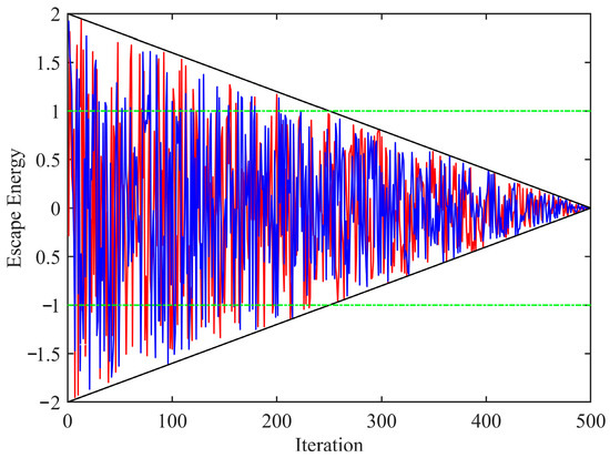
Figure 2.
Change of in HHO before improvement.
The improvement is mainly based on two points. The first point is to balance the exploration phase and exploitation phase. In the exploration phase, the escape energy should be reduced slowly to maintain the advantage of the algorithm with large global search ability. In the later development stage of iteration, the algorithm is given the possibility of a global search to avoid falling into the local optimum. The second point is to ensure the convergence of the HHO algorithm. The escape energy is theoretically equal to 0 at the last iteration. This makes the local exploration more thorough in order to improve the optimization accuracy. Therefore, the original escape energy trend line is replaced by the escape energy trend line determined by the exponential function , as shown in Equation (21):
where is determined by experiment. is the maximum number of iterations. Equation (22) is the calculation formula of escape energy.
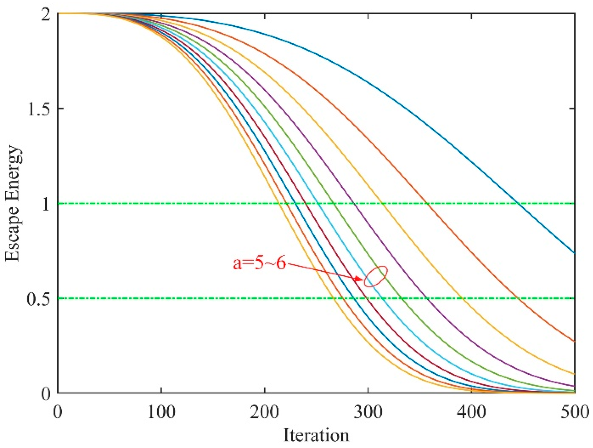
When T = 500, the parameter in Equation (21) was tested with different values. As shown in Figure 3, the escape energy trend lines from top to bottom correspond to respectively. When , the trend line of escape energy is not close to 0 at the end of the iteration. It can be seen from the exploitation stage of Harris’s hawks, which leads to incomplete development and reduced optimization accuracy. When , it can be seen from the trend line of escape energy that the algorithm retains the advantage of a large global search in the early stage. However, in the later stage of the algorithm, the possibility of the global search is still weak when it gradually transitions to the exploitation stage. In addition, in the exploitation stage, escape energy is an important basis for the selection of four hunting strategies. If or , the iterations accounted for by a large difference will lead to the unbalanced selection of the four hunting strategies. It will cause the search location points in a certain area to be too dense or evacuated, and to ignore the optimal location points. To sum up, the value of ranges from 5 to 6.
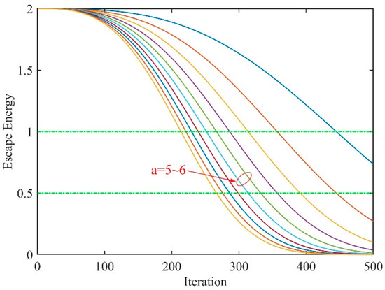
Figure 3.
Escape energy trend line with from 1 to 10.
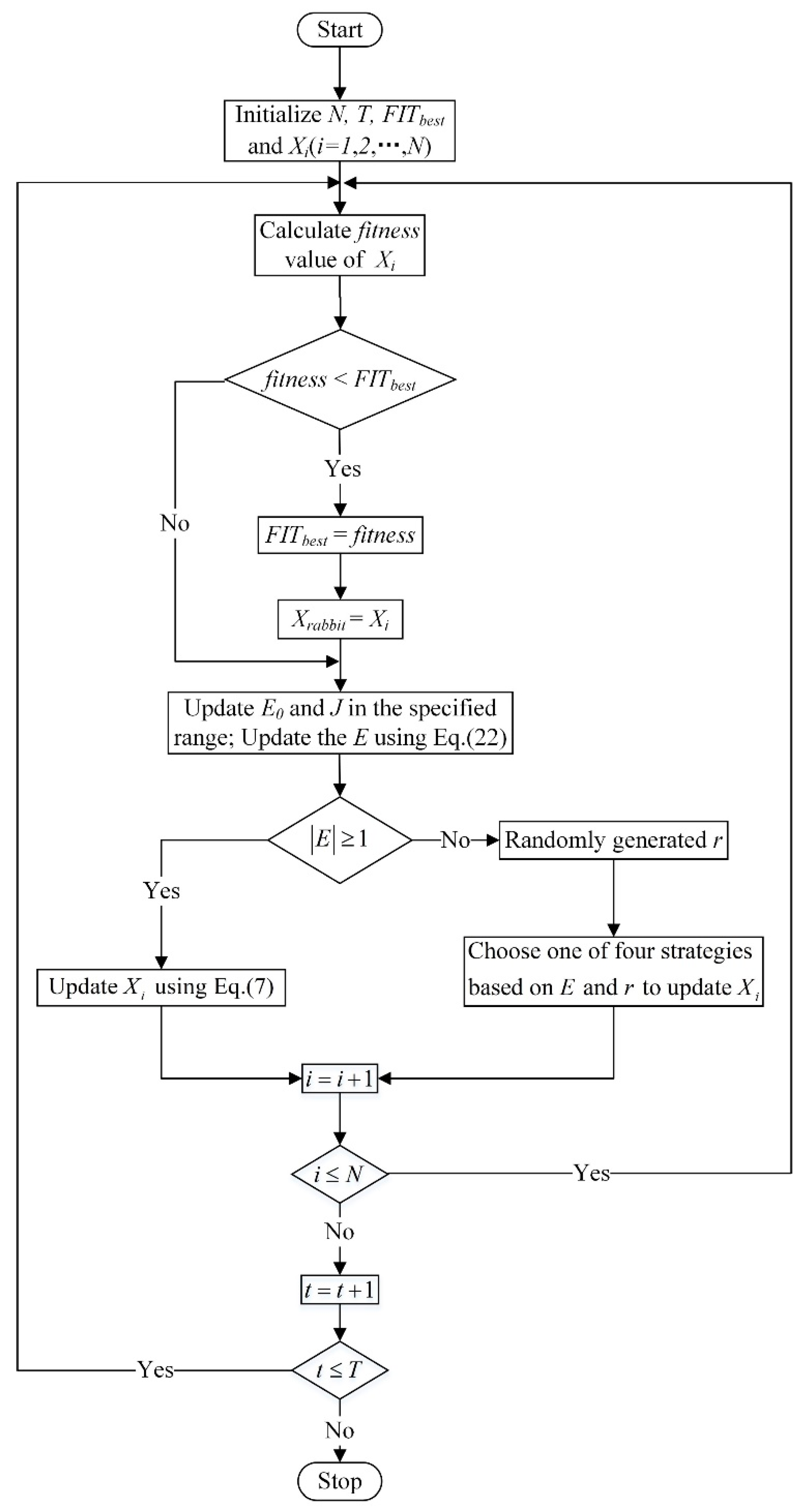
Figure 4 shows the escape energy diagram after two improved runs at = 5 and = 600. As can be seen from Figure 4, the improved escape energy preserves the advantage of large exploration ability in the early stage of the algorithm. It also endows the possibility of global search in the later stage of the algorithm to avoid falling into local optimum. On the other hand, the four kinds of trapping strategies in the exploitation stage are balanced to fully search every location area and improve the convergence accuracy. The procedure block diagram of the IHHO is shown in Figure 5. Where represents the initial fitness value.
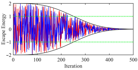
Figure 4.
Change of in HHO after improvement.
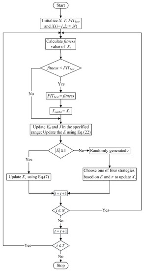
Figure 5.
Procedure block diagram of the IHHO.
3.2. Flow of the Proposed Denoising Method
According to the theoretical basis mentioned above, this paper proposes a noise elimination method for coalcutter vibration signal based on Ensemble Empirical Mode Decomposition and an improved Harris Hawks Optimization algorithm. This method is abbreviated as EEMD-IHHO. In this method, the signal-containing noise is first decomposed into several IMFs by EEMD. Then, the IHHO algorithm is used to find the optimal threshold. Finally, each IMF coefficient is contracted by the soft threshold function. The IMFs are reconstructed to obtain the final signal. The specific process of this method is described below:
Step 1: Parameter initialization. Such as , , , , . Positions of each Harris’s hawk. Each represents a threshold feasible solution in this algorithm.
Step 2: Signal decomposition. EEMD decomposes the original noisy signal into several IMFs and a residual, which can be expressed as .
For the actual denoised signal, a pure useful signal cannot be extracted. Therefore, the denoised signal-to-noise ratio cannot be calculated and the denoising effect cannot be evaluated. Thus, based on the signal independence theory, the original noise signal can be expressed as a useful signal and a noise signal , namely . The fitness function is established, as in Formula (23) [30].
where is the second-order correlations coefficient and is the higher-order correlations coefficient. If and decrease at the same time, it means that the useful signal is gradually separated from the noise signal [31].
where is the covariance coefficient, .
Step 3: Threshold optimization. Firstly, the fixed threshold obtained by Equation (6) is slightly enlarged as the upper bound of the IHHO search range. The lower bound is set to 0. The generated by the IHHO algorithm is used as the threshold for denoising, and then the signal is reconstructed. The current fitness value can be calculated according to Equation (26). If < , replaces , and is updated at the same time. If > , the values of and remain the same. The above process is repeated for continuous iteration and update.
Step 4: Denoising signal output. Judge whether the end condition is met. If not, proceed. If yes, output the denoising signal corresponding to the optimal threshold . The flow of the proposed EEMD-IHHO denoising method is shown in Figure 6.
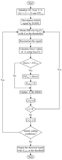
Figure 6.
Flowchart of the EEMD-IHHO.
4. Simulation and Analysis
4.1. Experimental Data and Evaluation Indicators
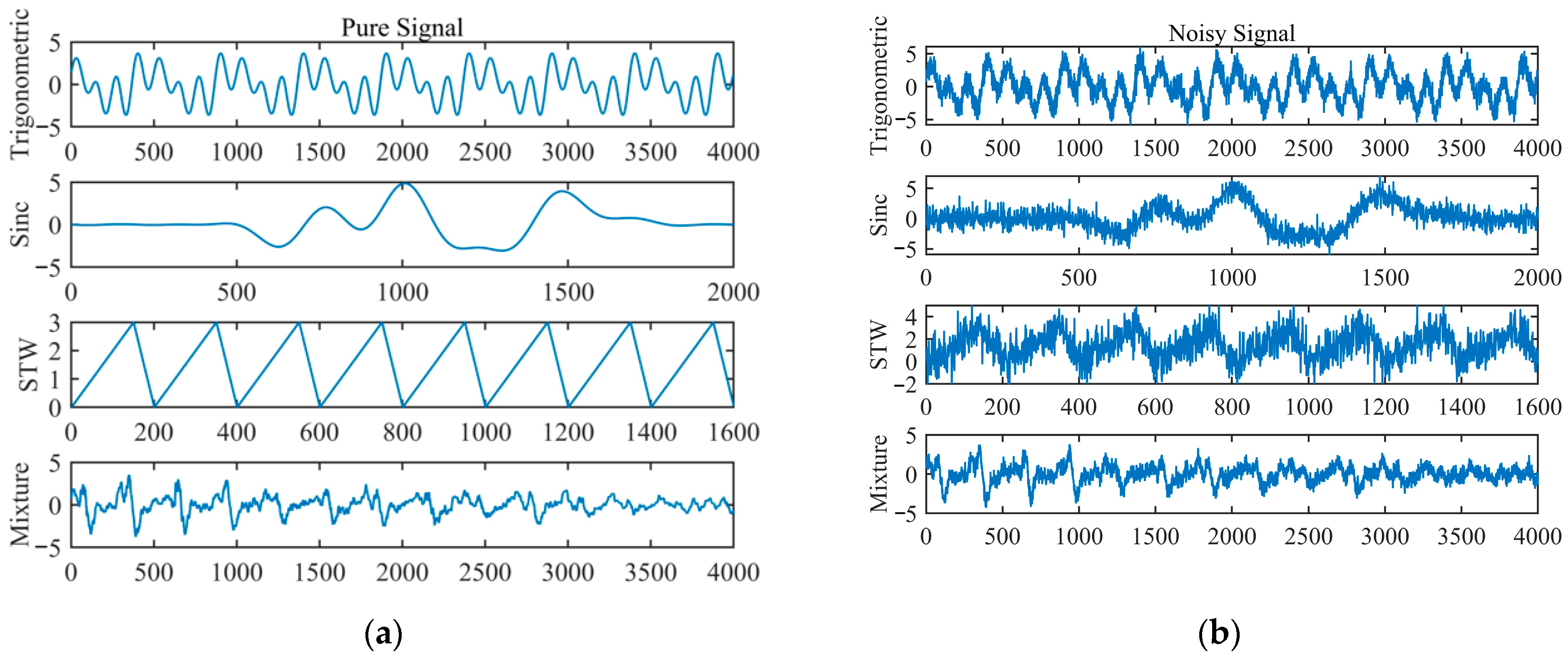
The simulation used the MATLAB2021 software platform based on the Windows 10 system environment. The denoising process of four types of signals was simulated to verify the effectiveness and superiority of the proposed method. The four types of signals are trigonometric function signal, sinc signal, sawtooth wave signal, and mixed signal. The first three pure signals were synthesized by the corresponding functions, and the fourth pure signal was extracted from the signal toolbox of MATLAB2021. They were shown in Figure 7a. To simulate the noise signal, white gaussian noise was added to the four signals, as shown in Figure 7b. By comparing the two images, it can be found that most of the features of the pure signal were drowned in noise. MSE and SNR were used to evaluate the reduction degree of the denoised signal. The calculation formulas of these two evaluation indicators were Equations (25) and (26).
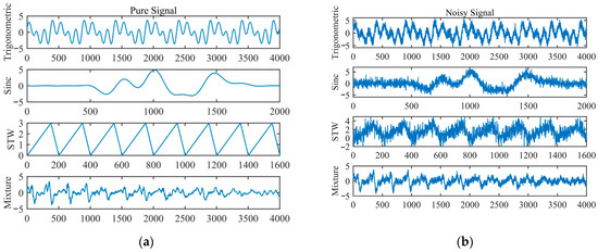
Figure 7.
(a) Waveforms of pure signals. (b) Waveforms of noisy signals.
4.2. Comparative Analysis
In order to fully verify the superiority of the proposed method, the denoising performance was compared with other four methods in this section. The four methods were traditional EEMD denoising, EEMD-HHO denoising, EEMD-particle swarm optimization (PSO) denoising, and the denoising method based on EEMD and grey theory mentioned in literature [32]. The parameter settings of each denoising scheme were given here:
- (1)
- EEMD denoising: Set the total number of added noise , the ratio of the standard deviation of the added noise to the original noisy signal .
- (2)
- EEMD-PSO denoising: Set the total number of added noise , ratio of the standard deviation of the added noise to the original noisy signal , number of particles , particle maximum speed , and maximum iterations number . Self-learning factor , group-learning factor , and inertia weight [33].
- (3)
- EEMD-HHO denoising and EEMD-IHHO denoising: Set the total number of noise added , the ratio of the standard deviation of the added noise to the original noisy signal , the maximum number of iterations in HHO , and the total number of eagles in the population . In EEMD-IHHO denoising, the escape energy was updated by Equation (25). Where was equal to 5.
- (4)
- EEMD-Grey denoising: Set the total number of added noise , the ratio of the standard deviation of the added noise to the original noisy signal , the resolution coefficient , and the weight coefficient .
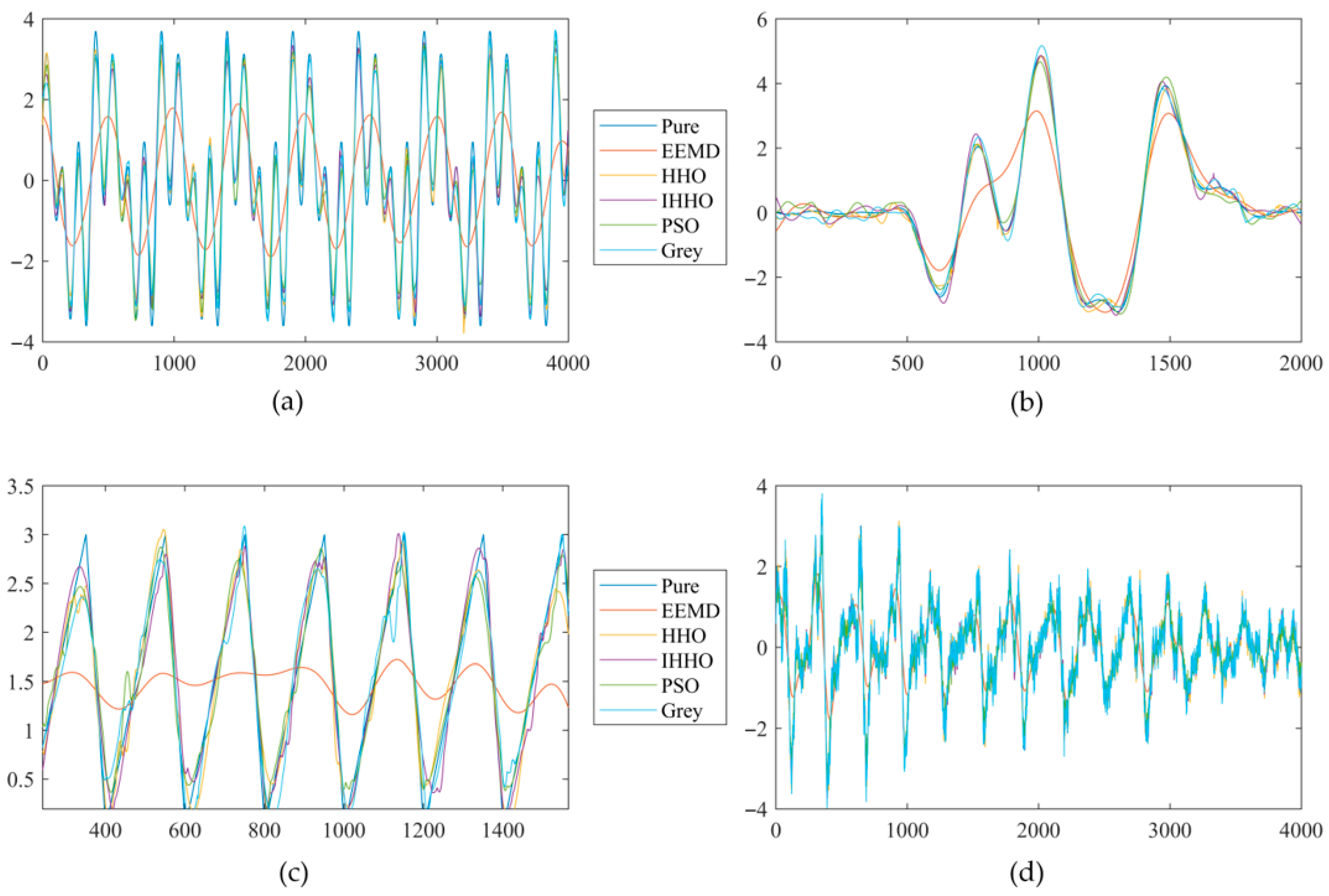
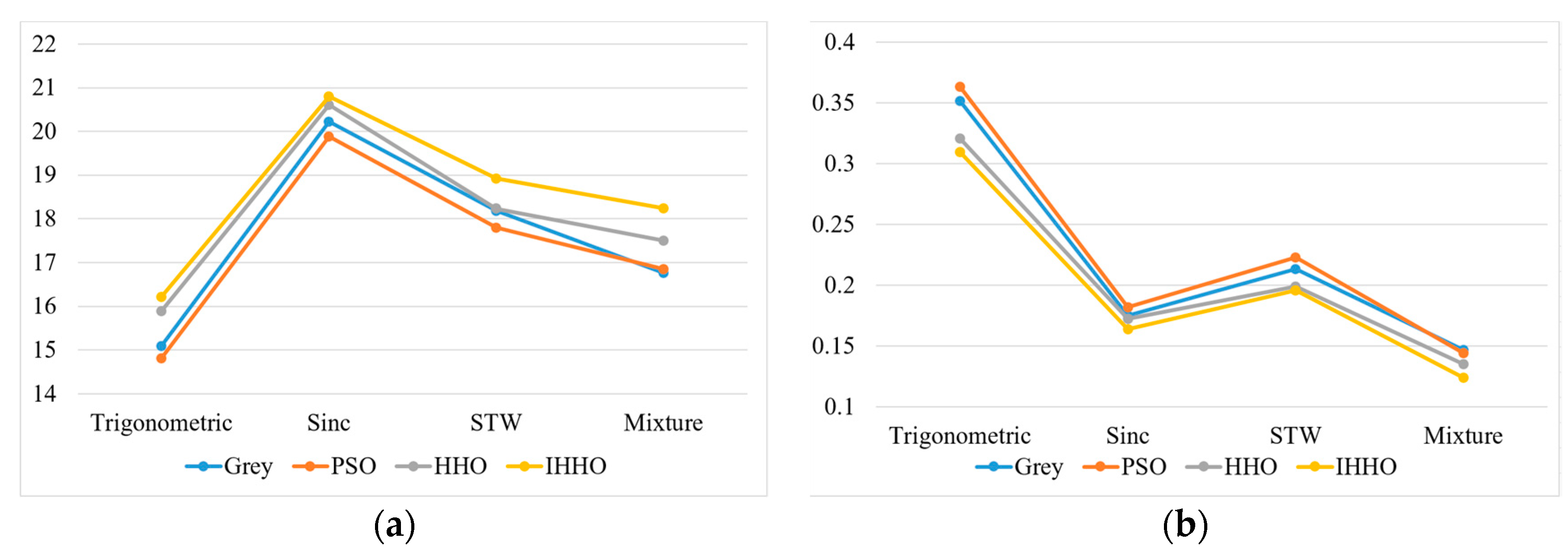
The signal waveform after denoising from the five algorithms was shown in Figure 8. As can be seen from Figure 8 that EEMD denoising was less effective, because the reconstructed signal was significantly different in waveform from the pure signal. In contrast, the signals processed by the other four schemes have high consistency with the pure signal. Its noise component was significantly reduced. After applying different methods of denoising to different types of signals, the evaluation indicators were calculated for each reconstructed signal, as shown in Table 1. The line graph was drawn, as shown in Figure 9. The proposed EEMD-IHHO denoising method had the smallest MSE. This proved that the signal denoised by this method had the least difference from the pure signal. The SNR was the largest, which proves that the signal obtained by this method had the largest proportion of the useful signal. Therefore, the denoising effect was the best. Specifically, compared with EEMD denoising, EEMD-PSO denoising, EEMD-HHO denoising, and EEMD-Grey denoising, the SNR of this method was increased by 70.9%, 6.7%, 2.6%, and 10.53% on average, respectively; and the MSE was decreased by 67.6%, 12.7%, 4.5%, and 5.42% on average, respectively.
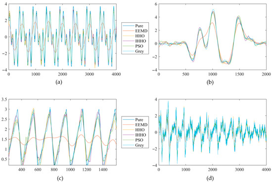
Figure 8.
Processing results of five denoising methods. (a) Trigonometric function signal. (b) Sinc signal. (c) Sawtooth wave signal. (d) Mixed signal.

Table 1.
(a) SNR of different denoising methods, (b) MSE of different denoising methods.
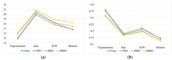
Figure 9.
(a) Signal-to-noise ratio line chart. (b) Mean squared error line chart.
To compare the denoising effect of the algorithm in different intensity noise environments, taking the mixed signal as an example, 0 dB, 5 dB, 10 dB, and 15 dB white gaussian noise were added respectively. The SNR and MSE of the denoised signal were shown in Table 2. As can be seen from Table 2, compared with EEMD denoising, EEMD-PSO denoising, EEMD-HHO denoising, and EEMD-Grey denoising, the SNR of this method was improved by 74.62%, 37.70%, 5.24%, and 39.72% on average, and by 76.86%, 43.52%, 13.79%, and 45.93% at the maximum. MSE was reduced by 77.38%, 53.10%, 9.88%, and 54.67% on average, and by 81.68%, 61.86%, 26.49%, and 62.63% at maximum. Meanwhile, it can be seen from Table 1 and Table 2 that for mixed signals with input SNR of 30 dB, the denoising performance of the five denoising algorithms was better than that when the input SNR was 15 dB. The SNR and MSE were significantly improved after denoising. It showed that with the weakening of the external noise signal, the recovery degree of the original signal was gradually enhanced by the denoising algorithm.
Table 2.
(a) SNR of different noise environments, (b) MSE of different noise environments.
5. Industrial Application
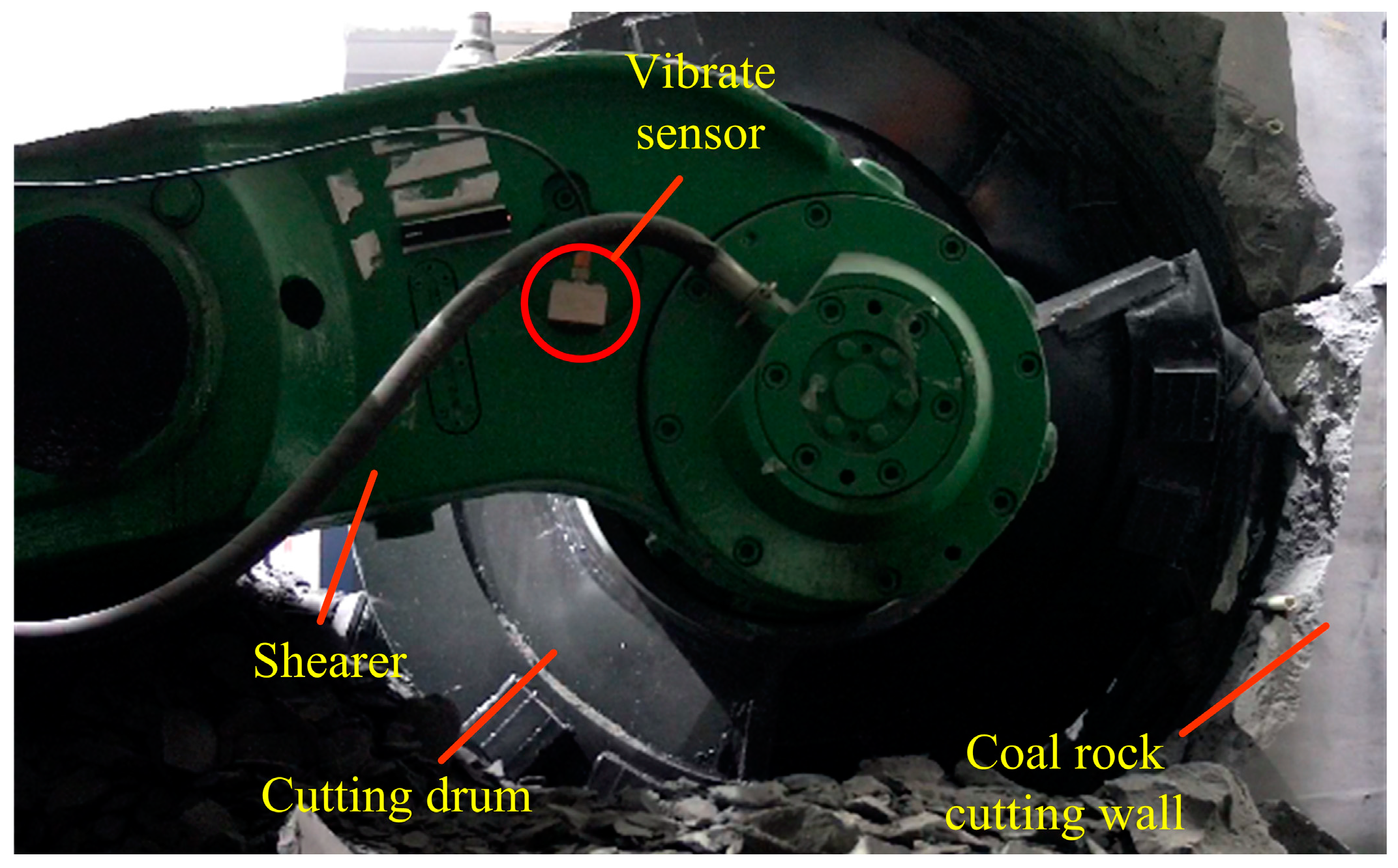
In order to verify the practicability of the proposed denoising method of mechanical vibration signal based on EEMD-IHHO, it was applied to the coal shearer working state diagnosis system. The project team developed a shearer working status diagnosis system based on vibration signals. The working state of the shearer can be divided into four typical working conditions: no-load, coal cutting, rock cutting, and coal and rock interlayer cutting. Firstly, the collected vibration signal is transmitted to the signal processing module through the signal transmission module. The signal processing module converts the vibration signal into a feature vector which can be used to identify the cutting state of coal and rock. The state recognition unit matches the feature vectors with the typical working condition template library. The cutting state identification of coal and rock and decision level fusion of each identification result are completed to obtain the final cutting state of coal and rock of shearer. On the other hand, when the meshing surface of the gear in the reduction box of the shearer contacts, the impulse force response will appear [34]. The vibration signal directly collected by the sensor is preprocessed by the signal processing related method. Then, using spectrum analysis technology, the corresponding characteristic frequency is diagnosed, and the frequency is judged to be abnormal. The frequency can determine the running state and whether there is a fault or not. The vibration signal was collected by an industrial-grade acceleration sensor with a sampling frequency of 4000 HZ. According to the Nyquist sampling theorem, the frequency of the collected signal is 0–2000 Hz. It was mounted on the rocker arm of the shearer facing the sample cutting. The arrangement of the shearer and sensors was shown in Figure 10. However, the vibration signals collected in the field are very complex and contain a lot of background noise. It not only includes the vibration signal generated by cutting coal seam and gear meshing, but also includes the vibration signal of the cutting motor, traction motor, and scraper conveyor. Therefore, before diagnosing and recognizing the working state of shearer, it needs to be denoised. The vibration signals of rocker arms of 20,000 shearers were collected on site, converted into WAV format, and imported into MATLAB. The proposed algorithm was used for denoising, and then the time domain and frequency domain analysis of the signal before and after denoising were carried out. The parameters of the algorithm were set as follows: set the total number of noise added , the ratio of the standard deviation of the added noise to the original noisy signal , the maximum number of iterations in HHO , the total number of eagles in the population . The escape energy was updated by Equation (25), where was equal to 5. The effectiveness of the proposed algorithm for denoising practical engineering signals was verified.
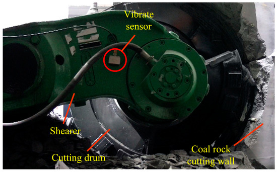
Figure 10.
Experimental site equipment arrangement.
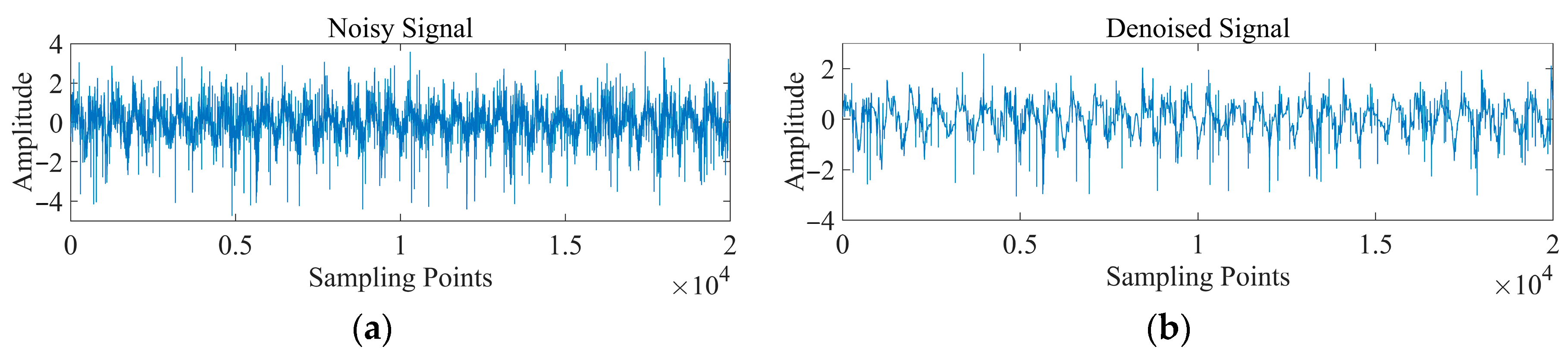
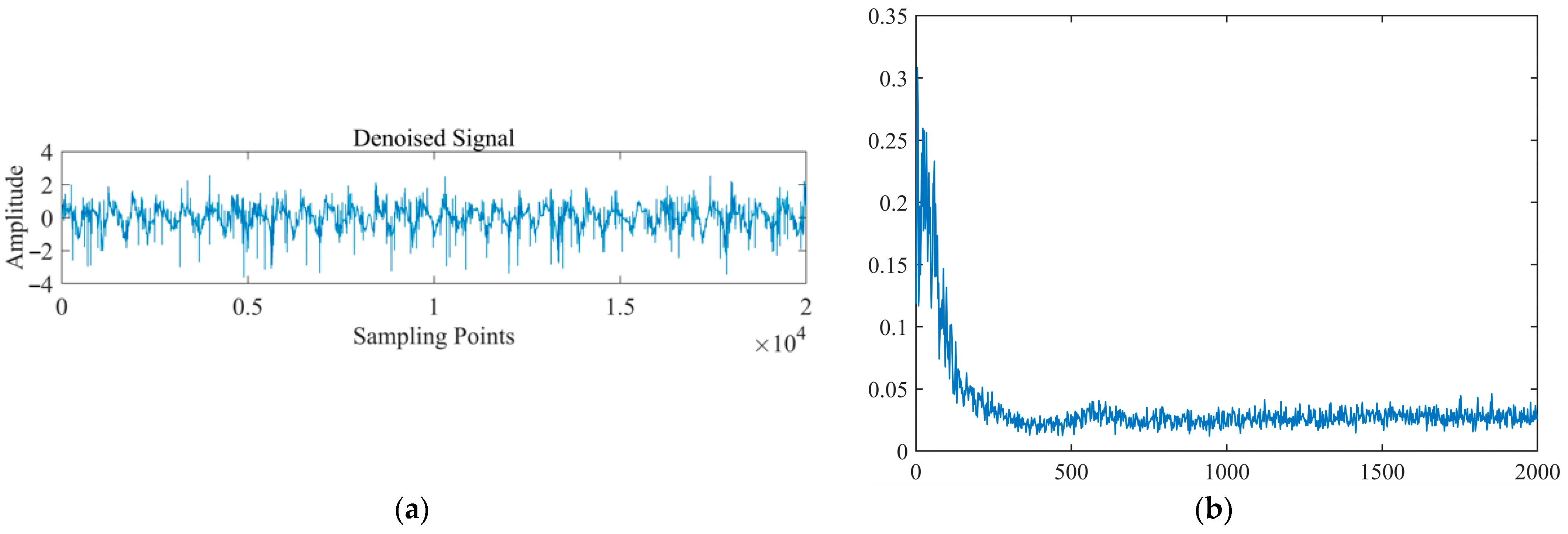
Figure 11a showed the time-domain waveform of the actual vibration signal collected. The signal was processed by the proposed denoising method, and then the time-domain waveform was shown in Figure 11b. Comparing Figure 11a,b, it can be found that the amplitude of the noisy signal was large and the waveform was dense. However, the denoising signal had smaller amplitude, sparse waveform, and less burr. The noise was largely eliminated, resulting in reduced signal components and amplitudes. The FFT was performed on the vibration signal before and after denoising, and the frequency spectrum was shown in Figure 12.
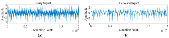
Figure 11.
(a) Time domain diagram of noisy signal. (b) Time domain diagram of denoised signal.

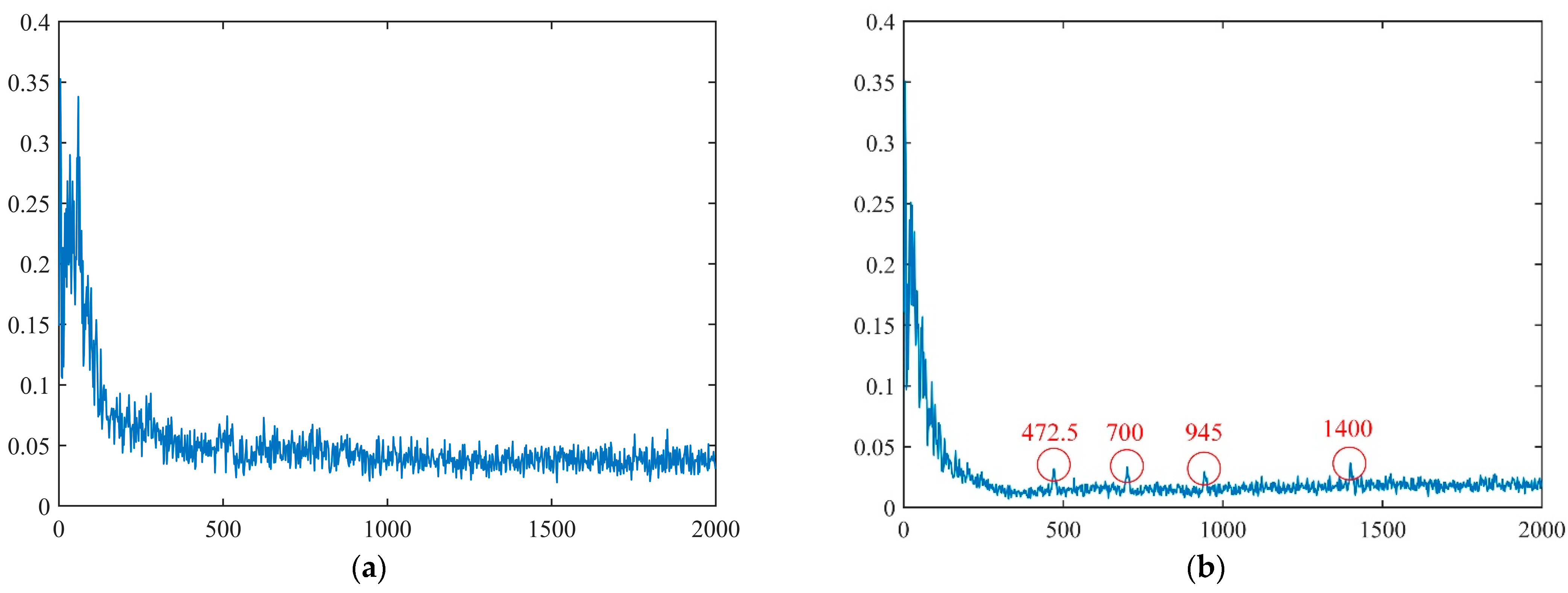
Figure 12.
(a) Spectrogram of noisy signal. (b) Spectrogram of denoised signal.
It can be seen from Figure 12a that there were many spurs in the full frequency domain of the noise signal. The high-frequency part was disordered and the characteristic frequencies were submerged in it. During the working process, the gear meshing in the reduction box of the shearer will produce a vibration signal with frequencies of 472.5 Hz and 700 Hz. The frequency in the fault state is an integer multiple of the gear engagement frequency. In other words, within 0–2000 Hz, the characteristic frequency of fault diagnosis is 472.5 Hz, 700 Hz, 945 Hz, and 1400 Hz [35]. It can be seen from Figure 12b that the spectral pattern of the denoised signal had less burr and a stable trend, and the overall amplitude had decreased. In addition, there were significant peaks around several key characteristic frequencies. Therefore, the denoised signal will be more suitable for the identification of the working state of the shearer. In order to further highlight the advantages of the proposed algorithm for actual engineering signal denoising, it is compared with the traditional EEMD denoising. The time domain diagram and frequency domain diagram of the signal after denoising were shown in Figure 13. By comparing the time domain Figure 11a and frequency domain Figure 12a of the original signal, it can be seen that the traditional EEMD method had a certain denoising effect. However, compared with Figure 11b in the time domain and Figure 12b in the frequency domain after denoising by the proposed algorithm, it can be found that the signal still contains more burrs in the time domain. In the frequency domain, although the amplitude decreases and the frequency component became sparse, there was no significant peak near several key characteristic frequencies. It showed that, compared with the proposed algorithm, the traditional EEMD has a limited denoising effect.
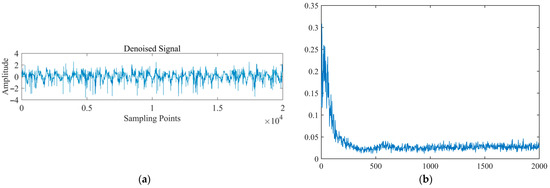
Figure 13.
(a) Time domain diagram after EEMD denoising. (b) Spectrogram of after EEMD denoising.
6. Conclusions and Future Work
In order to remove the noise in mechanical vibration signals, a new noise elimination method for coalcutter vibration signal based on EEMD and IHHO is proposed. Based on the original HHO, an exponential function based on the natural logarithm is used to determine the trend line of escape energy, and the escape energy is improved. IHHO is introduced to determine the threshold of EEMD denoising. According to the signal independence theory, the fitness function is established to evaluate the threshold. The simulation results show that, compared with the other four denoising algorithms, the proposed algorithm can always obtain the largest SNR and the smallest MSE after denoising signals. It shows that this method has an obvious advantage in denoising. Finally, it is applied to the processing of shearer vibration signals. By comparing the time domain and spectrum before and after denoising, the noise component is obviously reduced. Several key characteristic frequency peaks are displayed, which is beneficial to the identification of the working state of shearer. The practical application proves the effectiveness of the method.
However, there are some drawbacks to this approach. On the one hand, EEMD processing requires tens or even hundreds of EMDs, while IHHO requires hundreds of iterations. Therefore, it is difficult to reduce the time consumed by the whole denoising process. On the other hand, some parameters are determined according to previous experience without strict derivation. Improvements to code execution efficiency and parameter determination will be made in the future.
Author Contributions
J.X. and C.R. contributed the new method; C.R., Y.L. and X.C. designed the simulations and experiments; Y.L. and X.C. performed the experiments; J.X. wrote the paper. All authors have read and agreed to the published version of the manuscript.
Funding
This research was funded by the National Natural Science Foundation of China (No. 51905229), Natural Science Foundation of Jiangsu Province (No. BK20190968), China Postdoctoral Science Foundation (No. 2019M661975), and Marine Equipment and Technology Institute of Jiangsu University of Science and Technology (HZ20220001, HZ20220009 and HZ20220013). And the APC was funded by Marine Equipment and Technology Institute of Jiangsu University of Science and Technology (HZ20220001 and HZ20220009).
Institutional Review Board Statement
Not applicable.
Informed Consent Statement
Not applicable.
Data Availability Statement
Not applicable.
Acknowledgments
The author thanks the Jiangsu Province and Education ministry Co-sponsored Collaborative Innovation Center of Intelligent Mining Equipment and all the staff for their experimental support.
Conflicts of Interest
The authors declare no conflict of interest.
References
- Wang, F.; Mine, D.C. Discussion on the implementation scheme of unmanned fully mechanized mining face. Shaanxi Coal 2019, 38, 67–71+181. [Google Scholar]
- Wei, D.; Wang, Z.B.; Si, L.; Tan, C.; Lu, X.L. Online shearer-onboard personnel detection method for the intelligent fully mechanized mining face. Proc. Inst. Mech. Eng. Part C J. Mech. Eng. Sci. 2022, 236, 3058–3072. [Google Scholar] [CrossRef]
- Zhao, T.Y.; Jiang, L.P.; Pan, H.G.; Yang, J.; Kitipornchai, S. Coupled free vibration of a functionally graded pre-twisted blade-shaft system reinforced with graphene nanoplatelets. Compos. Struct. 2020, 16, 113362. [Google Scholar] [CrossRef]
- Si, L.; Wang, Z.B.; Tan, C.; Liu, X.H.; Xu, X.H. A feature extraction method for shearer cutting pattern recognition based on improved local mean decomposition and multi-scale fuzzy entropy. Curr. Sci. 2017, 112, 2243–2252. [Google Scholar] [CrossRef]
- Li, C.P.; Peng, T.H.; Zhu, Y.M. A Cutting Pattern Recognition Method for Shearers Based on ICEEMDAN and Improved Grey Wolf Optimizer Algorithm-Optimized SVM. Appl. Sci. 2021, 11, 9081. [Google Scholar] [CrossRef]
- Zhao, T.Y.; Ma, Y.; Zhang, H.Y.; Pan, H.G.; Cai, Y. Free vibration analysis of a rotating graphene nanoplatelet reinforced pre-twist blade-disk assembly with a setting angle. Appl. Math. Model. 2021, 93, 578–596. [Google Scholar] [CrossRef]
- Li, Z.X.; Jiang, Y.; Wang, X.P.; Peng, Z. Multi-mode separation and nonlinear feature extraction of hybrid gear failures in coal cutters using adaptive nonstationary vibration analysis. Nonlinear Dyn. 2016, 84, 295–310. [Google Scholar] [CrossRef]
- Velasco-Forero, S.; Pages, R.; Angulo, J. Learnable Empirical Mode Decomposition based on Mathematical Morphology. Siam J. Imaging Sci. 2022, 15, 23–44. [Google Scholar] [CrossRef]
- Barbosh, M.; Singh, P.; Sadhu, A. Empirical mode decomposition and its variants: A review with applications in structural health monitoring. Smart Mater. Struct. 2020, 29, 093001. [Google Scholar] [CrossRef]
- Hao, H.B.W.; Yu, F.H.; Li, Q.L. Soil Temperature Prediction Using Convolutional Neural Network Based on Ensemble Empirical Mode Decomposition. IEEE Access 2021, 9, 4084–4096. [Google Scholar] [CrossRef]
- Liu, X.P.; Zhang, Y.Q.; Zhang, Q.C. Comparison of EEMD-ARIMA, EEMD-BP and EEMD-SVM algorithms for predicting the hourly urban water consumption. J. Hydroinform. 2022, 24, 535–558. [Google Scholar] [CrossRef]
- Chan, J.; Ma, H.; Saha, T.; Ekanayake, C. Self-adaptive partial discharge signal de-noising based on ensemble empirical mode decomposition and automatic morphological thresholding. IEEE Trans. Dielectr. Electr. Insul. 2014, 21, 294–303. [Google Scholar] [CrossRef]
- Li, J.; Tong, Y.; Guan, L.; Wu, S.; Li, D. A uv-visible absorption spectrum denoising method based on eemd and an improved universal threshold filter. RSC Adv. 2018, 8, 8558–8568. [Google Scholar] [CrossRef] [PubMed]
- Cai, J.H.; Xiao, Y.L. Impulse interference processing for mt data based on a new adaptive wavelet threshold de-noising method. Arab. J. Geosci. 2017, 10, 1–10. [Google Scholar]
- Nguyen, P.; Kim, J.-M. Adaptive ecg denoising using genetic algorithm-based thresholding and ensemble empirical mode decomposition. Inf. Sci. 2016, 373, 499–511. [Google Scholar] [CrossRef]
- Jain, S.; Bajaj, V.; Kumar, A. Effective de-noising of ecg by optimised adaptive thresholding on noisy modes. IET Sci. Meas. Technol. 2018, 12, 640–644. [Google Scholar] [CrossRef]
- Zhang, Q.; Wang, T.; Zhao, J.; Liu, J.; Wang, Y.; Zhang, J.; Qiao, L.; Zhang, M. A dual-adaptive denoising algorithm for brillouin optical time domain analysis sensor. IEEE Sens. J. 2021, 21, 22712–22719. [Google Scholar] [CrossRef]
- Zhang, L.Y.; Ren, Z.C.; Liu, T.; Tang, J.Y. Improved Artificial Bee Colony Algorithm Based on Harris Hawks Optimization. J. Internet Technol. 2022, 23, 379–389. [Google Scholar] [CrossRef]
- Bednarz, J.C. Cooperative hunting harris’ hawks (parabuteo unicinctus). Science 1988, 239, 1525–1527. [Google Scholar] [CrossRef]
- Hussien, A.G.; Abualigah, L.; Abu Zitar, R.; Hashim, F.A.; Amin, M.; Saber, A.; Almotairi, K.H.; Gandomi, A.H. Recent advances in harris hawks optimization: A comparative study and applications. Electronics 2022, 11, 1919. [Google Scholar] [CrossRef]
- Qu, C.W.; He, W.; Peng, X.G.; Peng, X.N. Harris hawks optimization with information exchange. Appl. Math. Model. 2020, 84, 52–75. [Google Scholar] [CrossRef]
- Kamboj, V.K.; Nandi, A.; Bhadoria, A.; Sehgal, S. An intensify harris hawks optimizer for numerical and engineering optimization problems. Appl. Soft Comput. 2020, 89, 106018. [Google Scholar] [CrossRef]
- Shao, K.; Fu, W.; Tan, J.; Wang, K. Coordinated approach fusing time-shift multiscale dispersion entropy and vibrational harris hawks optimization-based svm for fault diagnosis of rolling bearing. Measurement 2021, 173, 108580. [Google Scholar] [CrossRef]
- Hussain, K.; Zhu, W.; Salleh, M.N.M. Long-term memory harris hawk optimization for high dimensional and optimal power flow problems. IEEE Access 2019, 7, 147596–147616. [Google Scholar] [CrossRef]
- Donoho, D.L.; Johnstone, I.M. Ideal spatial adaptation by wavelet shrinkage. Biometrika 1994, 81, 425–455. [Google Scholar] [CrossRef]
- Xie, B.; Xiong, Z.Q.; Wang, Z.J.; Zhang, L.J.; Zhang, D.Z.; Li, F.S. Gamma spectrum denoising method based on improved wavelet threshold. Nucl. Eng. Technol. 2020, 52, 1771–1776. [Google Scholar] [CrossRef]
- Fan, S.S.; Wang, X.H.; Zhang, Y.H. Study on PD detection for GIS based on autocorrelation coefficient and similar Wavelet soft threshold. Clust. Comput. J. Netw. Softw. Tools Appl. 2019, 22, 6755–6766. [Google Scholar] [CrossRef]
- Sihwail, R.; Omar, K.; Ariffin, K.A.Z.; Tubishat, M. Improved harris hawks optimization using elite opposition-based learning and novel search mechanism for feature selection. IEEE Access 2020, 8, 121127–121145. [Google Scholar] [CrossRef]
- Heidari, A.A.; Mirjalili, S.; Faris, H.; Aljarah, I.; Mafarja, M.; Chen, H. Harris hawks optimization: Algorithm and applications. Future Gener. Comput. Syst. 2019, 97, 849–872. [Google Scholar] [CrossRef]
- Ma, B.Z.; Zhang, T.Q. Single-channel blind source separation for vibration signals based on TVF-EMD and improved SCA. IET Signal Process. 2020, 14, 259–268. [Google Scholar] [CrossRef]
- Lou, S.T.; Zhang, X.D. Fuzzy-based learning rate determination for blind source separation. IEEE Trans. Fuzzy Syst. 2003, 11, 375–383. [Google Scholar]
- Jia, Y.C.; Li, G.L.; Dong, X.; He, K. A novel denoising method for vibration signal of hob spindle based on EEMD and grey theory. Measurement 2021, 169, 108490. [Google Scholar] [CrossRef]
- Hassan, F.; Ab Rahim, L.; Mahmood, A.K.; Abed, S.A. A Hybrid Particle Swarm Optimization-Based Wavelet Threshold Denoising Algorithm for Acoustic Emission Signals. Symmetry 2022, 14, 1253. [Google Scholar] [CrossRef]
- Meng, Z.; Shi, G.; Wang, F. Vibration response and fault characteristics analysis of gear based on time-varying mesh stiffness. Mech. Mach. Theory 2020, 148, 103786. [Google Scholar] [CrossRef]
- Mao, Q.; Zhang, Y.; Zhang, X.; Zhang, G.; Fan, H.; Mushayi, K. Accurate fault location method of the mechanical transmission system of shearer ranging arm. IEEE Access 2020, 8, 202260–202273. [Google Scholar] [CrossRef]


Publisher’s Note: MDPI stays neutral with regard to jurisdictional claims in published maps and institutional affiliations. |
© 2022 by the authors. Licensee MDPI, Basel, Switzerland. This article is an open access article distributed under the terms and conditions of the Creative Commons Attribution (CC BY) license (https://creativecommons.org/licenses/by/4.0/).