Interior Distance Ratio to a Regular Shape for Fast Shape Recognition

Abstract

A fast shape recognition method based on regular graphic is proposed in this paper. It is the Interior Distance Ratio to a regular Shape (minimum bounding rectangle (MBR) or minimum circumscribed circle (MCC)) (SIDR). Regular shapes themselves have either axisymmetric or origin symmetry, which gives them regularity. Shape, as a feature of an object, plays a significant role in computer vision and image analysis. The shape descriptor is widely used to compute remarkable features of the visual image, especially in image understanding and analysis. SIDR is a new remarkable feature of the shape, which is the distribution of the interior distance between the shape contour points and its minimum bounding rectangle or minimum circumscribed circle. It can provide more effective performance support for practical application fields of computer vision, such as object detection and recognition. The minimum bounding rectangle or minimum circumscribed circle can change according to the change in a shape’s position, scale and direction, which is extremely suitable for describing a shape that has deformation. In addition, the rectangularity and circularity derived from them also have the potential peculiarity to describe the shape feature. Therefore, this paper uses the interior distance ratio of the shape to represent the shape feature. First, the minimum bounding rectangle or minimum circumscribed circle of the shape is selected according to the rectangularity and circularity of the shape. Then, the interior distance proportional distribution from the shape contour point to the minimum bounding rectangle or minimum circumscribed circle is obtained. Finally, a histogram is used to represent the distribution feature, and shape matching and recognition are carried out. A self-built dataset and three international generic datasets are used to verify the validity of the method. The performance exhibits the sophisticated property (accuracy and matching speed) of the proposed method. It is worth mentioning that this simple method has a recognition rate of close to 100% on the self-built dataset and has achieved excellent results for other datasets compared with some international state-of-the-art methods.

1. Introduction

Regular shapes (rectangle, circle, equilateral triangle, etc.) [1,2] have their own characteristics of symmetry in geometry. They have stable features, such as symmetry, angular equality, parallelization, etc. They are closed graphics, which can be used to restrict a certain object in a certain area. In particular, the minimum bounding rectangle and the minimum circumscribed circle of the object can reflect the overall position, direction, size and other features of the object. Hence, it is significant to represent and embody the features of an object inside these regular graphics using the shape feature.

The shape feature is one of the important research bunches in image analysis. It is generally used in computer vision and image understanding, visual computing and target recognition. When the target area occupies a small part of the whole image area or the target texture feature is not clear, especially in remote sensing targets, the computer system can successfully understand and identify the target through the shape features. It is worth mentioning that deep learning methods with a lot of training can also detect and recognize the targets, but large shape datasets are difficult to obtain. At this time, shape descriptors are a meaningful tool for computer to analyze the target.

Many shape descriptors have been published [3,4,5,6]. Shape descriptors are widely used to obtain shape features of a target in an image, such as FD (Fourier descriptor) [7], CCD (centroid contour distance) [8], FD-CCD (FD based CCD) [7], FPD (farthest point distance) [9], WD (wavelet descriptor) [10], SC (shape context) [11], BPS (Bone Point Segment) [12] and FD-IDBS (FD-Bone point Segmentation using Inner Distance) [13]. There are some modified descriptors of the FMSCCD (Fourier descriptor based on multi-scale centroid distance) [14], IDSC (shape context based on inner distance) [15], DIR (distance interior ratio) [16] and ASD&CCD (angular scale descriptor based on distance from centroid) [17].

The basic ability to evaluate a shape descriptor is mainly enabled by the invariances of translation, rotation and scaling of the shape, such as [18,19,20]. The minimum bounding rectangle and minimum circumscribed circle of a shape are one-to-one related to the shape. If the shape has different positions, angles and sizes, the minimum bounding rectangle and minimum circumscribed circle will change accordingly. Therefore, its minimum bounding rectangle and minimum circumscribed circle can represent strong robust feature information of the shape. In other words, the minimum bounding rectangle and minimum circumscribed circle have translation invariance, rotation invariance and scale invariance to the shape itself. Using the minimum bounding rectangle and minimum circumscribed circle to denote the shape has potential advantages, such as strong descriptive ability and robustness.

In summation, most of the easy-to-understand features and simple calculation principles for a descriptor can only represent the rough features of the shape, but cannot distinguish dissimilar features caused by deformation. The method proposed in this paper uses a simple feature structure—the interior distance ratio to the regular graphic—to give shape descriptors a sophisticated recognition ability, which has a robust performance. The author’s innovation points and contribution includes four aspects.

(1)

The rectangularity and circularity of shape are proposed selectively to judge the initial feature of the shape;

(2)

A new shape feature based on the vertical interior distance to the minimum bounding rectangle is proposed to describe some shapes that are more like a rectangle;

(3)

A new shape feature based on the diameter interior distance to the minimum circumscribed circle is proposed to describe some shapes that are more like a circle;

(4)

A new and more effective shape recognition method is proposed, which provides greater possibilities for the practical application of object detection and recognition, including faster speed and higher recognition accuracy.

2. Preliminary

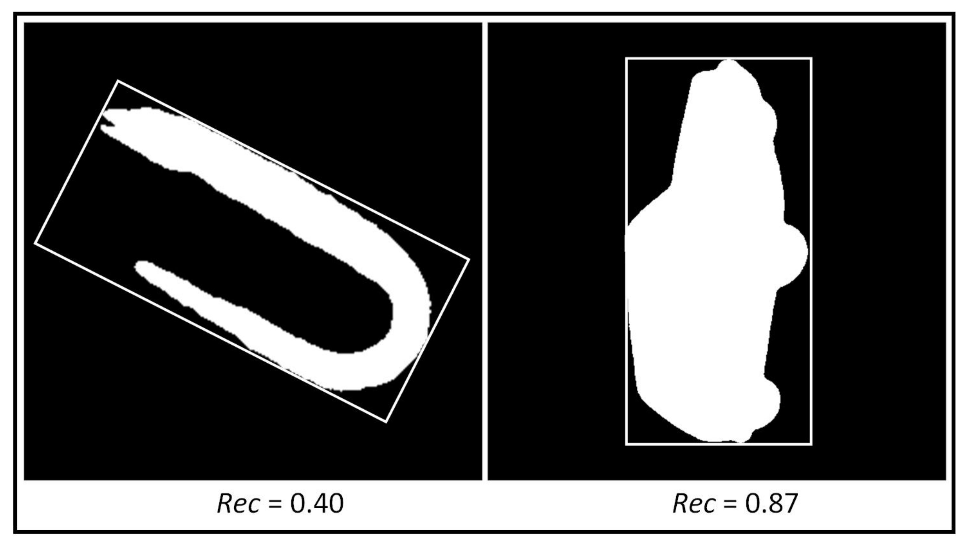
2.1. Rectangularity

The rectangularity [21,22] is defined as the ratio of the target area to the minimum bounding rectangle area. In this paper, the target represents the region of the shape.

2.1.1. The Acquisition Strategy of Minimum Bounding Rectangle

The minimum bounding rectangle refers to the maximum rectangular range of a number of two-dimensional shapes (such as points, lines and polygons) represented by two-dimensional coordinates; that is, the rectangle whose boundary is determined by the maximum abscissa, minimum abscissa, maximum ordinate and minimum ordinate in each vertex of a given two-dimensional shape. Such a rectangle contains a given two-dimensional shape and has a minimum area, etc.

There are two types of minimum bounding rectangles for general graphic: the minimum area bounding rectangle and the minimum perimeter bounding rectangle. In this article, the minimum area bounding rectangle is used. The following steps are the key to calculating the bounding rectangle.

• Find the four points $x_{minp},x_{maxp},y_{minp},y_{maxp}$ with the largest and smallest coordinates of UDLR(Up, Down, Left, Right);
• Four tangents can be constructed by these four points;
• If one (or two) lines coincide with one side, the area of the rectangle constructed by the four lines is calculated and defined as the current minimum area. Otherwise, the current minimum area is defined as infinity;
• Rotate the lines clockwise until one of them coincides with an edge of the polygon;
• Calculate the area of the new rectangle and compare it with the current minimum area. If it is less than that, update and save the area of the new rectangle as the minimum area;
• Repeat Step 4 and 5 until the angle of the line is rotated by more than 90°;
• Get the minimum bounding rectangle.

Figure 1 below exhibits some legends of the minimum bounding rectangle for the shape.

2.1.2. The Calculation Method of Rectangularity

In the actual calculation of this paper, the rectangularity is expressed as the ratio of the number of pixels ($N_{r}s$) occupied by the target shape to the number of pixels ($N_{r}r$) occupied by the smallest enclosing rectangle. The calculation equation of rectangularity is shown in Equation (1).

$$Rec=S_{r}s/S_{r}r=N_{r}s/N_{r}r$$

(1)

where, $S_{r}s$ represents the area of the shape and $S_{r}r$ represents the area of the minimum bounding rectangle.

2.2. Circularity

The circularity [22,23] is defined as the ratio of the target area to the minimum circumscribed circle area. In this paper, the target represents the region of the shape.

2.2.1. The Acquisition Strategy of Minimum Circumscribed Circle

The minimum circumscribed circle refers to the maximum circle range of a number of two-dimensional shapes (such as points, lines and polygons) represented by two-dimensional coordinates as the minimum circumscribed circle. Such a circle contains a given two-dimensional shape and has a minimum area, etc. In 2000, Wang Wei et al. proposed an accurate and fast least circumscribed circle algorithm (DFAA) [24]. The key steps of the algorithm are as follows.

• Find $P_1,P_2,P_3$ in the contour point set P;
• Use the above points to construct the circumscribed circle C;
• Query the point Q, which is the farthest point from the centre of C in the point set P. If Q is inside the C, the step terminates. Otherwise, carry out Step 4;
• For the points of $P_1,P_2,P_3$, and Q, construct the circumscribed circle D; it contains the above points. Then, go to Step 2. Until the minimum circumscribed circle is found;
• Output the minimum circumscribed circle.

Say it picks three points at random, $P_1\left(x_1,y_1\right),P_2\left(x_2,y_2\right),P_3\left(x_3,y_3\right)$. The calculation equation of the circumcircle is as shown in Equation (2).

$$r=\left(P_1{P}_2\right)/2,a=\left(x_1+x_2\right)/2,b=\left(y_1+y_2\right)/2$$

(2)

where r is the radius of the circumscribed circle, a is the abscissa of the centre of the circumscribed circle and b is the ordinate of the centre of the circumscribed circle.

Especially, when the triangle composed of three points $P_1\left(x_1,y_1\right),P_2\left(x_2,y_2\right),P_3\left(x_3,y_3\right)$ is a right-angle triangle or an obtuse triangle, the calculation equation of the circumscribed circle is as shown in Equation (3) or Equation (4), respectively.

$$r=\left(P_2{P}_3\right)/2,a=\left(x_2+x_3\right)/2,b=\left(y_2+y_3\right)/2$$

(3)

$$\begin{array}{cc}\hfill & r={\left({\left(x_1-a\right)}^2+{\left(y_1-b\right)}^2\right)}^{1/2}\hfill \\ \hfill & a=\frac{\left(\left({\left(x_1^2-x_2^2\right)}^2+{\left(y_1^2-y_2^2\right)}^2\right)\ast \left(y_2-y_3\right)\right)-\left(\left({\left(x_2^2-x_3^2\right)}^2+{\left(y_2^2-y_3^2\right)}^2\right)\ast \left(y_1-y_2\right)\right)}{\left(2\ast \left(x_1-x_2\right)\ast \left(y_2-y_3\right)-2\ast \left(x_2-x_3\right)\ast \left(y_1-y_2\right)\right)}\hfill \\ \hfill & b=\frac{\left(\left({\left(x_1^2-x_2^2\right)}^2+{\left(y_1^2-y_2^2\right)}^2\right)\ast \left(x_2-x_3\right)\right)-\left(\left({\left(x_2^2-x_3^2\right)}^2+{\left(y_2^2-y_3^2\right)}^2\right)\ast \left(x_1-x_2\right)\right)}{\left(2\ast \left(y_1-y_2\right)\ast \left(x_2-x_3\right)-2\ast \left(y_2-y_3\right)\ast \left(x_1-x_2\right)\right)}\hfill \end{array}$$

(4)

Figure 2 below exhibits some legends of minimum circularity circle for shapes.

2.2.2. The Calculation Method of Circularity

In the actual calculation of this paper, the circularity is expressed as the ratio of the number of pixels ($N_{c}s$) occupied by the target shape to the number of pixels ($N_{c}c$) occupied by the smallest enclosing rectangle. The calculation equation of rectangularity is shown in Equation (5).

$$Cir=S_{c}s/S_{c}c=N_{c}s/N_{c}c$$

(5)

where $S_{c}s$ represents the area of the shape and $S_{c}c$ represents the area of the minimum circumscribed circle.

2.3. The Effectiveness of Rectangularity and Circularity

The minimum bounding rectangle and minimum circumscribed circle possess the properties of position, size and direction, which can enhance the performance of shape features. The rectangularity and circularity also mirror the shape feature to a large extent. For instance, the Centroid Contour Distance (CCD) [8] is a simple and classical shape descriptor. The sequence $p=p_1,p_2,p_3,\dots ,p_{\left(N_P\right)}$ is the contour sample points after sampling of the shape contour. The centroid contour points $P_c$ of the shape are calculated using Equation (6) below.

$$P_c=1/N_P\sum _{i=1}^{N_P}{p}_i=\left(1/N_P\sum _{i=1}^{N_P}{x}_i,1/N_P\sum _{i=1}^{N_P}{y}_i\right)$$

(6)

where $N_P$ means the number of sampling points on the contour, $\left(x_i,y_i\right)$ is the $ith$ contour point $p_{\left(i\right)}$ of a shape. Then, the Euclidean distance between each contour point $p_i\left(x_i,y_i\right)$ and the centroid contour point $P_c\left(x_c,y_c\right)$ is calculated via Equation (7) below.

$$d_{ic}={\left({\left(x_i-x_c\right)}^2+{\left(y_i-y_c\right)}^2\right)}^{(1/2)}$$

(7)

Finally, the Euclidean distance $d_{i}c$ is normalized to obtain the centroid contour distance $d_{ccd}^i$, calculated using Equation (8).

$$d_{ccd}^i=\left(\frac{d_{ic}}{\left(1/N_P\right){\sum }_{j=1}^{N_P}{d}_{jc}}\right)/\sqrt{N_P}=d_{ic}\sqrt{N_P}/\sum _{j=1}^{NP}{d}_{jc},i=1,2,3,\dots N_P$$

(8)

The CCD feature is the sequence $d_{ccd}^{(m+i)}=d_{ccd}^{\left(m+i-N_P\right)}$. In order to match the invariance of the starting point, the distance between two shapes $s1$ and $s2$ is calculated using Equation (9) below.

$${dis}_{ccd}(s1,s2)=\underset{0\le m\le N_P}{min}{\left(\sum _{i=1}^{N_P}{\left(d_{ccd}^i-d^{m+i}{}_{ccd}\right)}^2\right)}^{\frac{1}{2}},m\in Z$$

(9)

where $d_{ccd}^{(m+i)}=d_{ccd}^{\left(m+i-N_P\right)}$. This distance is used for shape matching.

Some scholars proposed FD-CCD. The FD-CCD has performed a Fourier transform on the CCD and converted it to the frequency domain to obtain the more robust shape descriptor, as shown in Equation (10).

$$F_{ccd}\left(k\right)=1/N_P\left|\sum _{i=0}^{N_P-1}{d}_{ccd}^i{e}^{\left((-j2\pi ik)/N_P\right)}\right|,k=0,1,\dots ,N_P-1$$

(10)

The distance between the two shapes is also converted to the frequency domain, as shown in Equation (11).

$$di{s}_{f}c\left(s_1,s_2\right)=\sum _{k=0}^K\left|F_{ccd}^{\left(s_1\right)}\left(k\right)-F_{ccd}^{\left(s_2\right)}\left(k\right)\right|,0\le K\le N_P$$

(11)

where K is the number of characteristic coefficients in the frequency domain. In this paper, K = 100.

The CCD and FD-CCD descriptors all have invariance of translation due to their normalized Euclidean distance. Following the process of the matching structure above, they have invariance of rotation, but their experimental performance is very weak (low accuracy, low speed and high complexity).

Following in-depth study of CCD and FD-CCD, the author found that they have the same defects (distinguishing two shapes that have the same spatial relationship in contours). The modified CCD of FD-CCD is only slightly better in terms of anti-interference, but does not solve the defect. Meanwhile, in the two pairs of images shown in Figure 1 and Figure 2, although the naked eye can distinguish between them, neither of these two algorithms can easily tell them apart. Figure 3 and Figure 4 show CCD feature vector curves of the two pair of shapes.

It can be seen intuitively from Figure 3 and Figure 4 that the feature vectors of these two types of shapes are very similar. Figure 5 and Figure 6 show FD-CCD feature vector curves of the two pairs of shapes.

It can be seen analogously from Figure 5 and Figure 6 that the feature vectors of these two types of shapes are very similar, too. Based on the above analysis, the features of rectangularity and circularity are added to FD-CCD feature to form a new Syncretic Fourier Descriptor based on CCD (SFD-CCD), it can be defined as $F_{ccd}^{r}c$, which is expressed as Equation (12) below.

$$F_{ccd}^{rc}=\left\{\begin{array}{c}{F}_{ccd}+F_r,Rec\to 1\hfill \\ F_{ccd}+F_c,Cir\to 1\hfill \end{array}\right.$$

(12)

where $F_r$ and $F_c$ represent the rectangularity feature and circularity feature, respectively; $Rec\to 1$ means the shape is more like a rectangle; $Cir\to 1$ means the shape is more like a circle. Figure 7 and Figure 8 show SFD-CCD feature vector curves of the two pairs of shapes.

Although CCD and FD-CCD are simple and effective shape descriptors, they lose the robustness of shape descriptors in many cases. As shown in Figure 3, Figure 4, Figure 5 and Figure 6, they were unable to correctly distinguish between shapes. As for SFD-CCD descriptors with rectangularity and circularity features, it is obvious from Figure 7 and Figure 8 that they are different class shapes. At the same time, the above analysis and experiment reveal the validity of the features of rectangularity and circularity. It is worth mentioning that these two features have translation, scale and rotation invariance as well.

2.4. Interior Distance

Distance is an important mathematical variable used to describe shapes [25,26]. The distance we generally refer to is called Euclidean distance, which is the distance of a straight line. The interior distance [16,27] is the distance of the summation of portions on a line segment that are lying inside the polygon and the length of the line segment.

In this paper, we assume that the target area in the image is segmented and the pixel coordinates are known. The line segment can be defined as a set $P=\left\{P_1,P_2,\dots ,P_{N1}\right\}$, where $N1$ is the total number of uniformly selected pixels on the line segment and $P_i=\left(x_i,y_i\right)$ is the coordinate of the pixel i. The pixels of the target are defined as a set $S=\left\{S_1,S_2,\dots ,S_{N2}\right\}$, where $N2$ is the total number of target pixels. Let $\left(P_i,P_j\right)$ be a line segment connecting points $P_i\in P$ and $P_j\in P$, where $i\ne j$.

Let $D\left(P\right)=\left\{d_{1,2},d_{2,3},\dots ,d_{N-1,N}\right\}$ denote a set of pairwise interior distances among points in P, where $d_{ij}$ is the interior distance of $\left(P_i,P_j\right)$, where $P_i\in P$ and $P_j\in P$ where $P_i\ne P_j$. To compute $d_{ij}$, this work uses the method of intersection of line segment and shape to calculate the number of intersecting pixels, which can approximate and extract a pixel line segment of $\left(P_i,P_j\right)$; more clearly, it is $\left(P_i,P_j\right)\cap S$. Let $L\left(P_i,P_j\right)=\left\{l_1,l_2,\dots ,l_K\right\}$ be a set of K pixels on the pixel line segment. An example of a pixel line segment $L\left(P_i,P_j\right)$ is shown in Figure 9b. This work only considers binary images, assuming that the value $V\left(l_n\right)$ of every pixel $l_n$ is either one or zero. If the value of a pixel $V\left(l_n\right)$ equals one (dark pixels), then the pixel is lying inside the shape’s region; otherwise, it lies outside. Let $lc$ be the number of pixels $l_n$ for $1\le n·\le$ with $V\left(l_n\right)=1$. From Figure 9b, we have $l_c=8$. So, the interior distance $\left(l_c\right)$ of the line segment $P_i{P}_j$ is eight.

3. SIDR

In this section, the detailed procedure of the proposed method is explained in detail. Based on the above analysis of the effectiveness of rectangularity and circularity in describing shape features, this work proposes a syncretic shape signature based on the minimum bounding rectangle and minimum circumscribed circle using an interior distance ratio. First, the rectangularity and circularity of the shape are calculated. If the shape is closer to a rectangle (the rectangularity value of the shape is greater than the circularity value), the minimum bounding rectangle of the shape is calculated and the interior distance ratio between the contour points of the shape and the rectangle is calculated. If the shape is closer to a circle (the circularity value of the shape is greater than the rectangularity value of the shape), the minimum circumscribed circle of the shape is found and the interior distance ratio between the contour points of the shape and the circle is calculated. Then, the histogram of the interior distance ratio of all contour points is obtained. Finally, shape matching and recognition are carried out. The framework of the proposed method is shown in Figure 10. It contains six parts altogether, from input to output.

The shapes are different, so this paper selects the minimum bounding rectangle and the minimum circumscribed circle selectively for different shapes, in order to reduce the amount of calculation as much as possible during the calculation process, and then speed up the shape recognition. The specific selection strategy is presented.

3.1. The Similarity of the Shape to the Minimum Bounding Rectangle and the Minimum Circumscribed Circle

Assuming that the rectangularity of the shape is $rec$ and the circularity of the shape is $cir$, if $rec>cir$, the minimum bounding rectangle is selected to calculate the corresponding proportion of internal distance. Otherwise, select the minimum circumscribed circle to find the corresponding interior distance ratio.

3.2. Interior Distance Ratio to Minimum Bounding Rectangle of a Shape

If the rectangularity of a shape is greater than the circularity, the shape’s interior distance ratio feature [28] with respect to the minimum bounding rectangle is calculated. So, interior distance calculation is based on external rectangle. It can be acquired via the following steps.

• Obtain the minimum bounding rectangle of the shape according to the Section 2.1.1;
• Use perpendicular segments from the shape contour point $p_i\left(i=1,2,\dots ,N_P\right.$, where $N_P$ is the number of the contour points) to the four sides of the minimum bounding rectangle, at same time, ensuring perpendicular points are on the four sides. These perpendicular segments are defined as $D_{i1},D_{i2},D_{i3},D_{i4}$, respectively. These perpendicular segments within the shape are defined as $d_{i1},d_{i2},d_{i3},d_{i4}$;
• Then, summing the Euclidean distance of four perpendicular segments $D_{i0}$ by formula $D_{i0}=D_{i1}+D_{i2}+D_{i3}+D_{i4}$, summing the interior distance of four perpendicular segments $d_{i0}$ by formula $d_{i0}=d_{i1}+$$d_{i2}+d_{i3}+d_{i4}$. Then, the interior distance ratio of current point is $r_i$, calculating by the equation of $r_i=\frac{d_{i0}}{D_{i0}}$. It is worth mentioning that $D_{i0}$ is a fixed value in this paper, and its value is equal to half of the perimeter of the minimum bounding rectangle;
• According to the Section 2.3, in the image, the author transforms the interior distance to the intersecting pixels so that the computation is smaller and the algorithm is faster. So, they calculate the number of pixels of perpendicular segments and these perpendicular segments within the shape, respectively. The number are defined as $N_0$ and $n_i$ respectively;
• The interior distance ratio is calculated by the number ratio of pixels. The calculating equation is $r_i=n_i/N_0$.

For example, the shape of the spoon shown in Figure 11 is more rectangular than circular, so this can adopt the interior distance ratio method based on the minimum bounding rectangle to get the shape features. In the figure, perpendicular segments are drawn from arbitrary contour point P to four rectangular edges, with part of the line segments outside the shape and part of the shape inside. The green line segment is the part inside the shape, and the red line segment is the part outside the shape. First, the number of pixels contained in the green line segment and the number of pixels contained in all perpendicular segments are calculated, and then the ratio is the internal distance ratio feature of the point with respect to the minimum bounding rectangle.

3.3. Interior Distance Ratio to Minimum Circumscribed Circle of a Shape

If the circularity of a shape is greater than the rectangularity, the shape’s interior distance ratio feature with respect to the minimum circumscribed circle is calculated. So, interior distance calculation is based on the external circle. When calculating it, it can be acquired via the following steps.

• Obtain the minimum circumscribed circle of the shape according to Section 2.2.1;
• A point $p_i\left(i=1,2,\dots ,N_P\right)$, where $N_P$ is the number of the contour points) on the shape contour is connected to the contour of the minimum circumscribed circle, and the segment or extension of the segment must intersect the center point of the circle. This can formed two segments; these two diameter segments are defined as $D_{i1},D_{i2}$ respectively. These segments within the shape are defined as $d_{i1},d_{i2}$;
• Then, summing the Euclidean distance of two segments $D_{i0}$ via formula $D_{i0}=D_{i1}+D_{i2}$, summing the interior distance of two diameter segments $d_{i0}$ via formula $d_{i0}=d_{i1}+d_{i2}$. Then, the interior distance ratio of the current point is $r_i$, calculating by the equation of $r_i=\frac{d_{i0}}{D_{i0}}$. It is worth mentioning similarity that $D_{i0}$ is also a fixed value in this paper, and its value is equal to the diameter of the minimum circumscribed circle;
• According to Section 2.3, in the image, we convert the interior distance to the intersecting pixels so that the computation is smaller and the algorithm is faster. So, we calculate the number of pixels of two diameter segments and these segments within the shape, respectively. The numbers are defined as $N_0$ and $n_i$, respectively;
• The interior distance ratio is calculated by the number ratio of pixels. The calculating equation is $r_i=\frac{n_i}{N_0}$.

For example, the shape of the maple leaf shown in Figure 12 is more circular than rectangular, so it can adopt the interior distance ratio method based on the minimum circumscribed circle to get the shape features. In the figure, two diameter segments are drawn from arbitrary contour point P to the circle edges, with part of the line segments outside the shape and part of the shape inside. The green line segment is the part inside the shape, and the red line segment is the part outside the shape. First, the number of pixels contained in the green line segment and the number of pixels contained in two segments are calculated, and then the ratio is the internal distance ratio feature of the point with respect to the minimum circumscribed circle.

3.4. The Proposed Feature

The shape histogram [29,30,31] is a more intuitive representation of quantity and has a strong ability to describe quantity distribution, so it is favored by many scholars for building the structure of a shape feature. For example, in SC, the author used the shape histogram to represent the shape features, and expressed the position and direction information between contour points and other points as the histogram of distance and angle, which requires a robust feature structure of the shape. Since the distribution between the points of the shape contour is itself a kind of shape feature, it is more robust to represent the shape. The expression of histogram in mathematics is generally a one-dimensional vector, which can greatly reduce the computational complexity of the shape matching stage.

In this paper, the shape histogram is used to describe the shape features, because the interior distance ratio based on the minimum bounding rectangle and the minimum circumscribed circle is a distribution variable. In the method mentioned above, a proportion set can be obtained after obtaining the inner distance ratio of all contour points with respect to the minimum bounding rectangle or the minimum circumscribed circle. In this paper, it is divided into a fixed number of bins, and the shape histogram distribution is used to describe the proportion set. In this paper, the number of bins is 10 according to the actual test.

At the same time, the simple structure of the shape histogram makes the shape matching stage faster. For the two pairs of shapes in Figure 1 and Figure 2, the proposed method is used to re-describe the features, and the obtained shape histogram features are shown in Figure 13 and Figure 14, respectively. Obviously, these two pairs of shapes show great differences in the shape description method in this paper, and the proposed method can easily distinguish between these two pairs of shapes of different categories.

3.5. Shape Matching

The interior distance ratio histogram of each shape can be expressed as sequence $b_i=b_1,b_2,\dots ,b_{10}$. In this paper, histogram is used for shape matching, so the final feature structure is simple and the matching speed is fast. Using the following sample equation, we can calculate the distance between the two shapes; the calculation equation can be defined as Equation (13) below.

$$dis(s1,s2)={\left(\sum _{j=1}^{10}{\left(b_j^{s}1-b_j^{s}2\right)}^2\right)}^{(1/2)}$$

(13)

where $b_j^{s}1,b_j^{s}2$ represents the histogram of the interior distance ratio of the shape $s1,s2$, respectively.

4. Performance and Analysis

In order to evaluate the performance of the shape recognition method proposed in this paper, the shape descriptors formed by the above method are verified in one personal dataset collected by the author and three mainstream international general datasets (many algorithms [32,33,34,35] tested in them) for shape recognition. These include the SIDR 100 dataset, Mpeg 1400 dataset, leaf dataset and Kimia 99 dataset. There are different types of 2D shapes in the four datasets, which can be used as validation datasets for shape recognition speed and accuracy performance. In the experiments in this paper, all shape recognition methods used for comparison are written in MATLAB language, running macOS 11.6 on a personal computer with an Intel(R) Core (TM) i7-4850 2.30 GHz CPU and 8gb DDR3 DRAM.

4.1. Performance in SIDR 100

The SIDR 100 dataset is a personal shape dataset built by the author in order to verify the performance of the bone point segment based on the reduction restraint. The dataset has 100 shapes in total (10 classes; each class contains 10 shapes) collected from the general datasets of shapes on the internet. The shapes in this dataset all have a common feature (the difference between rectangularity and circularity is large; in other words, their outermost contours are closer to a regular shape), which is very suitable for the proposed method. All the shapes are shown in Figure 15 below. The performance and the test results of some state-of-the art descriptors are shown in

Table 1. Recognition accuracy and matching time of SIDR and some other well-known descriptors in SIDR 100 dataset.

Feature	Accuracy Rate (%)	Matching Time (ms)
SIDR (ours)	99.02	2.5
CBW [36]	89.78	4400.0
TCD [37]	89.90	1990.0
SC [11]	89.12	1507.0
IDSC [15]	95.13	1830.0
DIR [16]	86.60	12.3
FD-CCD [7]	75.85	3.3

. It can be seen from the data below that the feature designed in this paper have an accuracy rate close to 100%, with the fastest recognition speed.

4.2. Performance in Mpeg 1400

Mpeg 1400 is a dataset used for shape recognition by a large number of scholars, and many articles exhibit the performance in this dataset. The dataset contains 1400 shaped template images (70 categories, each containing 20 shapes), which are ideal for studying the shape feature of the target. The proposed method is also tested on this dataset. The experimental results of some other shape descriptors are shown in

Table 2. Bull’s eye test scores and matching time of some descriptors in Mpeg 1400.

Feature	Bulls-Eye-Test Score (%)	Matching Time (ms)
SIDR (ours)	89.46	2.8
CBW [36]	85.20	4650.0
TCD [37]	86.96	2040.0
SC [11]	68.59	1060.0
IDSC [15]	85.34	1023.0
DIR [16]	77.69	12.3
FD-CCD [7]	68.94	3.6

. Figure 16 shows a part of this dataset.

In the evaluation of retrieval accuracy, the Bullseye test method was used to test the retrieval rate of the descriptors proposed in this paper; that is, for each query shape, the percentage of shapes belonging to the same class in the top 40 results sorted by similarity was calculated. The experimental results of some representative shape descriptors tested in this database are shown in Table 2.

4.3. Performance in Leaf 270

Since the SIDR is a shape descriptor that the author thinks is more robust in details, it is necessary to evaluate the performance of Leaf 270, which is a common application for shape recognition. Leaf 270 is a dataset of plant leaf images. It contains 27 classes, each containing 10 shapes, so there is a total of 270 shapes in the dataset. Some shapes in the dataset are shown in Figure 17. The experimental results or the test results of other famous shape descriptors are shown in

Table 3. Comparison of classification accuracy on Swedish leaf dataset.

Feature	Accuracy Rate (%)	Matching Time (ms)
SIDR (ours)	94.88	2.8
CBW [36]	93.45	4600.0
TCD [37]	91.06	2560.0
SC [11]	88.12	1054.0
IDSC [15]	94.13	1010.0
DIR [16]	67.60	11.3
FD-CCD [7]	60.85	3.8

, including the method of us.

4.4. Performance in Kim 99

Kimia 99 is also a common shape dataset. A large number of shape descriptors in the article use Kimia 99 as the test database. It contains nine classes, and each class contains 11 shapes, for a total of 99 shapes. Although the dataset is small in size, it is not suitable for shape recognition methods that require a lot of learning in the early stage, but the shape contours in it are relatively comprehensive and are very suitable for validating contour-based shape description methods. Next, we provide examples of shapes in the Kimia 99 dataset. Some objects for all nine categories are shown in Figure 18.

In the recognition accuracy evaluation, each shape in the dataset is set as a query in turn, and then similar shapes are identified among the remaining shapes. In the recognition results, the number of correct collisions from the first most similar shape to the tenth most similar shape for each query is counted. The final statistical results are used to evaluate the performance of the descriptors. The experimental results of some representative shape descriptors tested in this dataset are shown in

Table 4. Average hit rate of the 10 most similar shapes on the Kim 99 dataset.

Feature	Correct Hit Rate (%)	Matching Time (ms)
SIDR (ours)	90.20	2.9
CWB [36]	81.25	4800
TCD [37]	83.62	202.0
DIR [16]	67.53	9.5
SC [11]	69.44	1102.0
IDSC [15]	86.00	1055.0
MDM [38]	82.72	11.1
FASD [17]	66.78	3.3
FD-CCD [7]	68.66	3.7

, including our method.

It can be seen from the experimental results that the proposed SIDR in this paper still has relatively high accuracy and faster matching time on the above datasets, and the reason for the higher accuracy than the other features is that feature is a simple shape feature, and the initial shape feature is screened at the beginning. In addition, the interior distance ratio based on the minimum bounding rectangle and the minimum circumscribed circle makes it a strong robust and effective shape feature. Moreover, the shape histogram gives the feature faster speed, and the experimental results also prove its sophisticated description ability.

4.5. Use Different Regular Shapes

This paper selectively selects different regular shapes according to the rectangularity and circularity as the basis for applying the interior distance ratio, including the minimum bounding rectangle and the minimum circumscribed circle. In order to prove the effectiveness of the strategy of selecting the minimum bounding rectangle and circumscribed circle in this work, two additional experiments have been conducted using only the minimum bounding rectangle and only the minimum circumscribed circle to calculate the interior distance ratio of the shape. The comparative experimental results are shown in Figure 19 below. It can clearly be seen from the curves that the recognition accuracy is low, with only a minimum bounding rectangle or minimum circumscribed circle, while the experimental results with the proposed method are greatly improved, even close to 100% improvement. This shows the effectiveness of the proposed method based on different regular shapes.

5. Conclusions

SIDR is a simple shape feature with sophisticated recognition performance. Since this method initially uses rectangularity and circularity to judge shape features, and both rectangularity and circularity have strong robustness to distinguish the most marginal contour of shapes, such as the two pairs of shapes in Figure 1 and Figure 2, Section 2.3 also proves its effectiveness using a well-known method of shape recognition. It can also be used to determine the correlation of shapes with regular shapes. The minimum bounding rectangle or minimum circumscribed circle selected according to correlation has shape features, such as position, size and direction. In addition, the strong robustness of interior distance and the simple structure of the interior distance ratio give the SIDR higher speed and accuracy in the recognition stage. The performance tested in one self-built dataset and three universal datasets can clearly verify the effectiveness and robustness of the proposed method. It can be seen from the recognition accuracy and matching time that SIDR has superior higher accuracy and speed compared with some well-known methods. It is worth mentioning that the accuracy of the proposed method is close to 100% on the self-built dataset, and the speed is more than 500 times faster than some methods, such as CBW and TCD, which provides strong theoretical support for the practical application of computer vision and image understanding.

References

- Samet, H. Hierarchical representations of collections of small rectangles. ACM Comput. Surv. (CSUR) 1988, 20, 271–309. [Google Scholar] [CrossRef]
- Wang, Z.; Jiang, Y.; Hu, X. A leaf type recognition algorithm based on SVM optimized by improved grid search method. In Proceedings of the 2020 5th International Conference on Electromechanical Control Technology and Transportation (ICECTT), Nanchang, China, 15–17 May 2020; pp. 312–316. [Google Scholar]
- Premachandran, V.; Kakarala, R. Perceptually motivated shape context which uses shape interiors. Pattern Recognit. 2013, 46, 2092–2102. [Google Scholar] [CrossRef]
- Alajlan, N.; El Rube, I.; Kamel, M.S.; Freeman, G. Shape retrieval using triangle-area representation and dynamic space warping. Pattern Recognit. 2007, 40, 1911–1920. [Google Scholar] [CrossRef]
- Yang, X.; Bai, X.; Latecki, L.J.; Tu, Z. Improving shape retrieval by learning graph transduction. In Proceedings of the European Conference on Computer Vision, Marseille, France, 12–18 October 2008; pp. 788–801. [Google Scholar]
- Felzenszwalb, P.F.; Schwartz, J.D. Hierarchical matching of deformable shapes. In Proceedings of the 2007 IEEE conference on computer vision and pattern recognition, Minneapolis, MN, USA, 18–23 June 2007; pp. 1–8. [Google Scholar]
- Zhang, D.; Lu, G. Study and evaluation of different Fourier methods for image retrieval. Image Vis. Comput. 2005, 23, 33–49. [Google Scholar] [CrossRef]
- Chang, C.C.; Hwang, S.; Buehrer, D.J. A shape recognition scheme based on relative distances of feature points from the centroid. Pattern Recognit. 1991, 24, 1053–1063. [Google Scholar] [CrossRef]
- El-ghazal, A.; Basir, O.; Belkasim, S. Farthest point distance: A new shape signature for Fourier descriptors. Signal Process. Image Commun. 2009, 24, 572–586. [Google Scholar] [CrossRef]
- Yang, H.S.; Lee, S.U.; Lee, K.M. Recognition of 2D object contours using starting-point-independent wavelet coefficient matching. J. Vis. Commun. Image Represent. 1998, 9, 171–181. [Google Scholar] [CrossRef]
- Belongie, S.; Malik, J.; Puzicha, J. Shape matching and object recognition using shape contexts. IEEE Trans. Pattern Anal. Mach. Intell. 2002, 24, 509–522. [Google Scholar] [CrossRef]
- Li, Z.; Guo, B.; Meng, F. Fast Shape Recognition via the Restraint Reduction of Bone Point Segment. Symmetry 2022, 14, 1670. [Google Scholar] [CrossRef]
- Li, Z.; Guo, B.; Wang, C.; Guo, M. A Fourier Descriptor for Bone Point Segmentation using inner distance in remote sensing images. In Proceedings of the 2022 IEEE 46th Annual Computers, Software, and Applications Conference (COMPSAC), Los Alamitos, CA, USA , 27 June–1 July 2022; pp. 383–387. [Google Scholar]
- Zheng, Y.; Guo, B.; Chen, Z.; Li, C. A Fourier descriptor of 2D shapes based on multiscale centroid contour distances used in object recognition in remote sensing images. Sensors 2019, 19, 486. [Google Scholar] [CrossRef] [PubMed] [Green Version]
- Ling, H.; Jacobs, D.W. Shape classification using the inner-distance. IEEE Trans. Pattern Anal. Mach. Intell. 2007, 29, 286–299. [Google Scholar] [PubMed]
- Kaothanthong, N.; Chun, J.; Tokuyama, T. Distance interior ratio: A new shape signature for 2D shape retrieval. Pattern Recognit. Lett. 2016, 78, 14–21. [Google Scholar] [CrossRef]
- Fotopoulou, F.; Economou, G. Multivariate angle scale descriptor of shape retrieval. In Proceedings of the SPAMEC, Cluj-Napoca, Romania, 26–28 August 2011; pp. 26–28. [Google Scholar]
- Wang, B.; Gao, Y.; Sun, C.; Blumenstein, M.; La Salle, J. Can walking and measuring along chord bunches better describe leaf shapes? In Proceedings of the Proceedings of the IEEE Conference on Computer Vision and Pattern Recognition, Honolulu, HI, USA, 21–26 July 2017; pp. 6119–6128. [Google Scholar]
- Shu, X.; Wu, X.J. A novel contour descriptor for 2D shape matching and its application to image retrieval. Image Vis. Comput. 2011, 29, 286–294. [Google Scholar] [CrossRef]
- Zhang, J.; Wenyin, L. A pixel-level statistical structural descriptor for shape measure and recognition. In Proceedings of the 2009 10th International Conference on Document Analysis and Recognition, Barcelona, Spain, 26–29 July 2009; pp. 386–390. [Google Scholar]
- Rosin, P.L. Measuring rectangularity. Mach. Vis. Appl. 1999, 11, 191–196. [Google Scholar] [CrossRef]
- Liao, N.N.; Guo, B.; Li, Z.; Zheng, Y. An Advanced Fourier Descriptor Based on Centroid Contour Distances. J. Physics: Conf. Ser. 2021, 1735, 012002. [Google Scholar]
- Picinbono, B. On circularity. IEEE Trans. Signal Process. 1994, 42, 3473–3482. [Google Scholar] [CrossRef]
- Wang, W.; Wang, W.; Wang, J. Algorithm for finding the smallest circle containing all points in a given point set. Ruan Jian Xue Bao/J. Softw. 2000. Available online: https://scholar.google.com.sg/scholar?hl=zh-TW&as_sdt=0%2C5&q=Algorithm+for+finding+the+smallest+circle+containing+all+points+in+a+++given+point+set.&btnG= (accessed on 15 August 2022).
- Berretti, S.; Del Bimbo, A.; Pala, P. Retrieval by shape similarity with perceptual distance and effective indexing. IEEE Trans. Multimed. 2000, 2, 225–239. [Google Scholar]
- Li, Z.; Guo, B.; He, F. A multi-angle shape descriptor with the distance ratio to vertical bounding rectangles. In Proceedings of the 2021 International Conference on Content-Based Multimedia Indexing (CBMI), Lille, France, 28–30 June 2021; pp. 1–4. [Google Scholar]
- Rustamov, R.M.; Lipman, Y.; Funkhouser, T. Interior distance using barycentric coordinates. In Proceedings of the Computer Graphics Forum; Wiley Online Library: Hoboken, NJ, USA, 2009; Volume 28, pp. 1279–1288. [Google Scholar]
- Li, Z.; Guo, B.; Ren, X.; Liao, N. Vertical Interior Distance Ratio to Minimum Bounding Rectangle of a Shape. In Proceedings of the International Conference on Hybrid Intelligent Systems, Virtual, 14–16 December 2020; pp. 1–10. [Google Scholar]
- Albawendi, S.; Lotfi, A.; Powell, H.; Appiah, K. Video based fall detection using features of motion, shape and histogram. In Proceedings of the 11th Pervasive Technologies Related to Assistive Environments Conference, Corfu, Greece, 26–29 June 2018; pp. 529–536. [Google Scholar]
- Cho, S.I.; Kang, S.J. Histogram shape-based scene-change detection algorithm. IEEE Access 2019, 7, 27662–27667. [Google Scholar] [CrossRef]
- Fanfani, M.; Bellavia, F.; Iuliani, M.; Piva, A.; Colombo, C. FISH: Face intensity-shape histogram representation for automatic face splicing detection. J. Vis. Commun. Image Represent. 2019, 63, 102586. [Google Scholar] [CrossRef]
- Schroeder, R.; Schwingel, P.R.; Correia, A.T. Population structure of the Brazilian sardine (Sardinella brasiliensis) in the Southwest Atlantic inferred from body morphology and otolith shape signatures. Hydrobiologia 2022, 849, 1367–1381. [Google Scholar] [CrossRef]
- Yildirim, M.E. Quadrant-based contour features for accelerated shape retrieval system. J. Electr. Eng. 2022, 73, 197–202. [Google Scholar] [CrossRef]
- Zahn, C.T.; Roskies, R.Z. Fourier descriptors for plane closed curves. IEEE Trans. Comput. 1972, 100, 269–281. [Google Scholar] [CrossRef]
- Abbas, S.; Farhan, S.; Fahiem, M.A.; Tauseef, H. Efficient shape classification using Zernike moments and geometrical features on MPEG-7 dataset. Adv. Electr. Comput. Eng. 2019, 19, 45–51. [Google Scholar] [CrossRef]
- Wang, B.; Gao, Y.; Sun, C.; Blumenstein, M.; La Salle, J. Chord Bunch Walks for Recognizing Naturally Self-Overlapped and Compound Leaves. IEEE Trans. Image Process. 2019, 28, 5963–5976. [Google Scholar] [CrossRef] [PubMed]
- Yang, C.; Wei, H.; Yu, Q. A novel method for 2D nonrigid partial shape matching. Neurocomputing 2018, 275, 1160–1176. [Google Scholar] [CrossRef]
- Hu, R.; Jia, W.; Ling, H.; Huang, D. Multiscale distance matrix for fast plant leaf recognition. IEEE Trans. Image Process. 2012, 21, 4667–4672. [Google Scholar]