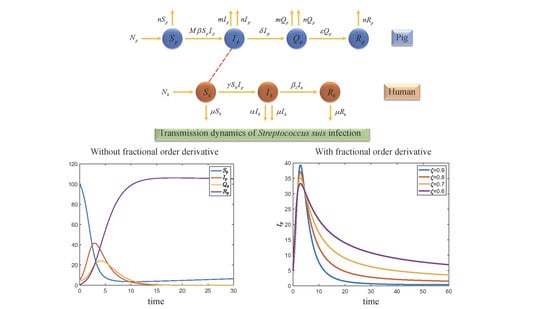
Study of Transmission Dynamics of Streptococcus suis Infection Mathematical Model between Pig and Human under ABC Fractional Order Derivative

Abstract

In this paper, a mathematical model for Streptococcus suis infection is improved by using the fractional order derivative. The modified model also investigates the transmission between pigs and humans. The proposed model can classify the pig population density into four classes, which are pig susceptible class, pig infectious class, pig quarantine class, and pig recovery class. Moreover, the human population density has been separated into three classes, these are human susceptible class, human infectious class, and human recovery class. The spread of the infection is analyzed by considering the contact between humans and pigs. The basic reproduction number $\left(R_0\right)$, the infectious indicator, is carried out using the next generation matrix. The disease-free equilibrium is locally asymptotically stable if $R_0<1$, and the endemic equilibrium is locally asymptotically stable if $R_0>1$. The theoretical analyses of the fractional order derivative model, existence and uniqueness, have been proposed. The numerical examples were illustrated to support the proposed stability theorems. The results show that the fractional order derivative model provides the various possible solution trajectories with different fractional orders for the same parameters. In addition, transmission between pigs and humans resulted in the spread of Streptococcus suis infection.

1. Introduction

One of the biggest problems is the zoonotic pathogen. Recently, the world has faced SARS, influenza, Yellow fever, Avian influenza, MERS, and COVID-19 [1,2,3]. These diseases affect the world’s economy. If we focus only on the swine industry, Streptococcus suis (S. suis) is one of the major problems [4,5,6]. S. suis is a Gram-positive bacterium that is an infectious agent found widely in piglets and pigs around the world [7,8]. It can be found in the respiratory tract, genitals, and alimentary tracts of pigs [9,10]. S. suis transmits rapidly across the farm from pig to pig via direct contact with sick pigs [5,11]. This pathogen has an at least $20\%$ mortality rate in pigs around the world [12]. This disease was first found in 1954 [13,14]. There are at least 35 serotypes of S. suis [15,16]. Moreover, this pathogen can be transmitted to humans via contact with pork [4,17,18]. After that, the number of humans who are infected by this pathogen has increased over the last two decades. Especially, the most commonly found human cases are in Thailand, Vietnam, the Netherlands, and China [9,19,20,21].

Many people die due to the disease. Mathematical models can help to prevent the spread of the disease. They are efficient tools to predict the dynamics of the disease [22,23,24,25]. Fatmawati et al. [26] proposed a new model for dengue fever by using fractional calculus. They also investigated the relationship between mosquitoes and humans. Huang et al. [27] used a price function to express the relation between price and pig stock. Then, they proposed the time delay dynamical model to analyze the dynamics of African swine fever (ASF) disease transmission. Carvalho et al. [28] proposed the mathematical modeling of a dengue epidemic by considering the relation between vectors and humans. Kumar et al. [29] studied the time-delay Caputo fractional order model for plant disease. Peter et al. [30] proposed the fractional order of COVID-19 in Nigeria using the Atangana–Baleanu operator. However, fewer research studies have been conducted on the mathematical models for S. suis infection. Shen et al. [31] introduced the SIQRW model to study the dynamic of S. Suis by using ordinary differential equations. Giang et al. [16] introduced the mathematical model to predict the behavior of the disease, and estimated the parameters in the model with collected data. To our knowledge, no research study has reported on a mathematical model for S. suis using fractional calculus. Fractional calculus is a suitable tool for demonstrating some real-world situations, because it is more generalized than integer-order differential equation systems. In addition, the model can reduce financial losses in the swine industry because the model can forecast disease transmission. Then, the strategies to control the disease are obtained from the model parameters.

In this paper, we improved the mathematical model to predict the disease transmission of S. suis between humans and pigs by using fractional calculus. Firstly, we formulated the model in the form of the system of integer-order differential equations. We also found the basic reproduction number by using the next-generation matrix. The symmetric and asymmetric properties are investigated in the next-generation matrix. Then, we apply the Atagana–Baleanu–Caputo fractional order derivative to the model. The analysis of the proposed model is investigated. We propose the theorem to confirm that the solution of the proposed model exists. We also present numerical examples to confirm the result from the analysis part which are the stability conditions. This means that if the parameters satisfies the stability condition, the solution trajectories will go to the equilibrium. In addition, the basic reproduction number of the model, which is used to describe how fast the disease transmission is, is also studied in this paper.

According to the argument mentioned above, to study endemic S. Suis, a mathematical model is developed by considering the disease transmission between pigs and humans. Basic knowledge about fractional calculus is presented in Section 2. Then, the SIQR-SIR (Susceptible-Infectious-Quarantine-Recovery-Susceptible-Infectious-Recovery) model is introduced in Section 3. The analysis of the mathematical model is shown in Section 4. The fractional order model is presented in Section 5. Then, Section 6 discusses the numerical examples of the proposed model. Finally, conclusions are presented in Section 7.

2. Fractional Calculus

In this section, the related definitions of the fractional operators that are used in this paper are shown as follows.

Definition 1

([32]). The Riemann–Liouville integral operator of the fractional order α for $0<\alpha <1$ for a function $f:(0,\infty )\to \mathbb{R}$ is given by:

$$J_t^{\alpha }f\left(t\right)={\displaystyle \frac{1}{\Gamma \left(\alpha \right)}}{\int }_0^t{(t-s)}^{\alpha -1}f\left(s\right)ds,$$

(1)

where $\Gamma (·)$ is the Gamma function.

Definition 2

([32]). The Caputo fractional derivative for order $\rho >0$ is defined as:

$${}^{\mathcal{C}}{D}_t^{\rho }f\left(t\right)={\displaystyle \frac{1}{\Gamma (n-\rho )}}{\int }_0^t{(t-s)}^{n-\rho -1}{f}^{\left(n\right)}\left(s\right)ds,$$

(2)

where $n-1<\rho \le n,n\in \mathbb{N}$ and $f\in C^{n-1}[0,t].$

Definition 3

([33]). The Atangana–Baleanu fractional derivative for a given function for order ζ in the Caputo sense (ABC) is defined as:

$${}_a^{ABC}{D}_t^{\zeta }f\left(t\right)={\displaystyle \frac{B\left(\zeta \right)}{1-\zeta }}{\int }_a^t{\displaystyle \frac{df\left(s\right)}{ds}}{E}_k\left[{\displaystyle \frac{-\zeta {(1-s)}^{\zeta }}{1-\zeta }}\right]ds,$$

(3)

where $B\left(\zeta \right)=(1-\zeta )+{\displaystyle \frac{\zeta }{\Gamma \left(\zeta \right)}}$ is a normalization function and $E_{\alpha }(·)$ is the Mittag-Leffler function.

Definition 4

([33]). The Atangana–Baleanu fractional integral order ζ is defined as:

$${}_0^{ABC}{I}_t^{\zeta }f\left(t\right)={\displaystyle \frac{1-\zeta }{B\left(\zeta \right)}}f\left(t\right)+{\displaystyle \frac{\zeta }{B\left(\zeta \right)\Gamma \left(\zeta \right)}}{\int }_a^{t}f\left(s\right){(t-s)}^{\zeta -1}ds,$$

(4)

where $B\left(\zeta \right)=(1-\zeta )+{\displaystyle \frac{\zeta }{\Gamma \left(\zeta \right)}}$ is a normalization function.

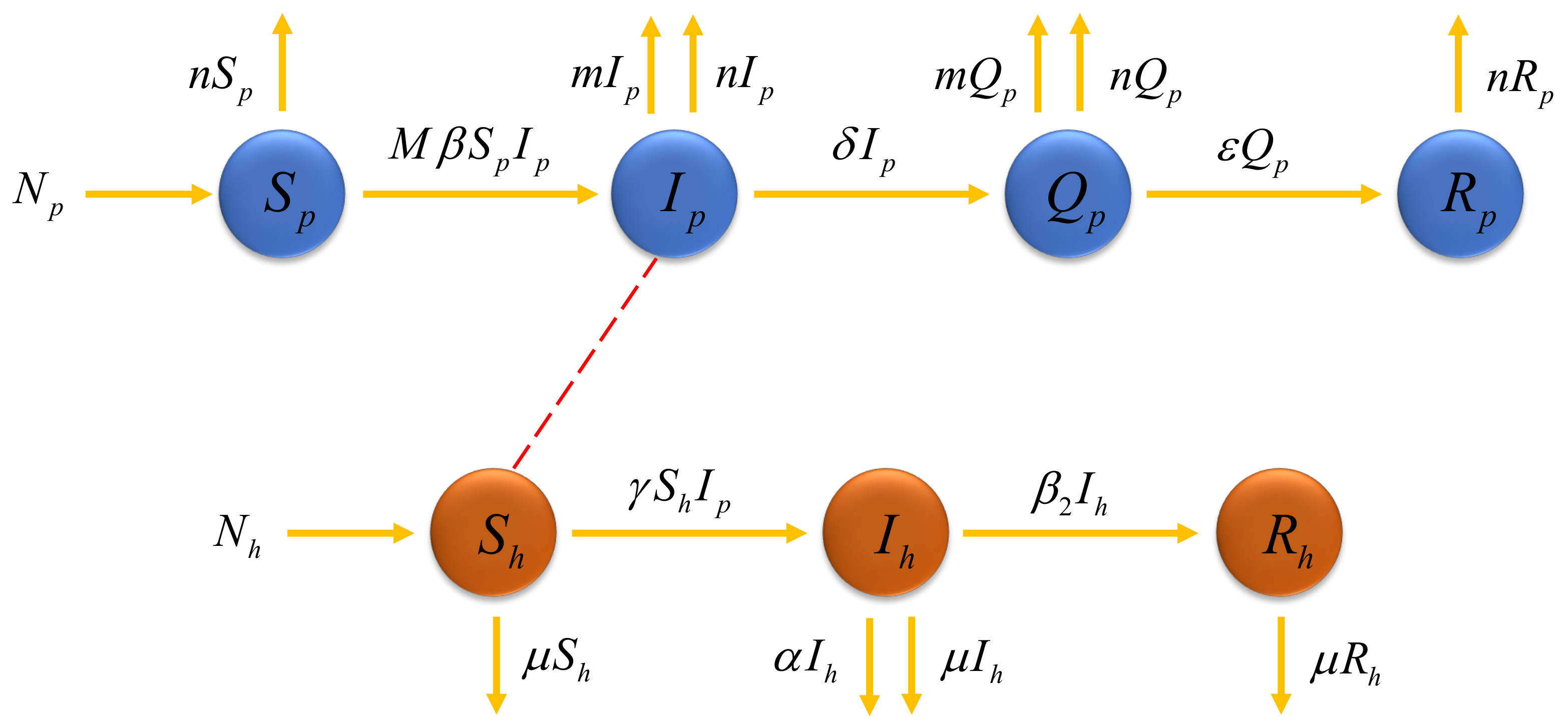
3. Formulation of the Mathematical Model

In this section, we express the model formulation of the disease transmitted in humans and pigs. We classified the pig population into four classes, which are susceptible class ($S_p$), infectious class ($I_p$), quarantine class ($Q_p$), and recovery class ($R_p$). Since the transmission of S. Suis can be transferred between pigs and humans, therefore, the susceptible human class ($S_h$), infectious class ($I_h$), and recovery class ($R_h$) are taken into the model. The flowchart of the SIQR-SIR model of pigs and humans described by the system (5) is shown in Figure 1.

$$\begin{array}{cc}\hfill {\displaystyle \frac{d{S}_p}{dt}}& =N_p-M\beta S_p{I}_p-n{S}_p,\hfill \\ \hfill {\displaystyle \frac{d{I}_p}{dt}}& =M\beta S_p{I}_p-\delta I_p-m{I}_p-n{I}_p,\hfill \\ \hfill {\displaystyle \frac{d{Q}_p}{dt}}& =\delta I_p-m{Q}_p-n{Q}_p-\epsilon Q_p,\hfill \\ \hfill {\displaystyle \frac{d{R}_p}{dt}}& =\epsilon Q_p-n{R}_p,\hfill \\ \hfill {\displaystyle \frac{d{S}_h}{dt}}& =N_h-\mu S_h-\gamma S_h{I}_p,\hfill \\ \hfill {\displaystyle \frac{d{I}_h}{dt}}& =\gamma S_h{I}_p-\alpha I_h-\mu I_h-{\beta }_2{I}_h,\hfill \\ \hfill {\displaystyle \frac{d{R}_h}{dt}}& ={\beta }_2{I}_h-\mu R_h.\hfill \end{array}$$

(5)

The model parameter defined as $\beta$ is the coefficient transmission per unit of time per pig in the pig susceptible class contact with infectious pig class, M is the relative humidity, m is the pig death rate induced by the disease, n is the pig natural death rate, $\delta$ is the rate from infectious class to quarantine class in pigs, $\epsilon$ is the pig recovered rate, $\mu$ is the human natural death rate, $\gamma$ is the transmission rate from infected pig to human, $\alpha$ is the disease death rate, and ${\beta }_2$ is the human recovered rate.

4. Model Analysis

In this section, we investigate the invariant region of the solution of the model, which is biologically meaningful because the proposed model involves the population number. All variables and parameters in the model are assumed to be non-negative. Then, the equilibria of the model and the basic reproduction number are obtained. Moreover, we also study the local stability of all equilibria.

4.1. The Invariant Region

The total population of humans and pigs can be written as

$$N\left(t\right)=S_p+I_p+Q_p+R_p+S_h+I_h+R_h.$$

Differentiating with respect to t of the total population equation, we have

$$\begin{array}{cc}\hfill \frac{dN\left(t\right)}{dt}& =\frac{d{S}_p}{dt}+\frac{d{I}_p}{dt}+\frac{d{Q}_p}{dt}+\frac{d{R}_p}{dt}+\frac{d{S}_h}{dt}+\frac{d{I}_h}{dt}+\frac{d{R}_h}{dt}\hfill \\ \hfill & =N_p+N_h-n(S_p+R_p)-(m+n)(I_p+Q_p)-\mu (S_h+R_h)-(\alpha +\mu )I_p\hfill \\ \hfill & \le N_p+N_h-AN\hfill \end{array}$$

where A is a constant.

Then, we have

$$N\left(t\right)\le \frac{N_p+N_h}{A}+\left(N\left(0\right)-\frac{N_p+N_h}{A}\right)e^{-At}.$$

As $t\to \infty$, the above inequality leads to

$$N\left(t\right)\le \frac{N_p+N_h}{A}.$$

The feasible solution set of population in the system (5) remains in the region

$$\begin{array}{c}\hfill \Omega =\left\{(S_p,I_p,Q_p,R_p,S_h,I_h,R_h)\in {\mathbb{R}}_{+}^7:N\le \frac{N_p+N_h}{A}\right\}.\end{array}$$

4.2. Equilibria

Setting all equations in the system (5) to be zeros, we obtain

$$\begin{array}{cc}\hfill N_p-M\beta S_p{I}_p-n{S}_p& =0,\hfill \\ \hfill M\beta S_p{I}_p-\delta I_p-m{I}_p-n{I}_p& =0,\hfill \\ \hfill \delta I_p-m{Q}_p-n{Q}_p-\epsilon Q_p& =0,\hfill \\ \hfill \epsilon Q_p-n{R}_p& =0,\hfill \\ \hfill N_h-\mu S_h-\gamma S_h{I}_p& =0,\hfill \\ \hfill \gamma S_h{I}_p-\alpha I_h-\mu I_h-{\beta }_2{I}_h& =0,\hfill \\ \hfill {\beta }_2{I}_h-\mu R_h& =0.\hfill \end{array}$$

(6)

The system (5) has two types of equilibrium points, which are disease-free equilibrium (DFE), the point at which no disease is, and endemic equilibrium, where the infection is constantly maintained at some level [34,35].

The disease-free equilibrium (DFE) of the system (5) can be written as

$$E_1=\left({\displaystyle \frac{N_p}{n},0,0,0,\frac{N_h}{\mu },0,0}\right).$$

The endemic equilibrium of the system (5) is

$$E_2=\left({\displaystyle \frac{\delta +m+n}{M\beta },\frac{n(R_0-1)}{M\beta },\frac{\delta I_p}{m+n+\epsilon },\frac{\epsilon Q_p}{n},\frac{N_{h}M\beta }{\mu M\beta +n\gamma (R_0-1)},\frac{\gamma S_h{I}_p}{\alpha +\mu +{\beta }_2},\frac{{\beta }_2{I}_h}{\mu }}\right).$$

4.3. Basic Reproduction Number $\left(R_0\right)$

The next generation matrix method [36] is used to compute the basic reproduction number $\left(R_0\right)$. In addition, the local stability of the equilibrium of the system (5) can be considered by using the basic reproduction number. By following the process as [37], we have

$$f=\left[\begin{array}{c}M\beta S_p{I}_p\\ \delta I_p\\ \gamma S_h{I}_p\end{array}\right],v=\left[\begin{array}{c}\delta I_p+m{I}_p+n{I}_p\\ m{Q}_p+n{Q}_p+\epsilon Q_p\\ \alpha I_h+\mu I_h+{\beta }_2{I}_h\end{array}\right].$$

The corresponding asymmetry Jacobian matrix of f and v are

$$F=\left[\begin{array}{ccc}M\beta S_p& 0& 0\\ \delta & 0& 0\\ \gamma S_h& 0& 0\end{array}\right],V=\left[\begin{array}{ccc}\delta +m+n& 0& 0\\ 0& m+n+\epsilon & 0\\ \alpha & 0& \mu +{\beta }_2\end{array}\right].$$

Then, we have

$$V^{-1}=\left[\begin{array}{ccc}\frac{1}{\delta +m+n}& 0& 0\\ 0& \frac{1}{m+n+\epsilon }& 0\\ \frac{-\alpha }{(\delta +m+n)(\mu +{\beta }_2)}& 0& \frac{1}{\mu +{\beta }_2}\end{array}\right].$$

Therefore,

$$F{V}^{-1}=\left[\begin{array}{ccc}\frac{M\beta S_p}{\delta +m+n}& 0& 0\\ \frac{\delta }{\delta +m+n}& 0& 0\\ \frac{\gamma S_h}{\delta +m+n}& 0& 0\end{array}\right].$$

The eigenvalues of $F{V}^{-1}$ are

$${\lambda }_1=0,{\lambda }_2=0,{\lambda }_3=\frac{M\beta S_p}{\delta +m+n}.$$

We thus have the basic reproduction number, which is the spectral radius

$${\displaystyle R_0=\frac{M\beta S_p}{\delta +m+n}.}$$

4.4. The Stability of Disease-Free Equilibrium

In this subsection, the disease-free equilibrium $E_1$ is shown, where $E_1$ is locally asymptotically stable when $R_0<1$. The method is to investigate the eigenvalues of the Jacobian matrix of the linearized system of the model (5) at the equilibrium.

Theorem 1.

The disease-free equilibrium point $\left(E_1\right)$ is locally asymptotically stable if $R_0<1$.

Proof. 

The Jacobian matrix at the disease-free equilibrium $\left(E_1\right)$ of the system (5) is

$$J\left(E_1\right)=\left[\begin{array}{ccccccc}-n& -M\beta \frac{N_p}{n}& 0& 0& 0& 0& 0\\ 0& M\beta \frac{N_p}{n}-\delta -\omega & 0& 0& 0& 0& 0\\ 0& \delta & -\omega -\epsilon & 0& 0& 0& 0\\ 0& 0& \epsilon & -n& 0& 0& 0\\ 0& -\gamma \frac{N_h}{\mu }& 0& 0& -\mu & 0& 0\\ 0& \gamma \frac{N_h}{\mu }& 0& 0& 0& -\alpha -\mu -{\beta }_2& 0\\ 0& 0& 0& 0& 0& {\beta }_2& -\mu \end{array}\right].$$

The eigenvalues of the Jacobian matrix $J\left(E_1\right)$ are

$$\begin{array}{cc}\hfill {\lambda }_1& =-\alpha -\mu -{\beta }_2,\hfill \\ \hfill {\lambda }_2& =-\omega -\epsilon ,\hfill \\ \hfill {\lambda }_3& ={\lambda }_4=-\mu ,\hfill \\ \hfill {\lambda }_5& ={\lambda }_6=-n,\hfill \\ \hfill {\lambda }_7& {\displaystyle =\frac{M\beta N_p-n(\delta -\omega )}{n}=(\delta +\omega )(R_0-1).}\hfill \end{array}$$

We have that ${\lambda }_7<0$ when $R_0<1$. Therefore, the disease-free equilibrium $\left(E_1\right)$ of the system (5) is locally asymptotically stable when $R_1<1$. □

4.5. The Stability of Endemic Equilibrium

In this subsection, the endemic equilibrium $E_2$ is shown, where $E_2$ is locally asymptotically stable when $R_0>1$. The method is to investigate the eigenvalues of the Jacobian matrix $J\left(E_2\right)$ of the linearized system of the model (5) at the equilibrium. The Jacobian matrix method has been used in [38].

Theorem 2.

The endemic equilibrium $\left(E_2\right)$ is locally asymptotically stable if $R_0>1$.

Proof. 

The endemic equilibrium

$$E_2=\left(\frac{\delta +\omega }{M\beta },\frac{n(R_0-1)}{M\beta },\frac{\delta I_p}{\omega +\epsilon },\frac{\epsilon Q_p}{n},\frac{N_{h}M\beta }{\mu M\beta +n\gamma (R_0-1)},\frac{\gamma S_h{I}_p}{\alpha +\mu +{\beta }_2},\frac{{\beta }_2{I}_h}{\mu }\right)$$

is positive and epidemiologically meaningful if $R_0>1$.

The Jacobian matrix at the endemic equilibrium $\left(E_2\right)$ of the system (5) is

$$J\left(E_2\right)=\left[\begin{array}{ccccccc}-n(R_0-1)-n& -\delta -\omega & 0& 0& 0& 0& 0\\ n(R_0-1)& 0& 0& 0& 0& 0& 0\\ 0& \delta & -\omega -\epsilon & 0& 0& 0& 0\\ 0& 0& \epsilon & -n& 0& 0& 0\\ 0& -B& 0& 0& -\mu -\gamma C& 0& 0\\ 0& B& 0& 0& \gamma C& -\alpha -\mu -{\beta }_2& 0\\ 0& 0& 0& 0& 0& {\beta }_2& -\mu \end{array}\right]$$

where

$$B=\frac{\gamma N_h}{{\displaystyle \frac{n(R_0-1)\gamma }{M\beta }+\mu }},C=\frac{n(R_0-1)}{M\beta }.$$

The eigenvalues of the Jacobian matrix $J\left(E_2\right)$ are

$$\begin{array}{cc}\hfill {\lambda }_1& =-n,\hfill \\ \hfill {\lambda }_2& =-\mu ,\hfill \\ \hfill {\lambda }_3& =-\omega -\epsilon ,\hfill \\ \hfill {\lambda }_4& =-\alpha -\mu {\beta }_2,\hfill \\ \hfill {\lambda }_5& =-\frac{M\beta \mu +n\gamma (R_0-1)}{M\beta },\hfill \\ \hfill {\lambda }_6& =-\frac{1}{2}n{R}_0+\frac{1}{2}\sqrt{n^2{R}_0^2-4\delta n{R}_0-4mn{R}_0-4n^2{R}_0+4\delta n+4mn+4n^2}\hfill \\ \hfill & =-\frac{1}{2}n{R}_0+\frac{1}{2}\sqrt{n^2{R}_0^2-4(\delta n+mn+n^2)(R_0-1)},\hfill \\ \hfill {\lambda }_7& =-\frac{1}{2}n{R}_0-\frac{1}{2}\sqrt{n^2{R}_0^2-4\delta n{R}_0-4mn{R}_0-4n^2{R}_0+4\delta n+4mn+4n^2}\hfill \\ \hfill & =-\frac{1}{2}n{R}_0-\frac{1}{2}\sqrt{n^2{R}_0^2-4(\delta n+mn+n^2)(R_0-1)}.\hfill \end{array}$$

We have that ${\lambda }_5<0$ when $R_0>1$.

We next consider ${\lambda }_6$ and ${\lambda }_7$ are negative if $(\delta n+mn+n^2)(R_0-1)<0$. This means that $R_0>1$.

Therefore, the endemic equilibrium $\left(E_2\right)$ of the system (5) is locally asymptotically stable when $R_0>1$. □

5. The Fractional Order Model with the Atangana–Baleanu–Caputo Operator

The improved model by using Atangana–Baleanu–Caputo (ABC) fractional derivative to the proposed model (5) given by a system of ordinary differential equation can be written as the following system.

$$\begin{array}{cc}\hfill {\displaystyle {}_0^{ABC}{D}^{\zeta }{S}_p\left(t\right)}& ={\Psi }_1(t,S_p\left(t\right))=N_p-M\beta S_p{I}_p-n{S}_p\hfill \\ \hfill {\displaystyle {}_0^{ABC}{D}^{\zeta }{I}_p\left(t\right)}& ={\Psi }_2(t,I\left(t\right))=M\beta S_p{I}_p-\delta I_p-m{I}_p-n{I}_p\hfill \\ \hfill {\displaystyle {}_0^{ABC}{D}^{\zeta }{Q}_p\left(t\right)}& ={\Psi }_3(t,Q\left(t\right))=\delta I_p-m{Q}_p-n{Q}_p-\epsilon Q_p\hfill \\ \hfill {\displaystyle {}_0^{ABC}{D}^{\zeta }{R}_p\left(t\right)}& ={\Psi }_4(t,R_p\left(t\right))=\epsilon Q_p-n{R}_p\hfill \\ \hfill {\displaystyle {}_0^{ABC}{D}^{\zeta }{S}_h\left(t\right)}& ={\Psi }_5(t,S_h\left(t\right))=N_h-\mu S_h-\gamma S_h{I}_p\hfill \\ \hfill {\displaystyle {}_0^{ABC}{D}^{\zeta }{I}_h\left(t\right)}& ={\Psi }_6(t,I_h\left(t\right))=\gamma S_h{I}_p-\alpha I_h-\mu I_h\hfill \\ \hfill {\displaystyle {}_0^{ABC}{D}^{\zeta }{R}_h\left(t\right)}& ={\Psi }_7(t,R_h\left(t\right))={\beta }_2{I}_h-\mu R_h-{\beta }_2{I}_h\hfill \end{array}$$

(7)

The notation ${}_0^{ABC}{D}^{\zeta }$ is the time fractional derivative in Atangana–Baleanu with Caputo sense and the parameter $0<\zeta \le 1$ is the order of the ABC operator with the initial conditions

$$\begin{array}{cc}\hfill & S_{p_0}\left(t\right)=S_p\left(0\right),I_{p_0}\left(t\right)=I_p\left(0\right),Q_{p_0}\left(t\right)=Q_p\left(0\right),R_{p_0}\left(t\right)=R_p\left(0\right),\hfill \\ \hfill & S_{h_0}\left(t\right)=S_h\left(0\right),I_{h_0}\left(t\right)=I_h\left(0\right),R_{h_0}\left(t\right)=R_h\left(0\right).\hfill \end{array}$$

(8)

The system (7) can be written as the Voltera integral equation by using the ABC integral operator as follows:

$$\begin{array}{cc}\hfill {\displaystyle S_{p_0}\left(t\right)-S_p\left(0\right)=}& \frac{1-\zeta }{B\left(\zeta \right)}(N_p-M\beta S_p\left(t\right)I_p\left(t\right)-n{S}_p\left(t\right))\hfill \\ \hfill {\displaystyle }& +\frac{\zeta }{B\left(\zeta \right)\Gamma \left(\zeta \right)}{\int }_0^t(N_p-M\beta S_p\left(z\right)I_p\left(s\right)-n{S}_p\left(z\right)){(t-z)}^{\zeta -1}dz\hfill \\ \hfill {\displaystyle I_{p_0}\left(t\right)-I_p\left(0\right)=}& \frac{1-\zeta }{B\left(\zeta \right)}(M\beta S_p\left(t\right)I_p\left(t\right)-(\delta +m+n)I_p(\Psi ))\hfill \\ \hfill {\displaystyle }& +\frac{\zeta }{B\left(\zeta \right)\Gamma \left(\zeta \right)}{\int }_0^t(M\beta S_p\left(z\right)I_p\left(z\right)-(\delta +m+n)I_p\left(z\right)){(t-z)}^{\zeta -1}dz\hfill \\ \hfill {\displaystyle Q_{p_0}\left(t\right)-Q_p\left(0\right)=}& \frac{1-\zeta }{B\left(\zeta \right)}(\delta I_p\left(t\right)-(m+n+\epsilon )Q_p\left(t\right))\hfill \\ \hfill {\displaystyle }& +\frac{\zeta }{B\left(\zeta \right)\Gamma \left(\zeta \right)}{\int }_0^t(\delta I_p\left(z\right)-(m+n+\epsilon )Q_p\left(z\right)){(t-z)}^{\zeta -1}dz\hfill \\ \hfill {\displaystyle R_{p_0}\left(t\right)-R_p\left(0\right)=}& \frac{1-\zeta }{B\left(\zeta \right)}(\epsilon Q_p\left(t\right)-n{R}_p\left(t\right))\hfill \\ \hfill {\displaystyle }& +\frac{k}{B\left(K\right)\Gamma \left(\zeta \right)}{\int }_0^t(\epsilon Q_p\left(z\right)-n{R}_p\left(z\right)){(t-z)}^{\zeta -1}dz\hfill \\ \hfill {\displaystyle S_{h_0}\left(t\right)-S_h\left(0\right)=}& \frac{1-\zeta }{B\left(\zeta \right)}(N_h-\mu S_h\left(t\right)-\gamma S_h\left(t\right)I_p\left(t\right))\hfill \\ \hfill {\displaystyle }& +\frac{\zeta }{B\left(\zeta \right)\Gamma \left(\zeta \right)}{\int }_0^t(N_h-\mu S_h\left(z\right)-\gamma S_h\left(z\right)I_p\left(z\right)){(t-z)}^{\zeta -1}dz\hfill \\ \hfill {\displaystyle I_{h_0}\left(t\right)-I_h\left(0\right)=}& \frac{1-\zeta }{B\left(\zeta \right)}(\gamma S_h{I}_p-(\alpha +\mu +\beta -2)I_h\left(t\right))\hfill \\ \hfill {\displaystyle }& +\frac{\zeta }{B\left(\zeta \right)\Gamma \left(\zeta \right)}{\int }_0^t(\gamma S_h{I}_p-(\alpha +\mu +\beta -2)I_h\left(z\right)){(t-z)}^{\zeta -1}dz\hfill \\ \hfill {\displaystyle R_{h_0}\left(t\right)-R_h\left(0\right)=}& \frac{1-\zeta }{B\left(\zeta \right)}({\beta }_2{I}_h-\mu R_h)\hfill \\ \hfill {\displaystyle }& +\frac{\zeta }{B\left(\zeta \right)\Gamma \left(\zeta \right)}{\int }_0^t({\beta }_2{I}_h-\mu R_h){(t-z)}^{\zeta -1}dz.\hfill \end{array}$$

(9)

To confirm the existence of the solution of modification model [39,40], we propose the following theorems.

Theorem 3.

The kernels ${\Psi }_1,{\Psi }_2,{\Psi }_3,{\Psi }_4,{\Psi }_5,{\Psi }_6,{\Psi }_7$ given by the system (7) satisfy the Lipschitz condition and contraction if the following inequalities hold: $0\le {\xi }_i<1$ for all $i=1,2,\dots ,7.$

Proof. 

Let the kernel ${\Psi }_1(t,S\left(t\right))=N_p-M\beta S_p{I}_p-n{S}_p.$

Let $S_{p_1}$ and $S_{p_2}$ be two functions, then we obtain the following

$$\begin{array}{cc}\hfill \parallel {\Psi }_1(t,S_{p_1}\left(t\right))-{\Psi }_1(t,S_{p_2}\left(t\right))\parallel =& \parallel (N_p-M\beta S_{p1}\left(t\right)I_p\left(t\right)-n{S}_{p1}\left(t\right))\hfill \\ \hfill & -(N_p-M\beta S_{p2}\left(t\right)I_p\left(t\right)-n{S}_{p2}\left(t\right))\parallel \hfill \\ \hfill =& \parallel -M\beta I_p\left(t\right)(S_{p1}-S_{p2})\left(t\right)-n(S_{p1}\left(t\right)-S_{p2}\left(t\right))\parallel \hfill \\ \hfill \le & (M\beta \parallel I_p\left(t\right)\parallel +n)\parallel S_{p1}\left(t\right)-S_{p2}\left(t\right)\parallel \hfill \\ \hfill \le & (M\beta L_1+n)\parallel S_{p1}\left(t\right)-S_{p2}\left(t\right)\parallel \hfill \\ \hfill \le & {\xi }_1\parallel S_{p1}\left(t\right)-S_{p2}\left(t\right)\parallel ,\hfill \end{array}$$

where ${\xi }_1=M\beta L_1+n$ and $L_1={max}_{t\in J}\parallel I_p\left(t\right)\parallel$.

In the same manner, we obtain

$$\begin{array}{cc}\hfill \parallel {\Psi }_2(t,S_{p1}\left(t\right))-{\Psi }_2(t,S_{p2}\left(t\right))\parallel & \le {\xi }_2\parallel I_{p1}\left(t\right)-I_{p2}\left(t\right)\parallel ,\hfill \\ \hfill \parallel {\Psi }_3(t,S_{p1}\left(t\right))-{\Psi }_3(t,S_{p2}\left(t\right))\parallel & \le {\xi }_3\parallel Q_{p1}\left(t\right)-Q_{p2}\left(t\right)\parallel ,\hfill \\ \hfill \parallel {\Psi }_4(t,S_{p1}\left(t\right))-{\Psi }_4(t,S_{p2}\left(t\right))\parallel & \le {\xi }_4\parallel R_{p1}\left(t\right)-R_{p2}\left(t\right)\parallel ,\hfill \\ \hfill \parallel {\Psi }_5(t,S_{p1}\left(t\right))-{\Psi }_5(t,S_{p2}\left(t\right))\parallel & \le {\xi }_5\parallel S_{h1}\left(t\right)-S_{h2}\left(t\right)\parallel ,\hfill \\ \hfill \parallel {\Psi }_6(t,S_{p1}\left(t\right))-{\Psi }_6(t,S_{p2}\left(t\right))\parallel & \le {\xi }_6\parallel I_{h1}\left(t\right)-I_{h2}\left(t\right)\parallel ,\hfill \\ \hfill \parallel {\Psi }_7(t,S_{p1}\left(t\right))-{\Psi }_7(t,S_{p2}\left(t\right))\parallel & \le {\xi }_7\parallel R_{h1}\left(t\right)-R_{h2}\left(t\right)\parallel ,\hfill \end{array}$$

(10)

where

$$\begin{array}{cc}\hfill {\xi }_2& =M\beta L_2-(\delta +m+n),\hfill \\ \hfill {\xi }_3& =m+n+\delta ,\hfill \\ \hfill {\xi }_4& =n,\hfill \\ \hfill {\xi }_5& =\mu +\gamma L_3,\hfill \\ \hfill {\xi }_6& =\alpha +\mu +{\beta }_2,\hfill \\ \hfill {\xi }_7& =\mu ,\hfill \end{array}$$

with $L_2={max}_{t\in J}\parallel S_p\left(t\right)\parallel ,L_3={max}_{t\in J}\parallel I_p\left(t\right)\parallel .$

Considering the kernels of the model, we can write the Equation (9) as

$$\begin{array}{cc}\hfill S_p\left(t\right)& =S_p\left(0\right)+\frac{1-\zeta }{B\left(\zeta \right)}\left({\Psi }_1(t,S_p\left(t\right))\right)+\frac{\zeta }{B\left(\zeta \right)\Gamma \left(\zeta \right)}{\int }_0^t\left({\Psi }_1(z,S_p\left(z\right))\right){(t-z)}^{\zeta -1}dz,\hfill \\ \hfill I_p\left(t\right)& =I_p\left(0\right)+\frac{1-\zeta }{B\left(\zeta \right)}\left({\Psi }_2(t,I_p\left(t\right))\right)+\frac{\zeta }{B\left(\zeta \right)\Gamma \left(\zeta \right)}{\int }_0^t\left({\Psi }_2(z,I_p\left(z\right))\right){(t-z)}^{\zeta -1}dz,\hfill \\ \hfill Q_p\left(t\right)& =Q_p\left(0\right)+\frac{1-\zeta }{B\left(\zeta \right)}\left({\Psi }_3(t,Q_p\left(t\right))\right)+\frac{\zeta }{B\left(\zeta \right)\Gamma \left(\zeta \right)}{\int }_0^t\left({\Psi }_3(z,Q_p\left(z\right))\right){(t-z)}^{\zeta -1}dz,\hfill \\ \hfill R_p\left(t\right)& =R_p\left(0\right)+\frac{1-\zeta }{B\left(\zeta \right)}\left({\Psi }_4(t,R_p\left(t\right))\right)+\frac{\zeta }{B\left(\zeta \right)\Gamma \left(\zeta \right)}{\int }_0^t\left({\Psi }_4(z,R_p\left(z\right))\right){(t-z)}^{\zeta -1}dz,\hfill \\ \hfill S_h\left(t\right)& =S_h\left(0\right)+\frac{1-\zeta }{B\left(\zeta \right)}\left({\Psi }_5(t,S_h\left(t\right))\right)+\frac{\zeta }{B\left(\zeta \right)\Gamma \left(\zeta \right)}{\int }_0^t\left({\Psi }_5(z,S_h\left(z\right))\right){(t-z)}^{\zeta -1}dz,\hfill \\ \hfill I_h\left(t\right)& =I_h\left(0\right)+\frac{1-\zeta }{B\left(\zeta \right)}\left({\Psi }_6(t,I_h\left(t\right))\right)+\frac{\zeta }{B\left(\zeta \right)\Gamma \left(\zeta \right)}{\int }_0^t\left({\Psi }_6(z,I_h\left(z\right))\right){(t-z)}^{\zeta -1}dz,\hfill \\ \hfill R_h\left(t\right)& =R_h\left(0\right)+\frac{1-\zeta }{B\left(\zeta \right)}\left({\Psi }_7(t,R_h\left(t\right))\right)+\frac{\zeta }{B\left(\zeta \right)\Gamma \left(\zeta \right)}{\int }_0^t\left({\Psi }_7(z,R_h\left(z\right))\right){(t-z)}^{\zeta -1}dz.\hfill \end{array}$$

(11)

Therefore, we obtain the following recursive formula.

$$\begin{array}{cc}\hfill S_{p_n}\left(t\right)=& S_p\left(0\right)+\frac{1-\zeta }{B\left(\zeta \right)}\left({\Psi }_1(t,S_{p_{n-1}}\left(t\right))\right)+\frac{\zeta }{B\left(\zeta \right)\Gamma \left(\zeta \right)}{\int }_0^t\left({\Psi }_1(z,S_{p_{n-1}}\left(z\right))\right){(t-z)}^{\zeta -1}dz,\hfill \\ \hfill I_{p_n}\left(t\right)=& I_p\left(0\right)+\frac{1-\zeta }{B\left(\zeta \right)}\left({\Psi }_2(t,I_{p_{n-1}}\left(t\right))\right)+\frac{\zeta }{B\left(\zeta \right)\Gamma \left(\zeta \right)}{\int }_0^t\left({\Psi }_2(z,I_{p_{n-1}}\left(z\right))\right){(t-z)}^{\zeta -1}dz,\hfill \\ \hfill Q_{p_n}\left(t\right)=& Q_p\left(0\right)+\frac{1-\zeta }{B\left(\zeta \right)}\left({\Psi }_3(t,Q_{p_{n-1}}\left(t\right))\right)+\frac{\zeta }{B\left(\zeta \right)\Gamma \left(\zeta \right)}{\int }_0^t\left({\Psi }_3(z,Q_{p_{n-1}}\left(z\right))\right){(t-z)}^{\zeta -1}dz,\hfill \\ \hfill R_{p_n}\left(t\right)=& R_p\left(0\right)+\frac{1-\zeta }{B\left(\zeta \right)}\left({\Psi }_4(t,R_{p_{n-1}}\left(t\right))\right)+\frac{\zeta }{B\left(\zeta \right)\Gamma \left(\zeta \right)}{\int }_0^t\left({\Psi }_4(z,R_{p_{n-1}}\left(z\right))\right){(t-z)}^{\zeta -1}dz,\hfill \\ \hfill S_{h_n}\left(t\right)=& S_h\left(0\right)+\frac{1-\zeta }{B\left(\zeta \right)}\left({\Psi }_5(t,S_{h_{n-1}}\left(t\right))\right)+\frac{\zeta }{B\left(\zeta \right)\Gamma \left(\zeta \right)}{\int }_0^t\left({\Psi }_5\left(z{S}_{h_{n-1}}\left(z\right)\right)\right){(t-z)}^{\zeta -1}dz,\hfill \\ \hfill I_{h_n}\left(t\right)=& I_h\left(0\right)+\frac{1-\zeta }{B\left(\zeta \right)}\left({\Psi }_6(t,I_{h_{n-1}}\left(t\right))\right)+\frac{\zeta }{B\left(\zeta \right)\Gamma \left(\zeta \right)}{\int }_0^t\left({\Psi }_6(z,I_{h_{n-1}}\left(z\right))\right){(t-z)}^{\zeta -1}dz,\hfill \\ \hfill R_{h_n}\left(t\right)=& R_h\left(0\right)+\frac{1-\zeta }{B\left(\zeta \right)}\left({\Psi }_7(t,R_{h_{n-1}}\left(t\right))\right)+\frac{\zeta }{B\left(\zeta \right)\Gamma \left(\zeta \right)}{\int }_0^t\left({\Psi }_7(z,R_{h_{n-1}}\left(z\right))\right){(t-z)}^{\zeta -1}dz.\hfill \end{array}$$

(12)

We then obtain the difference between the iterative terms in the expression

$$\begin{array}{cc}\hfill {{\rm Y}}_{1_n}=& S_{p_n}\left(t\right)-S_{p_{n-1}}\left(t\right)=\frac{1-\zeta }{B\left(\zeta \right)}({\Psi }_1(t,S_{p_{n-1}}\left(t\right))-{\Psi }_1(t,S_{p_{n-2}}\left(t\right)))\hfill \\ \hfill & +\frac{\zeta }{B\left(\zeta \right)\Gamma \left(\zeta \right)}{\int }_0^t({\Psi }_1(\xi ,S_{p_{n-1}}\left(t\right))-{\Psi }_1(\xi ,S_{p_{n-2}}\left(\xi \right))){(t-\xi )}^{\zeta -1}d\xi ,\hfill \\ \hfill {{\rm Y}}_{2_n}=& I_{p_n}\left(t\right)-I_{p_{n-1}}\left(t\right)=\frac{1-\zeta }{B\left(\zeta \right)}({\Psi }_2(t,I_{p_{n-1}}\left(t\right))-{\Psi }_2(t,I_{p_{n-2}}\left(t\right)))\hfill \\ \hfill & +\frac{\zeta }{B\left(\zeta \right)\Gamma \left(\zeta \right)}{\int }_0^t({\Psi }_2(\xi ,S_{p_{n-1}}\left(t\right))-{\Psi }_2(\xi ,I_{p_{n-2}}\left(\xi \right))){(t-\xi )}^{\zeta -1}d\xi ,\hfill \\ \hfill {{\rm Y}}_{3_n}=& Q_{p_n}\left(t\right)-Q_{p_{n-1}}\left(t\right)=\frac{1-\zeta }{B\left(\zeta \right)}({\Psi }_3(t,Q_{p_{n-1}}\left(t\right))-{\Psi }_3(t,Q_{p_{n-2}}\left(t\right)))\hfill \\ \hfill & +\frac{\zeta }{B\left(\zeta \right)\Gamma \left(\zeta \right)}{\int }_0^t({\Psi }_3(\xi ,Q_{p_{n-1}}\left(t\right))-{\Psi }_3(\xi ,Q_{p_{n-2}}\left(\xi \right))){(t-\xi )}^{\zeta -1}d\xi ,\hfill \\ \hfill {{\rm Y}}_{4_n}=& R_{p_n}\left(t\right)-R_{p_{n-1}}\left(t\right)=\frac{1-\zeta }{B\left(\zeta \right)}({\Psi }_4(t,R_{p_{n-1}}\left(t\right))-{\Psi }_4(t,R_{p_{n-2}}\left(t\right)))\hfill \\ \hfill & +\frac{\zeta }{B\left(\zeta \right)\Gamma \left(\zeta \right)}{\int }_0^t({\Psi }_4(\xi ,R_{p_{n-1}}\left(t\right))-{\Psi }_4(\xi ,R_{p_{n-2}}\left(\xi \right))){(t-\xi )}^{\zeta -1}d\xi ,\hfill \\ \hfill {{\rm Y}}_{5_n}=& S_{h_n}\left(t\right)-S_{h_{n-1}}\left(t\right)=\frac{1-\zeta }{B\left(\zeta \right)}({\Psi }_5(t,S_{h_{n-1}}\left(t\right))-{\Psi }_5(t,S_{h_{n-2}}\left(t\right)))\hfill \\ \hfill & +\frac{\zeta }{B\left(\zeta \right)\Gamma \left(\zeta \right)}{\int }_0^t({\Psi }_5(\xi ,S_{h_{n-1}}\left(t\right))-{\Psi }_5(\xi ,S_{h_{n-2}}\left(\xi \right))){(t-\xi )}^{\zeta -1}d\xi ,\hfill \\ \hfill {{\rm Y}}_{6_n}=& I_{h_n}\left(t\right)-I_{h_{n-1}}\left(t\right)=\frac{1-\zeta }{B\left(\zeta \right)}({\Psi }_6(t,I_{h_{n-1}}\left(t\right))-{\Psi }_6(t,I_{h_{n-2}}\left(t\right)))\hfill \\ \hfill & +\frac{\zeta }{B\left(\zeta \right)\Gamma \left(\zeta \right)}{\int }_0^t({\Psi }_6(\xi ,I_{h_{n-1}}\left(t\right))-{\Psi }_6(\xi ,I_{h_{n-2}}\left(\xi \right))){(t-\xi )}^{\zeta -1}d\xi ,\hfill \\ \hfill {{\rm Y}}_{7_n}=& R_{h_n}\left(t\right)-R_{h_{n-1}}\left(t\right)=\frac{1-\zeta }{B\left(\zeta \right)}({\Psi }_7(t,R_{h_{n-1}}\left(t\right))-{\Psi }_7(t,R_{h_{n-2}}\left(t\right)))\hfill \\ \hfill & +\frac{\zeta }{B\left(\zeta \right)\Gamma \left(\zeta \right)}{\int }_0^t({\Psi }_7(\xi ,R_{h_{n-1}}\left(t\right))-{\Psi }_7(\xi ,R_{h_{n-2}}\left(\xi \right))){(t-\xi )}^{\zeta -1}d\xi ,\hfill \end{array}$$

(13)

where

$$S_{p_n}=\sum _{m=1}^n{{\rm Y}}_{1_m},I_{p_n}=\sum _{m=1}^n{{\rm Y}}_{2_m},Q_{p_n}=\sum _{m=1}^n{{\rm Y}}_{3_m},R_{p_n}=\sum _{m=1}^n{{\rm Y}}_{4_m},$$

$$S_{h_n}=\sum _{m=1}^n{{\rm Y}}_{5_m},I_{hn}=\sum _{m=1}^n{{\rm Y}}_{6_m},R_{h_n}=\sum _{m=1}^n{{\rm Y}}_{7_m}.$$

Applying the norm of both sides and considering the triangular inequality, Equation (13) becomes

$$\begin{array}{cc}\hfill \parallel {{\rm Y}}_{1_n}\left(t\right)\parallel =& \parallel S_{p_n}\left(t\right)-S_{pn-1}\left(t\right)\parallel \hfill \\ \hfill \le & \frac{1-\zeta }{B\left(\zeta \right)}\parallel {\Psi }_1(t,S_{pn-1}\left(t\right))-{\Psi }_1(t,S_{pn-2}\left(t\right))\parallel \hfill \\ \hfill & +\frac{\zeta }{B\left(\zeta \right)\Gamma \left(\zeta \right)}\parallel {\int }_0^t\{{\Psi }_1(\Psi ,S_{pn-1}(\Psi ))-{\Psi }_1(\Psi ,S_{pn-2}(\Psi ))\}{(t-\Psi )}^{\zeta -1}\parallel ,\hfill \\ \hfill \parallel {{\rm Y}}_{2_n}\left(t\right)\parallel =& \parallel I_{p_n}\left(t\right)-I_{pn-1}\left(t\right)\parallel \hfill \\ \hfill \le & \frac{1-\zeta }{B\left(\zeta \right)}\parallel {\Psi }_2(t,I_{pn-1}\left(t\right))-{\Psi }_2(t,I_{pn-2}\left(t\right))\parallel \hfill \\ \hfill & +\frac{\zeta }{B\left(\zeta \right)\Gamma \left(\zeta \right)}\parallel {\int }_0^t\{{\Psi }_2(\xi ,I_{pn-1}\left(\xi \right))-{\Psi }_2(\xi ,I_{pn-2}\left(\xi \right))\}{(t-\xi )}^{\zeta -1}\parallel ,\hfill \\ \hfill \parallel {{\rm Y}}_{3_n}\left(t\right)\parallel =& \parallel Q_{p_n}\left(t\right)-Q_{pn-1}\left(t\right)\parallel \hfill \\ \hfill \le & \frac{1-\zeta }{B\left(\zeta \right)}\parallel {\Psi }_3(t,Q_{pn-1}\left(t\right))-{\Psi }_3(t,Q_{pn-2}\left(t\right))\parallel \hfill \\ \hfill & +\frac{\zeta }{B\left(\zeta \right)\Gamma \left(\zeta \right)}\parallel {\int }_0^t\{{\Psi }_3(\xi ,Q_{pn-1}\left(\xi \right))-{\Psi }_3(\xi ,Q_{pn-2}\left(\xi \right))\}{(t-\xi )}^{\zeta -1}\parallel ,\hfill \\ \hfill \parallel {{\rm Y}}_{4_n}\left(t\right)\parallel =& \parallel R_{p_n}\left(t\right)-R_{pn-1}\left(t\right)\parallel \hfill \\ \hfill \le & \frac{1-\zeta }{B\left(\zeta \right)}\parallel {\Psi }_4(t,R_{pn-1}\left(t\right))-{\Psi }_4(t,R_{pn-2}\left(t\right))\parallel \hfill \\ \hfill & +\frac{\zeta }{B\left(\zeta \right)\Gamma \left(\zeta \right)}\parallel {\int }_0^t\{{\Psi }_4(\xi ,R_{pn-1}\left(\xi \right))-{\Psi }_4(\xi ,R_{pn-2}\left(\xi \right))\}{(t-\xi )}^{\zeta -1}\parallel ,\hfill \\ \hfill \parallel {{\rm Y}}_{5_n}\left(t\right)\parallel =& \parallel S_{h_n}\left(t\right)-S_{hn-1}\left(t\right)\parallel \hfill \\ \hfill \le & \frac{1-\zeta }{B\left(\zeta \right)}\parallel {\Psi }_5(t,S_{hn-1}\left(t\right))-{\Psi }_5(t,S_{hn-2}\left(t\right))\parallel \hfill \\ \hfill & +\frac{\zeta }{B\left(\zeta \right)\Gamma \left(\zeta \right)}\parallel {\int }_0^t\{{\Psi }_5(\xi ,S_{hn-1}\left(\xi \right))-{\Psi }_5(\xi ,S_{hn-2}\left(\xi \right))\}{(t-\xi )}^{\zeta -1}\parallel ,\hfill \\ \hfill \parallel {{\rm Y}}_{6_n}\left(t\right)\parallel =& \parallel I_{h_n}\left(t\right)-I_{hn-1}\left(t\right)\parallel \hfill \\ \hfill \le & \frac{1-\zeta }{B\left(\zeta \right)}\parallel {\Psi }_6(t,I_{hn-1}\left(t\right))-{\Psi }_6(t,I_{hn-2}\left(t\right))\parallel \hfill \\ \hfill & +\frac{\zeta }{B\left(\zeta \right)\Gamma \left(\zeta \right)}\parallel {\int }_0^t\{{\Psi }_6(\xi ,I_{hn-1}\left(\xi \right))-{\Psi }_6(\xi ,I_{hn-2}\left(\xi \right))\}{(t-\xi )}^{\zeta -1}\parallel ,\hfill \\ \hfill \parallel {{\rm Y}}_{7_n}\left(t\right)\parallel =& \parallel R_{h_n}\left(t\right)-R_{hn-1}\left(t\right)\parallel \hfill \\ \hfill \le & \frac{1-\zeta }{B\left(\zeta \right)}\parallel {\Psi }_7(t,R_{hn-1}\left(t\right))-{\Psi }_7(t,R_{hn-2}\left(t\right))\parallel \hfill \\ \hfill & +\frac{\zeta }{B\left(\zeta \right)\Gamma \left(\zeta \right)}\parallel {\int }_0^t\{{\Psi }_7(\xi ,R_{hn-1}\left(\xi \right))-{\Psi }_7(\xi ,R_{hn-2}\left(\xi \right))\}{(t-\xi )}^{\zeta -1}\parallel .\hfill \end{array}$$

(14)

Since the kernels satisfy the Lipschitz condition, we obtain the following equations.

$$\begin{array}{cc}\hfill \parallel {{\rm Y}}_{1_n}\left(t\right)\parallel & \le \frac{1-\zeta }{B\left(\zeta \right)}{\xi }_1\parallel {{\rm Y}}_{1_{(n-1)}}\left(t\right)\parallel +\frac{\zeta }{B\left(\zeta \right)\Gamma \left(\zeta \right)}{\xi }_1{\int }_0^t\parallel {{\rm Y}}_{1_{(n-1)}}\left(x\right)\parallel {(t-\xi )}^{\zeta -1}d\xi ,\hfill \\ \hfill \parallel {{\rm Y}}_{2_n}\left(t\right)\parallel & \le \frac{1-\zeta }{B\left(\zeta \right)}{\xi }_2\parallel {{\rm Y}}_{2_{(n-1)}}\left(t\right)\parallel +\frac{\zeta }{B\left(\zeta \right)\Gamma \left(\zeta \right)}{\xi }_2{\int }_0^t\parallel {{\rm Y}}_{2_{(n-1)}}\left(x\right)\parallel {(t-\xi )}^{\zeta -1}d\xi ,\hfill \\ \hfill \parallel {{\rm Y}}_{3_n}\left(t\right)\parallel & \le \frac{1-\zeta }{B\left(\zeta \right)}{\xi }_3\parallel {{\rm Y}}_{3_{(n-1)}}\left(t\right)\parallel +\frac{\zeta }{B\left(\zeta \right)\Gamma \left(\zeta \right)}{\xi }_3{\int }_0^t\parallel {{\rm Y}}_{3_{(n-1)}}\left(x\right)\parallel {(t-\xi )}^{\zeta -1}d\xi ,\hfill \\ \hfill \parallel {{\rm Y}}_{4_n}\left(t\right)\parallel & \le \frac{1-\zeta }{B\left(\zeta \right)}{\xi }_4\parallel {{\rm Y}}_{4_{(n-1)}}\left(t\right)\parallel +\frac{\zeta }{B\left(\zeta \right)\Gamma \left(\zeta \right)}{\xi }_4{\int }_0^t\parallel {{\rm Y}}_{4_{(n-1)}}\left(x\right)\parallel {(t-\xi )}^{\zeta -1}d\xi ,\hfill \\ \hfill \parallel {{\rm Y}}_{5_n}\left(t\right)\parallel & \le \frac{1-\zeta }{B\left(\zeta \right)}{\xi }_5\parallel {{\rm Y}}_{5_{(n-1)}}\left(t\right)\parallel +\frac{\zeta }{B\left(\zeta \right)\Gamma \left(\zeta \right)}{\xi }_5{\int }_0^t\parallel {{\rm Y}}_{5_{(n-1)}}\left(x\right)\parallel {(t-\xi )}^{\zeta -1}d\xi ,\hfill \\ \hfill \parallel {{\rm Y}}_{6_n}\left(t\right)\parallel & \le \frac{1-\zeta }{B\left(\zeta \right)}{\xi }_6\parallel {{\rm Y}}_{6_{(n-1)}}\left(t\right)\parallel +\frac{\zeta }{B\left(\zeta \right)\Gamma \left(\zeta \right)}{\xi }_6{\int }_0^t\parallel {{\rm Y}}_{6_{(n-1)}}\left(x\right)\parallel {(t-\xi )}^{\zeta -1}d\xi ,\hfill \\ \hfill \parallel {{\rm Y}}_{7_n}\left(t\right)\parallel & \le \frac{1-\zeta }{B\left(\zeta \right)}{\xi }_7\parallel {{\rm Y}}_{7_{(n-1)}}\left(t\right)\parallel +\frac{\zeta }{B\left(\zeta \right)\Gamma \left(\zeta \right)}{\xi }_7{\int }_0^t\parallel {{\rm Y}}_{7_{(n-1)}}\left(x\right)\parallel {(t-\xi )}^{\zeta -1}d\xi .\hfill \end{array}$$

(15)

This completes the proof of the theorem. □

Theorem 4.

The system (7) has a solution under the conditions that we can find $t_{max}$ satisfying

$${\displaystyle \frac{{\pi }_i}{B\left(\zeta \right)}}\left(1-\zeta +{\displaystyle \frac{t_{max}^{\zeta }}{\Gamma \left(\zeta \right)}}\right)<1,$$

for $j=1,2,\dots ,7.$

Proof. 

Suppose that the functions $S_p\left(t\right),I_p\left(t\right),Q_p\left(t\right),R_p\left(t\right),S_h\left(t\right),I_h\left(t\right),R_h\left(t\right)$ are bounded.

From Equation (15), we obtain the following inequalities.

$$\begin{array}{cc}\hfill \parallel {{\rm Y}}_{1_n}\left(t\right)\parallel & \le \parallel S_p\left(0\right)\parallel {\left[\frac{{\xi }_1}{B\left(\zeta \right)}\left(1-\zeta +\frac{t_{max}^{\zeta }}{\Gamma \left(\zeta \right)}\right)\right]}^n,\hfill \\ \hfill \parallel {{\rm Y}}_{2_n}\left(t\right)\parallel & \le \parallel I_p\left(0\right)\parallel {\left[\frac{{\xi }_2}{B\left(\zeta \right)}\left(1-\zeta +\frac{t_{max}^{\zeta }}{\Gamma \left(\zeta \right)}\right)\right]}^n,\hfill \\ \hfill \parallel {{\rm Y}}_{3_n}\left(t\right)\parallel & \le \parallel Q_p\left(0\right)\parallel {\left[\frac{{\xi }_3}{B\left(\zeta \right)}\left(1-\zeta +\frac{t_{max}^{\zeta }}{\Gamma \left(\zeta \right)}\right)\right]}^n,\hfill \\ \hfill \parallel {{\rm Y}}_{4_n}\left(t\right)\parallel & \le \parallel R_p\left(0\right)\parallel {\left[\frac{{\xi }_4}{B\left(\zeta \right)}\left(1-\zeta +\frac{t_{max}^{\zeta }}{\Gamma \left(\zeta \right)}\right)\right]}^n,\hfill \\ \hfill \parallel {{\rm Y}}_{5_n}\left(t\right)\parallel & \le \parallel S_h\left(0\right)\parallel {\left[\frac{{\xi }_5}{B\left(\zeta \right)}\left(1-\zeta +\frac{t_{max}^{\zeta }}{\Gamma \left(\zeta \right)}\right)\right]}^n,\hfill \\ \hfill \parallel {{\rm Y}}_{6_n}\left(t\right)\parallel & \le \parallel I_h\left(0\right)\parallel {\left[\frac{{\xi }_6}{B\left(\zeta \right)}\left(1-\zeta +\frac{t_{max}^{\zeta }}{\Gamma \left(\zeta \right)}\right)\right]}^n,\hfill \\ \hfill \parallel {{\rm Y}}_{7_n}\left(t\right)\parallel & \le \parallel R_h\left(0\right)\parallel {\left[\frac{{\xi }_7}{B\left(\zeta \right)}\left(1-\zeta +\frac{t_{max}^{\zeta }}{\Gamma \left(\zeta \right)}\right)\right]}^n.\hfill \end{array}$$

(16)

Thus, the functions ${{\rm Y}}_{1_n}\left(t\right),{{\rm Y}}_{2_n}\left(t\right),{{\rm Y}}_{3_n}\left(t\right),{{\rm Y}}_{4_n}\left(t\right),{{\rm Y}}_{5_n}\left(t\right),{{\rm Y}}_{6_n}\left(t\right),$ and ${{\rm Y}}_{7_n}\left(t\right)$, which are given in (16), exist and are smooth. In addition, to show that (16) is the solution of the system (7), we assume that

$$\begin{array}{cc}\hfill S_p\left(t\right)-S_p\left(0\right)& =S_{p_n}-{\Phi }_{1_n}\left(t\right),\hfill \\ \hfill I_p\left(t\right)-I_p\left(0\right)& =S_{p_n}-{\Phi }_{2_n}\left(t\right),\hfill \\ \hfill Q_p\left(t\right)-Q_p\left(0\right)& =Q_{p_n}-{\Phi }_{3_n}\left(t\right),\hfill \\ \hfill R_p\left(t\right)-R_p\left(0\right)& =R_{p_n}-{\Phi }_{4_n}\left(t\right),\hfill \\ \hfill S_h\left(t\right)-S_h\left(0\right)& =S_{h_n}-{\Phi }_{5_n}\left(t\right),\hfill \\ \hfill I_h\left(t\right)-I_h\left(0\right)& =I_{h_n}-{\Phi }_{6_n}\left(t\right),\hfill \\ \hfill R_h\left(t\right)-R_h\left(0\right)& =R_{h_n}-{\Phi }_{7_n}\left(t\right).\hfill \end{array}$$

(17)

where ${\Phi }_{1_n}\left(t\right),{\Phi }_{2_n}\left(t\right),{\Phi }_{3_n}\left(t\right),{\Phi }_{4_n}\left(t\right),{\Phi }_{5_n}\left(t\right),{\Phi }_{6_n}\left(t\right),$ and ${\Phi }_{7_n}\left(t\right)$ are the remainder terms of the series solution.

Then, we must show that these terms approach to zero at infinity; that is, $\parallel {\Phi }_{1(\infty )}\left(t\right)\parallel \to 0$, $\parallel {\Phi }_{2(\infty )}\left(t\right)\parallel \to 0,\parallel {\Phi }_{3(\infty )}\left(t\right)\parallel \to 0,\parallel {\Phi }_{4(\infty )}\left(t\right)\parallel \to 0,\parallel {\Phi }_{5(\infty )}\left(t\right)\parallel \to 0,\parallel {\Phi }_{6(\infty )}\left(t\right)\parallel \to 0,$ and $\parallel {\Phi }_{7(\infty )}\left(t\right)\parallel \to 0$. Thus, we consider

$$\begin{array}{cc}\hfill \parallel {\Phi }_{1_n}\left(t\right)\parallel \le & {\displaystyle \frac{1-\zeta }{B\left(\zeta \right)}}\parallel {\Psi }_1(t,S_p\left(t\right))-{\Psi }_1(t,S_{p_{n-1}}\left(t\right))\parallel \hfill \\ \hfill & +{\displaystyle \frac{\zeta }{B\left(\zeta \right)\Gamma (\zeta }}{\int }_0^t{(t-\psi )}^{\zeta -1}\parallel {\Psi }_1(t,S_p\left(t\right))-{\Psi }_1(t,S_{p_{n-1}}\left(t\right))\parallel d\psi \hfill \\ \hfill \le & {\displaystyle \frac{{\xi }_1}{B(\zeta }}\left[1-\zeta +{\displaystyle \frac{t_{max}^{\zeta }}{\Gamma \left(\zeta \right)}}\right]\parallel S_p\left(t\right)-S_{p_{n-1}}\parallel .\hfill \end{array}$$

Continuing in this way, we obtain

$$\parallel {\Phi }_{1_n}\left(t\right)\parallel \le B{\xi }_1^n{\left[{\displaystyle \frac{\zeta }{B\left(\zeta \right)}}\left(1-\zeta +{\displaystyle \frac{t_{max}^{\zeta }}{\Gamma \left(\zeta \right)}}\right)\right]}^{n+1}$$

(18)

where $B=\parallel S_p\left(t\right)-S_{p_{n-1}}\left(t\right)\parallel .$ After we take the limit of both sides, n tends to infinity, and we have

$$\parallel {\Phi }_{j(\infty )}\left(t\right)\parallel \to 0,j=1,2,\dots ,7.$$

□

6. Numerical Examples and Discussion

6.1. Approximation Technique

Consider the Atagana–Baleanu–Caputo fractional order model (7), along with initial conditions (8). The terms $S_p{I}_p$ and $S_h{I}_p$ in the proposed model are nonlinear. Applying the Laplace transform on both sides of the system (7), we obtain,

$$\begin{array}{cc}\hfill {\displaystyle \frac{B\left(\zeta \right)}{1-\zeta }}{\displaystyle \frac{s^{\zeta }\mathcal{L}\left\{S_p\left(t\right)\right\}-s^{\zeta -1}{S}_p\left(0\right)}{s^{\zeta }+\frac{\zeta }{1-\zeta }}}& =\mathcal{L}\{N_p-M\beta S_p{I}_p-n{S}_p\},\hfill \\ \hfill {\displaystyle \frac{B\left(\zeta \right)}{1-\zeta }}{\displaystyle \frac{s^{\zeta }\mathcal{L}\left\{I_p\left(t\right)\right\}-s^{\zeta -1}{I}_p\left(0\right)}{s^{\zeta }+\frac{\zeta }{1-\zeta }}}& =\mathcal{L}\{M\beta S_p{I}_p-\delta I_p-m{I}_p-n{I}_p\},\hfill \\ \hfill {\displaystyle \frac{B\left(\zeta \right)}{1-\zeta }}{\displaystyle \frac{s^{\zeta }\mathcal{L}\left\{Q_p\left(t\right)\right\}-s^{\zeta -1}{Q}_p\left(0\right)}{s^{\zeta }+\frac{\zeta }{1-\zeta }}}& =\mathcal{L}\{\delta I_p-m{Q}_p-n{Q}_p-\epsilon Q_p\},\hfill \\ \hfill {\displaystyle \frac{B\left(\zeta \right)}{1-\zeta }}{\displaystyle \frac{s^{\zeta }\mathcal{L}\left\{R_p\left(t\right)\right\}-s^{\zeta -1}{R}_p\left(0\right)}{s^{\zeta }+\frac{\zeta }{1-\zeta }}}& =\mathcal{L}\{\epsilon Q_p-n{R}_p\},\hfill \\ \hfill {\displaystyle \frac{B\left(\zeta \right)}{1-\zeta }}{\displaystyle \frac{s^{\zeta }\mathcal{L}\left\{S_h\left(t\right)\right\}-s^{\zeta -1}{S}_h\left(0\right)}{s^{\zeta }+\frac{\zeta }{1-\zeta }}}& =\mathcal{L}\{N_h-\mu S_h-\gamma S_h{I}_p\},\hfill \\ \hfill {\displaystyle \frac{B\left(\zeta \right)}{1-\zeta }}{\displaystyle \frac{s^{\zeta }\mathcal{L}\left\{I_h\left(t\right)\right\}-s^{\zeta -1}{I}_h\left(0\right)}{s^{\zeta }+\frac{\zeta }{1-\zeta }}}& =\mathcal{L}\{\gamma S_h{I}_p-\alpha I_h-\mu I_h\},\hfill \\ \hfill {\displaystyle \frac{B\left(\zeta \right)}{1-\zeta }}{\displaystyle \frac{s^{\zeta }\mathcal{L}\left\{R_h\left(t\right)\right\}-s^{\zeta -1}{R}_h\left(0\right)}{s^{\zeta }+\frac{\zeta }{1-\zeta }}}& =\mathcal{L}\{{\beta }_2{I}_h-\mu R_h-{\beta }_2{I}_h\}.\hfill \end{array}$$

(19)

Rearranging, we obtain:

$$\begin{array}{cc}\hfill \mathcal{L}\left\{S_p\left(t\right)\right\}& ={\displaystyle \frac{S_p\left(0\right)}{s}}{\displaystyle \frac{s^{\zeta }(1-\zeta )+\zeta }{s^{\zeta }\left(B\left(\zeta \right)\right)}}\mathcal{L}\{N_p-M\beta S_p{I}_p-n{S}_p\},\hfill \\ \hfill \mathcal{L}\left\{I_p\left(t\right)\right\}& ={\displaystyle \frac{I_p\left(0\right)}{s}}{\displaystyle \frac{s^{\zeta }(1-\zeta )+\zeta }{s^{\zeta }\left(B\left(\zeta \right)\right)}}\mathcal{L}\{M\beta S_p{I}_p-\delta I_p-m{I}_p-n{I}_p\},\hfill \\ \hfill \mathcal{L}\left\{Q_p\left(t\right)\right\}& ={\displaystyle \frac{Q_p\left(0\right)}{s}}{\displaystyle \frac{s^{\zeta }(1-\zeta )+\zeta }{s^{\zeta }\left(B\left(\zeta \right)\right)}}\mathcal{L}\{\delta I_p-m{Q}_p-n{Q}_p-\epsilon Q_p\},\hfill \\ \hfill \mathcal{L}\left\{R_p\left(t\right)\right\}& ={\displaystyle \frac{R_p\left(0\right)}{s}}{\displaystyle \frac{s^{\zeta }(1-\zeta )+\zeta }{s^{\zeta }\left(B\left(\zeta \right)\right)}}\mathcal{L}\{\epsilon Q_p-n{R}_p\},\hfill \\ \hfill \mathcal{L}\left\{S_h\left(t\right)\right\}& ={\displaystyle \frac{S_h\left(0\right)}{s}}{\displaystyle \frac{s^{\zeta }(1-\zeta )+\zeta }{s^{\zeta }\left(B\left(\zeta \right)\right)}}\mathcal{L}\{N_h-\mu S_h-\gamma S_h{I}_p\},\hfill \\ \hfill \mathcal{L}\left\{I_h\left(t\right)\right\}& ={\displaystyle \frac{I_h\left(0\right)}{s}}{\displaystyle \frac{s^{\zeta }(1-\zeta )+\zeta }{s^{\zeta }\left(B\left(\zeta \right)\right)}}\mathcal{L}\{\gamma S_h{I}_p-\alpha I_h-\mu I_h\},\hfill \\ \hfill \mathcal{L}\left\{R_h\left(t\right)\right\}& ={\displaystyle \frac{R_h\left(0\right)}{s}}{\displaystyle \frac{s^{\zeta }(1-\zeta )+\zeta }{s^{\zeta }\left(B\left(\zeta \right)\right)}}\mathcal{L}\{{\beta }_2{I}_h-\mu R_h-{\beta }_2{I}_h\}.\hfill \end{array}$$

(20)

Further, the inverse Laplace transform on (20) yields

$$\begin{array}{cc}\hfill S_p\left(t\right)& =S_p\left(0\right)+{\mathcal{L}}^{-1}\left[\left({\displaystyle \frac{s^{\zeta }(1-\zeta )+\zeta }{s^{\zeta }\left(B\left(\zeta \right)\right)}}\right)\mathcal{L}\{N_p-M\beta S_p{I}_p-n{S}_p\}\right],\hfill \\ \hfill I_p\left(t\right)& =I_p\left(0\right)+{\mathcal{L}}^{-1}\left[\left({\displaystyle \frac{s^{\zeta }(1-\zeta )+\zeta }{s^{\zeta }\left(B\left(\zeta \right)\right)}}\right)\mathcal{L}\{M\beta S_p{I}_p-\delta I_p-m{I}_p-n{I}_p\}\right],\hfill \\ \hfill Q_p\left(t\right)& =Q_p\left(0\right)+{\mathcal{L}}^{-1}\left[\left({\displaystyle \frac{s^{\zeta }(1-\zeta )+\zeta }{s^{\zeta }\left(B\left(\zeta \right)\right)}}\right)\mathcal{L}\{\delta I_p-m{Q}_p-n{Q}_p-\epsilon Q_p\}\right],\hfill \\ \hfill R_p\left(t\right)& =R_p\left(0\right)+{\mathcal{L}}^{-1}\left[\left({\displaystyle \frac{s^{\zeta }(1-\zeta )+\zeta }{s^{\zeta }\left(B\left(\zeta \right)\right)}}\right)\mathcal{L}\{\epsilon Q_p-n{R}_p\}\right],\hfill \\ \hfill S_h\left(t\right)& =S_h\left(0\right)+{\mathcal{L}}^{-1}\left[\left({\displaystyle \frac{s^{\zeta }(1-\zeta )+\zeta }{s^{\zeta }\left(B\left(\zeta \right)\right)}}\right)\mathcal{L}\{N_h-\mu S_h-\gamma S_h{I}_p\}\right],\hfill \\ \hfill I_h\left(t\right)& =I_h\left(0\right)+{\mathcal{L}}^{-1}\left[\left({\displaystyle \frac{s^{\zeta }(1-\zeta )+\zeta }{s^{\zeta }\left(B\left(\zeta \right)\right)}}\right)\mathcal{L}\{\gamma S_h{I}_p-\alpha I_h-\mu I_h\}\right],\hfill \\ \hfill R_h\left(t\right)& =R_h\left(0\right)+{\mathcal{L}}^{-1}\left[\left({\displaystyle \frac{s^{\zeta }(1-\zeta )+\zeta }{s^{\zeta }\left(B\left(\zeta \right)\right)}}\right)\mathcal{L}\{{\beta }_2{I}_h-\mu R_h-{\beta }_2{I}_h\}\right].\hfill \end{array}$$

(21)

The nonlinearity property of $S_p{I}_p={\displaystyle \sum _{n=0}^{\infty }}{H}_n,$ whereas $H_n$ is further decomposed as

$$H_n=\sum _{j=0}^n{S}_{p_j}\sum _{j=0}^n{I}_{p_j}-\sum _{j=0}^{n-1}{S}_{p_j}\sum _{j=0}^{n-1}{I}_{p_j}.$$

Applying the initial conditions, the recursive formula are given by

$$\begin{array}{cc}\hfill {S_p}_{n+1}\left(t\right)& ={S_p}_n\left(0\right)+{\mathcal{L}}^{-1}\left[\left({\displaystyle \frac{s^{\zeta }(1-\zeta )+\zeta }{s^{\zeta }\left(B\left(\zeta \right)\right)}}\right)\mathcal{L}\{N_p-M\beta S_p{I}_p-n{S}_p\}\right],\hfill \\ \hfill {I_p}_{n-1}\left(t\right)& ={I_p}_n\left(0\right)+{\mathcal{L}}^{-1}\left[\left({\displaystyle \frac{s^{\zeta }(1-\zeta )+\zeta }{s^{\zeta }\left(B\left(\zeta \right)\right)}}\right)\mathcal{L}\{M\beta S_p{I}_p-\delta I_p-m{I}_p-n{I}_p\}\right],\hfill \\ \hfill {Q_p}_{n-1}\left(t\right)& ={Q_p}_n\left(0\right)+{\mathcal{L}}^{-1}\left[\left({\displaystyle \frac{s^{\zeta }(1-\zeta )+\zeta }{s^{\zeta }\left(B\left(\zeta \right)\right)}}\right)\mathcal{L}\{\delta I_p-m{Q}_p-n{Q}_p-\epsilon Q_p\}\right],\hfill \\ \hfill {R_p}_{n-1}\left(t\right)& ={R_p}_n\left(0\right)+{\mathcal{L}}^{-1}\left[\left({\displaystyle \frac{s^{\zeta }(1-\zeta )+\zeta }{s^{\zeta }\left(B\left(\zeta \right)\right)}}\right)\mathcal{L}\{\epsilon Q_p-n{R}_p\}\right],\hfill \\ \hfill {S_h}_{n-1}\left(t\right)& ={S_h}_n\left(0\right)+{\mathcal{L}}^{-1}\left[\left({\displaystyle \frac{s^{\zeta }(1-\zeta )+\zeta }{s^{\zeta }\left(B\left(\zeta \right)\right)}}\right)\mathcal{L}\{N_h-\mu S_h-\gamma S_h{I}_p\}\right],\hfill \\ \hfill {I_h}_{n-1}\left(t\right)& ={I_h}_n\left(0\right)+{\mathcal{L}}^{-1}\left[\left({\displaystyle \frac{s^{\zeta }(1-\zeta )+\zeta }{s^{\zeta }\left(B\left(\zeta \right)\right)}}\right)\mathcal{L}\{\gamma S_h{I}_p-\alpha I_h-\mu I_h\}\right],\hfill \\ \hfill {R_h}_{n-1}\left(t\right)& ={R_h}_n\left(0\right)+{\mathcal{L}}^{-1}\left[\left({\displaystyle \frac{s^{\zeta }(1-\zeta )+\zeta }{s^{\zeta }\left(B\left(\zeta \right)\right)}}\right)\mathcal{L}\{{\beta }_2{I}_h-\mu R_h-{\beta }_2{I}_h\}\right],\hfill \end{array}$$

(22)

where

$S_{p_0}\left(t\right)=S_p\left(0\right),I_{p_0}\left(t\right)=I_p\left(0\right),Q_{p_0}\left(t\right)=Q_p\left(0\right),R_{p_0}\left(t\right)=R_p\left(0\right),S_{h_0}\left(t\right)=S_h\left(0\right),I_{h_0}\left(t\right)=I_h\left(0\right),R_{h_0}\left(t\right)=R_h\left(0\right).$

The approximate solution is assumed to obtain as a limit when n tends to infinity.

$S_p\left(t\right)=\underset{n\to \infty }{lim}{S_p}_n\left(t\right),I_p\left(t\right)=\underset{n\to \infty }{lim}{I_p}_n\left(t\right),Q_p\left(t\right)=\underset{n\to \infty }{lim}{Q_p}_n\left(t\right),R_p\left(t\right)=\underset{n\to \infty }{lim}{R_p}_n\left(t\right),S_h\left(t\right)=\underset{n\to \infty }{lim}{S_h}_n\left(t\right),I_h\left(t\right)=\underset{n\to \infty }{lim}{I_h}_n\left(t\right),R_h\left(t\right)=\underset{n\to \infty }{lim}{R_h}_n\left(t\right).$

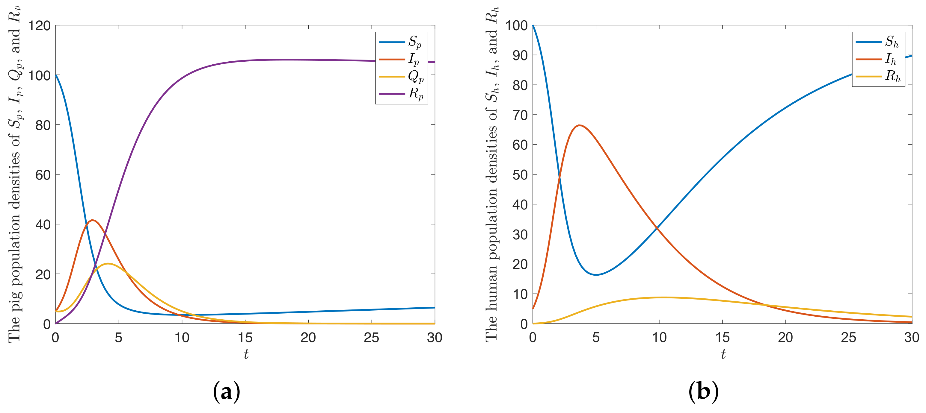
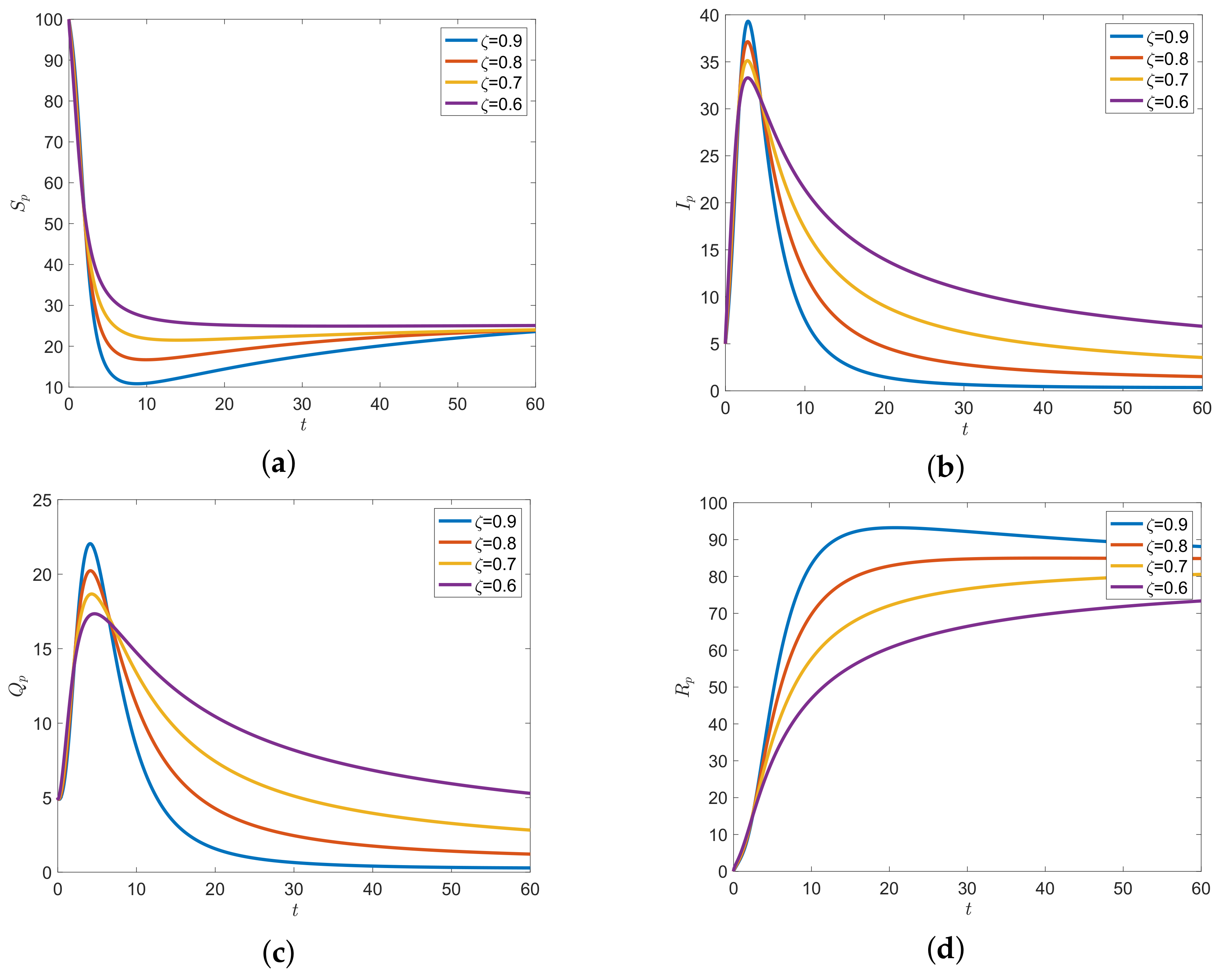
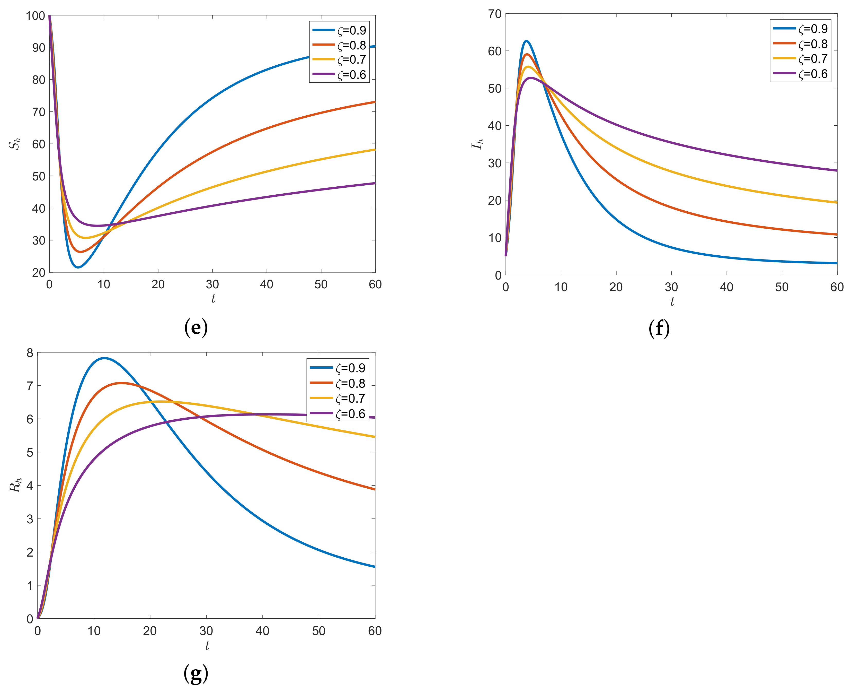
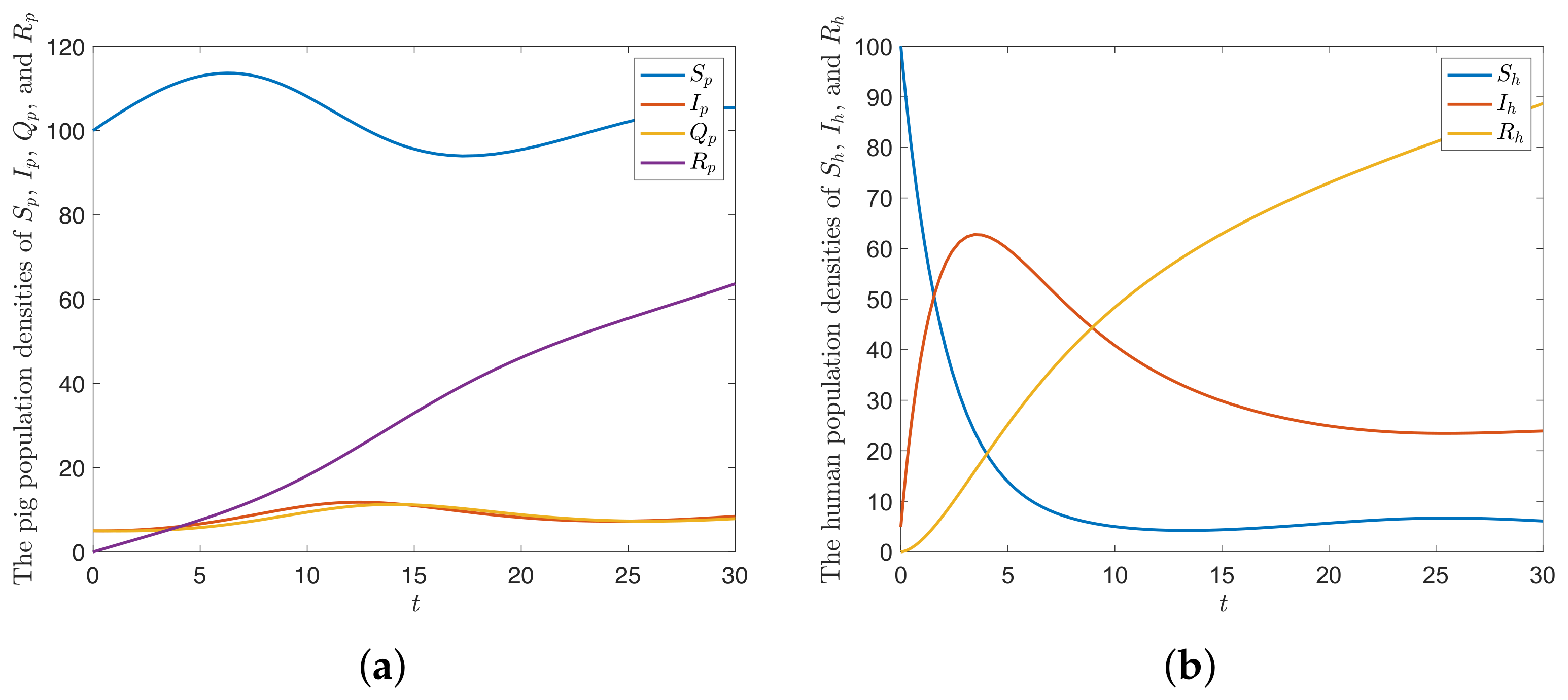
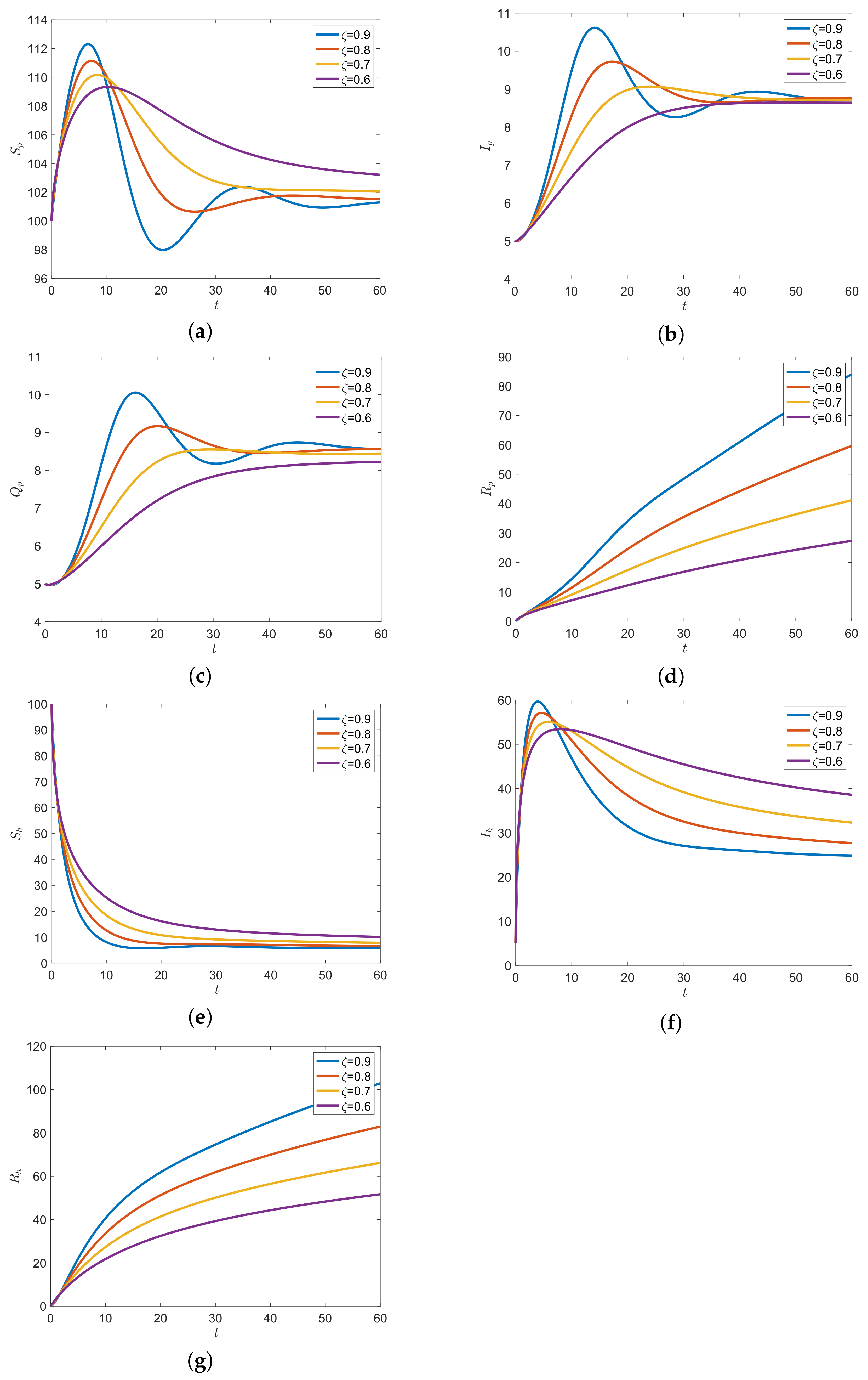
6.2. Numerical Examples

The numerical examples of the Atagana–Baleanu–Caputo fractional derivative system (7) are computed for demonstration of the disease transmission with the given initial values

$$S_p\left(0\right)=100,I_p\left(0\right)=5,Q_p\left(0\right)=5,R_p\left(0\right)=0,S_h\left(0\right)=100,I_h\left(0\right)=5,R_h\left(0\right)=0.$$

The parameter values of the numerical results of the integer-order model (9) are defined as $N_p=0.175,N_h=10,M=0.9,m=0.001,n=0.001,\delta =0.5,\epsilon =0.7,\alpha =0.1,$$\mu =0.1,\gamma =0.02,\beta =0.02,$ and ${\beta }_2=0.03$, which gives $R_0<1$. The trajectories of the solution approaches to disease-free equilibrium $\left(E_1\right)$, as shown in Figure 2.

The numerical simulation in Figure 2 shows that there are only pig susceptible, pig infected, human susceptible, and human infected populations at the beginning. After that, the disease spreads from the infected population to the susceptible population. The densities of pig- and human infected increase. Then, the densities of human infected and pig infected decrease to a lower value. The density of the pig quarantine class increases after the density of pig infected class increases, and then it decreases after the density of pig infected decreases. This means that the pig quarantine reduces the transmission of the disease. In the long run, the numerical results approached to the equilibrium point in the analysis part.

The parameter values of the numerical results of the ABC fractional order model (7) with various orders are defined as $N_p=0.175,N_h=10,M=0.9,m=0.001,n=0.001,$ $\delta =0.5,\epsilon =0.7,\alpha =0.1,\mu =0.1,\gamma =0.02,\beta =0.02,$ and ${\beta }_2=0.03$, which give $R_0<1$. The trajectories of the solution approaches to disease-free equilibrium $\left(E_1\right)$, as shown in Figure 3.

Figure 3 shows the solutions of the fractional order model with the ABC operator. The various values of the fractional order $\zeta =0.6,0.7,0.8,$ and $0.9$ were investigated. The results indicated that the fractional order provided different trajectories. This is the major benefit of the fractional order model. From a mathematical point of view, we can change the order of fractional order to find the best fit of the curve. In the long run, the numerical results show that higher fractional order provides the lower densities of all classes except human recovered classes. Then, the solution trajectories of all fractional orders leads to the disease-free equilibrium.

The parameter values of the numerical results of the integer-order model (9) are defined as $N_p=9,N_h=5,M=0.3,m=0.3,n=0.1,\delta =0.6,\epsilon =0.3,\alpha =0.1,$$\mu =0.01,$$\gamma =0.1,\beta =0.03,$ and ${\beta }_2=0.1$, which give $R_0>1$. The trajectories of the solution approaches to endemic equilibrium $\left(E_2\right)$, as shown in Figure 4.

The parameter values of the numerical results of the ABC fractional order model (7) with various orders are defined as $N_p=9,N_h=5,M=0.3,m=0.3,n=0.1,\delta =0.6,$$\epsilon =0.3,$$\alpha =0.1,\mu =0.01,\gamma =0.1,\beta =0.03,$ and ${\beta }_2=0.1$, which give $R_0<1$. The trajectories of the solution approaches to disease-free equilibrium $\left(E_2\right)$, as shown in Figure 5.

According to the numerical result in Figure 4, the solution trajectories lead to the endemic equilibrium when $R_0>1$. The endemic equilibrium is the state where the disease still transmits with constant densities in each class. Figure 5 shows that the solution trajectories of all classes have different values with different fractional-orders. Higher fractional orders provide lower densities for pig susceptible, pig infected, pig quarantine, and human susceptible. Otherwise, the higher fractional order provides higher densities for the pig removable, human infected, and human removable classes.

7. Conclusions

The dynamics of disease transmission for Streptococcus suis by considering the relation between humans and pigs is investigated. We have proposed the fractional order mathematical model based on the Atangana–Baleanu–Caputo fractional derivative. The proposed model is improved from the SIQR model, which can be expressed in the system of ordinary differential equations. The model is composed with seven compartments, these are the pig susceptible $\left(S_p\right)$, infectious $\left(I_p\right)$, quarantine $\left(Q_p\right)$, and recovery $\left(R_p\right)$ populations, and the human susceptible $\left(S_h\right)$, infectious $\left(I_h\right)$, and recovery $\left(R_h\right)$ populations. The proposed model has investigated the contact between pigs and humans. Many properties of the model have been investigated: the invariant region, equilibria, stability analysis, and the existence and uniqueness of the solution. The basic reproduction number $\left(R_0\right)$ of the model is also presented to explain the behavior of the disease. The conditions of equilibrium points are obtained. The disease-free equilibrium point is locally asymptotically stable if $R_0<1$. The endemic equilibrium is locally asymptotically stable if $R_0>1$. The numerical examples confirm the results from the proposed theorems, which lead the solution trajectories to the equilibria. Moreover, the fractional order derivative provides different solutions with the same parameters. Using the concept of the fractional order derivative, we can extend the mathematical models that are represented in the ordinary differential equation in this way.

References

1. Jones, K.E.; Patel, N.G.; Levy, M.A.; Storeygard, A.; Balk, D.; Gittleman, J.L.; Daszak, P. Global trends in emerging infectious diseases. Nature 2008, 451, 990–993. [Google Scholar] [CrossRef] [PubMed]
2. Li, F.; Du, L. MERS Coronavirus: An Emerging Zoonotic Virus. Viruses 2019, 11, 663. [Google Scholar] [CrossRef] [PubMed] [Green Version]
3. Mackenzie, J.S.; Smith, D.W. COVID-19: A novel zoonotic disease caused by a coronavirus from China: What we know and what we don’t. Microbiol. Aust. 2020, 41, 45–50. [Google Scholar] [CrossRef]
4. Gottschalk, M.; Xu, J.; Calzas, C.; Segura, M. Streptococcus suis: A new emerging or an old neglected zoonotic pathogen? Future Microbiol. 2010, 5, 371–391. [Google Scholar] [CrossRef] [PubMed]
5. Goyette-Desjardins, G.; Auger, J.; Xu, J.; Segura, M.; Gottschalk, M. Streptococcus suis, an important pig pathogen and emerging zoonotic agent—An update on the worldwide distribution based on serotyping and sequence typing. Emerg. Microbes Infect. 2014, 3, e45. [Google Scholar] [CrossRef] [PubMed]
6. Dutkiewicz, J.; Sroka, J.; Zajac, V.; Wasinski, B.; Cisak, E.; Sawczyn, A.; Kloc, A.; Wojcik-Fatla, A. Streptococcus suis: A re-emerging pathogen associated with occupational exposure to pigs or pork products. Part I—Epidemiology. Ann. Agric. Environ. Med. 2017, 24, 683–695. [Google Scholar] [CrossRef] [PubMed]
7. Feng, Y.; Zhang, H.; Wu, Z.; Wang, S.; Cao, M.; Hu, D.; Wang, C. Streptococcus suis infection. Virulence 2014, 5, 477–497. [Google Scholar] [CrossRef] [PubMed] [Green Version]
8. Gajdacs, M.; Nemeth, A.; Knausz, M.; Barrak, I.; Stajer, A.; Mestyan, G.; Melegh, S.; Nyul, A.; Toth, A.; Agoston, Z.; et al. Streptococcus suis: An Underestimated Emerging Pathogen in Hungary? Microorganisms 2020, 8, 1292. [Google Scholar] [CrossRef]
9. Lun, Z.R.; Wang, Q.P.; Chen, X.G.; Li, A.X.; Zhu, X.Q. Streptococcus suis: An emerging zoonotic pathogen. Lancet Infect. Dis. 2007, 7, 201–209. [Google Scholar] [CrossRef]
10. Huh, H.J.; Park, K.J.; Jang, J.H.; Lee, M.; Lee, J.H.; Ahn, Y.H.; Kang, C.I.; Ki, C.S.; Lee, N.Y. Streptococcus suis meningitis with bilateral sensorineural hearing loss. Korean J. Lab. Med. 2011, 31, 205–211. [Google Scholar] [CrossRef]
11. Hughes, J.M.; Wilson, M.E.; Wertheim, H.F.L.; Nghia, H.D.T.; Taylor, W.; Schultsz, C. Streptococcus suis: An Emerging Human Pathogen. Clin. Infect. Dis. 2009, 48, 617–625. [Google Scholar] [CrossRef] [Green Version]
12. Dekker, N.; Bouma, A.; Daemen, I.; Klinkenberg, D.; van Leengoed, L.; Wagenaar, J.A.; Stegeman, A. Effect of Spatial Separation of Pigs on Spread of Streptococcus suis Serotype 9. PLoS ONE 2013, 8, e61339. [Google Scholar] [CrossRef] [Green Version]
13. Hlebowicz, M.; Jakubowski, P.; Smiatacz, T. Streptococcus suis Meningitis: Epidemiology, Clinical Presentation and Treatment. Vector Borne Zoonotic Dis. 2019, 19, 557–562. [Google Scholar] [CrossRef]
14. Li, Z.; Xu, M.; Hua, X. Endogenous endophthalmitis caused by Streptococcus suis infection: A case report. BMC Ophthalmol. 2022, 22, 165. [Google Scholar] [CrossRef]
15. Okura, M.; Osaki, M.; Nomoto, R.; Arai, S.; Osawa, R.; Sekizaki, T.; Takamatsu, D. Current Taxonomical Situation of Streptococcus suis. Pathogens 2016, 5, 45. [Google Scholar] [CrossRef] [Green Version]
16. Giang, E.; Hetman, B.M.; Sargeant, J.M.; Poljak, Z.; Greer, A.L. Examining the Effect of Host Recruitment Rates on the Transmission of Streptococcus suis in Nursery Swine Populations. Pathogens 2020, 9, 174. [Google Scholar] [CrossRef] [Green Version]
17. Oishi, K.; Dejsirilert, S.; Puangpatra, P.; Sripakdee, S.; Chumla, K.; Boonkerd, N.; Polwichai, P.; Tanimura, S.; Takeuchi, D.; Nakayama, T.; et al. Genotypic Profile of Streptococcus suis Serotype 2 and Clinical Features of Infection in Humans, Thailand. Emerg. Infect. Dis. 2011, 17, 835–842. [Google Scholar] [CrossRef]
18. Zhu, Y.; Zhu, F.; Bo, L.; Fang, Y.; Shan, X. A rare case of meningitis and septicemia caused by Streptococcus suis in a woman without a history of live pig contact or eating raw pork. Braz. J. Microbiol. 2021, 52, 2007–2012. [Google Scholar] [CrossRef]
19. Takeuchi, D.; Kerdsin, A.; Pienpringam, A.; Loetthong, P.; Samerchea, S.; Luangsuk, P.; Khamisara, K.; Wongwan, N.; Areeratana, P.; Chiranairadul, P.; et al. Population-Based Study of Streptococcus suis Infection in Humans in Phayao Province in Northern Thailand. PLoS ONE 2012, 7, e31265. [Google Scholar] [CrossRef] [Green Version]
20. Takeuchi, D.; Kerdsin, A.; Akeda, Y.; Chiranairadul, P.; Loetthong, P.; Tanburawong, N.; Areeratana, P.; Puangmali, P.; Khamisara, K.; Pinyo, W.; et al. Impact of a Food Safety Campaign on Streptococcus suis Infection in Humans in Thailand. Am. Soc. Trop. Med. Hyg. 2017, 96, 1370–1377. [Google Scholar] [CrossRef]
21. Jiang, F.; Guo, J.; Cheng, C.; Gu, B. Human infection caused by Streptococcus suis serotype 2 in China: Report of two cases and epidemic distribution based on sequence type. BMC Infect. Dis. 2020, 20, 223. [Google Scholar] [CrossRef] [Green Version]
22. Dattner, I.; Huppert, A. Modern statistical tools for inference and prediction of infectious diseases using mathematical models. Stat. Methods Med. Res. 2018, 27, 1927–1929. [Google Scholar] [CrossRef] [Green Version]
23. Adekola, H.A.; Adekunle, I.A.; Egberongbe, H.O.; Onitilo, S.A.; Abdullahi, I.N. Mathematical modeling for infectious viral disease: The COVID-19 perspective. J. Public Aff. 2020, 20, e2306. [Google Scholar] [CrossRef]
24. Prathumwan, D.; Trachoo, K.; Chaiya, I. Mathematical Modeling for Prediction Dynamics of the Coronavirus Disease 2019 (COVID-19) Pandemic, Quarantine Control Measures. Symmetry 2020, 12, 1404. [Google Scholar] [CrossRef]
25. Chamnan, A.; Pongsumpun, P.; Tang, I.M.; Wongvanich, N. Local and Global Stability Analysis of Dengue Disease with Vaccination and Optimal Control. Symmetry 2021, 13, 1917. [Google Scholar] [CrossRef]
26. Fatmawati; Jan, R.; Khan, M.A.; Khan, Y.; Ullah, S. A new model of dengue fever in terms of fractional derivative. Math. Biosci. Eng. 2020, 17, 5267–5287. [Google Scholar] [CrossRef]
27. Huang, Y.; Li, J.; Zhang, J.; Jin, Z. Dynamical analysis of the spread of African swine fever with the live pig price in China. Math. Biosci. Eng. 2021, 18, 8123–8148. [Google Scholar] [CrossRef]
28. Carvalho, S.A.; da Silva, S.O.; Charret, I.d.C. Mathematical modeling of dengue epidemic: Control methods and vaccination strategies. Theory Biosci. 2019, 138, 223–239. [Google Scholar] [CrossRef] [Green Version]
29. Kumar, P.; Baleanu, D.; Erturk, V.S.; Inc, M.; Govindaraj, V. A delayed plant disease model with Caputo fractional derivatives. Adv. Contin. Discret. Model. 2022, 2022, 11. [Google Scholar] [CrossRef]
30. Peter, O.J.; Shaikh, A.S.; Ibrahim, M.O.; Nisar, K.S.; Baleanu, D.; Khan, I.; Abioye, A.I. Analysis and Dynamics of Fractional Order Mathematical Model of COVID-19 in Nigeria Using Atangana-Baleanu Operator. Comput. Mater. Contin. 2021, 66, 1823–1848. [Google Scholar] [CrossRef]
31. Shen, C.; Li, M.; Zhang, W.; Yi, Y.; Wang, Y.; Hou, Q.; Huang, B.; Lu, C. Modeling Transmission Dynamics of Streptococcus suis with Stage Structure and Sensitivity Analysis. Discret. Dyn. Nat. Soc. 2014, 2014, 432602. [Google Scholar] [CrossRef] [Green Version]
32. Podlubny, I. Fractional Differential Equations. Mathematics in Science and Engineering; Academic Press: San Diego, CA, USA, 1999. [Google Scholar]
33. Atangana, A.; Baleanu, D. New fractional derivatives with non-local and non-singular kernel: Theory and application to heat transfer model. Therm. Sci. 2016, 20, 763–769. [Google Scholar] [CrossRef] [Green Version]
34. Lipsitch, M.; Nowak, M.A.; Ebert, D.; May, R.M. The population dynamics of vertically and horizontally transmitted parasites. Proc. R. Soc. Lond. Ser. B Biol. Sci. 1995, 260, 321–327. [Google Scholar] [CrossRef]
35. Naresh, R.; Tripathi, A.; Omar, S. Modelling the spread of AIDS epidemic with vertical transmission. Appl. Math. Comput. 2006, 178, 262–272. [Google Scholar] [CrossRef]
36. van den Driessche, P.; Watmough, J. Reproduction numbers and sub-threshold endemic equilibria for compartmental models of disease transmission. Math. Biosci. 2002, 180, 29–48. [Google Scholar] [CrossRef]
37. Diekmann, O.; Heesterbeek, J.A.P.; Roberts, M.G. The construction of next-generation matrices for compartmental epidemic models. J. R. Soc. Interface 2010, 7, 873–885. [Google Scholar] [CrossRef] [Green Version]
38. Gupta, P.K.; Dutta, A. A mathematical model on HIV/AIDS with fusion effect: Analysis and homotopy solution. Eur. Phys. J. Plus 2019, 134, 265. [Google Scholar] [CrossRef]
39. Goodrich, C.S. Existence of a positive solution to a class of fractional differential equations. Appl. Math. Lett. 2010, 23, 1050–1055. [Google Scholar] [CrossRef] [Green Version]
40. Sinan, M.; Ahmad, H.; Ahmad, Z.; Baili, J.; Murtaza, S.; Aiyashi, M.; Botmart, T. Fractional mathematical modeling of malaria disease with treatment & insecticides. Results Phys. 2022, 34, 105220. [Google Scholar] [CrossRef]
Figure 1. The compartmental diagram for disease transmission dynamics of S. Suis infection for pigs and humans.
Symmetry 14 02112 g001
Figure 2. The trajectories of the solution of the model SIQR-SIR approaching to E 1 when R 0 < 1 for (a) pig population (b) human population.
Symmetry 14 02112 g002
Figure 3. The solution trajectories of the system (7) when R 0 < 1 for (a) pig susceptible class, (b) pig infectious class, (c) pig quarantine class, (d) pig removable class, (e) human susceptible class, (f) human infectious class, and (g) human removable class with various time fractional orders ζ = 0.6 , 0.7 , 0.8 , and 0.9 .
Symmetry 14 02112 g003aSymmetry 14 02112 g003b
Figure 4. The trajectories of the solution of the model SIQR-SIR approaching to E 2 when R 0 > 1 for (a) pig population (b) human population.
Symmetry 14 02112 g004
Figure 5. The solution trajectories of the system (7) when R 0 > 1 for (a) pig susceptible class, (b) pig infectious class, (c) pig quarantine class, (d) pig removable class, (e) human susceptible class, (f) human infectious class, and (g) human removable class with various time fractional orders ζ = 0.6 , 0.7 , 0.8 , and 0.9 .
Symmetry 14 02112 g005
Publisher’s Note: MDPI stays neutral with regard to jurisdictional claims in published maps and institutional affiliations.