Novel Distance-Measures-Based Extended TOPSIS Method under Linguistic Linear Diophantine Fuzzy Information

Abstract

The advantages of the intuitionistic fuzzy set, Pythagorean fuzzy set, and q-rung orthopair fuzzy set are all carried over into the linear Diophantine fuzzy set by extending the restrictions on the grades. Linear Diophantine fuzzy sets offer a wide range of practical applications because the reference parameters allow evaluation andto express their judgments about membership and nonmembership degrees in a variety of ways. Linguistic-valued information cannot be described by linear Diophantine fuzzy numbers since precise numbers are used in linear Diophantine fuzzy systems. In this paper, we first present the novel idea of a linguistic linear Diophantine fuzzy set, which is the hybrid structure of the linear Diophantine fuzzy set and the linguistic term set. Furthermore, some basic operational rules with novel distance measures, namely, Hamming, Euclidean, and Chebyshev distance measures, are established. Based on the newly defined concept of distance measure, an extended TOPSIS technique is presented to tackle the linguistic uncertainty in real-world decision support problems. A numerical example is illustrated to support the applicability of the proposed methodology and to analyze symmetry of the optimal decision. A comparison analysis is constructed to show the symmetry, validity, and effectiveness of the proposed method over the existing decision support techniques.

1. Introduction

The fuzzy set, which was first developed by Zadeh in 1965 [1], has had considerable success in a number of different domains and is regarded as a useful tool for decision-making, medical diagnosis, pattern recognition, and fuzzy inference (Cateni, S., Colla, V., & Nastasi, G. (2013) [2]; Das et al., 2016 [3]; Yager, 1977 [4]). The fuzzy set has been extended in several ways since it was first introduced. The intuitionistic fuzzy set (IFS), developed by Atanassov, is one of a fuzzy set’s generalizations (1986) [5]. The membership and nonmembership functions can be stated as the grade of satisfactory and unsatisfactory, respectively, which is a typical aspect of IFS. The sum of the membership degree and the nonmembership degree must, however, be equal to or lower than one, according to IFSs. Some information related to decision evaluation cannot be successfully communicated in this situation due to the possibility that certain decision-makers may supply information for an attribute where the total of membership degree and nonmembership degree is more than one. As a result, to address these issues, Yager (2013) [6] proposed the idea of a Pythagorean fuzzy set (PyFS), which has the distinguishing characteristic that the square sum of the grade of membership and grade of nonmembership is less than or equal to one. With the development of PyFS theory, considering the complexity of the problems, a new concept was described again by Yager (2017) [7], the q-rung orthopair fuzzy set (q-ROFS), where the sum of the qth power $(q\ge 1)$ of membership degree and nonmembership degree is restricted to one. It can be seen that q-ROFs are general because IFSs and PyFSs are their special cases. Many authors have studied them extensively and deeply; these studies mainly include the following aspects: (1) the basic theory research, such as operational laws (Peng & Luo, 2021 [8]; Rahman et al., 2017 [9]), similarity and distance measures (Ejegwa, 2020 [10]; Farhadinia et al., 2021 [11]; Garg, (2018a) [12]; Hussian et al., (2019) [13]), (2) some extended multicriteria decision-making (MCDM) methods (Aydemir & Gunduz, 2019; Biswas, & Deb, 2021; Büyüközkan et al., 2021; Ejegwa, 2019, Jana et al., 2019), (3) aggregation operators research (Aydemir, & Gunduz, 2019 [14]; Biswas, & Deb, (2021) [15]; Jana et al., (2019) [16]), and so on. Akram et al. (2022) [17] proposed a new combined model of complex Fermatean fuzzy N-soft set, and Feng el al. (2022) [18] proposed a new SF for ranking order of q-ROFNs for MADM. Karaaslan and Cagman (2022) [19] developed some similarity measures with parameter trees based on soft set theory.

According to Riaz and Hashmi (2019) [20], these set theories have restrictions in relation to membership and nonmembership degrees. They suggested the use of reference/control parameters along with a linear Diophantine fuzzy set (LDFS) to remove these restrictions. Riaz et al. (2019; 2020) and Ayub et al. (2021) [21] argued that LDFS is more flexible and reliable than existing concepts of IFSs, PFSs, and q-ROFSs. In 2021, Kamacı et al. [22,23] studied the theoretical aspects and complex types of LDFSs. Due to the advantages of LDFS in practice, they attracted the attention of many researchers in different scientific fields, and many seminal articles were published (Almagrabi et al., 2021 [24]; Izmand et al., 2021 [25]; Mahmood et al., 2021 [26]). The research on other generalizations of a fuzzy set has been growing rapidly (Ashraf et al., 2019 [27]; Cuong, 2014 [28]; Kamacı et al., 2021a, 2021b [29,30]). Decision support systems in real-life scenarios can be seen (Deveci et al., 2022a; 2022b [31,32]).

Real-world problems are fuzzy and unpredictable, making it challenging to give qualitative evaluation using accurate values. People frequently express their ideas at this period using linguistic words. In some real-world situations, evaluators treat linguistic data as the values of linguistic variables; that is, the variables’ values are expressed linguistically, rather than numerically, using terms such as “very awful”, “bad”, “fair”, “better”, “good”, and “somewhat good”. The concept of linguistic variables was first developed by Zadeh (1975 [33]), who then concentrated on its usage in fuzzy reasoning to describe information that cannot be represented by precise numbers. Based on linguistic evaluations, Herrera et al. (1996a, 1996b, 2000 [34,35,36]) suggested some consensus models for group decision-making. Additionally, linguistic ordered weighted geometric operator and linguistic hybrid aggregation operator were developed by Xu (2014, 2015 [37,38]), who subsequently used them to solve multiple attribute group decision-making problems including linguistic information. Some authors studied multi-bijective linguistic decision systems (Gong et al., 2010 [39]). Rodríquez et al., (2021) [40] and Yu et al., (2017 [41]) focused on the fuzzy linguistic term sets and their applications in handling multicriteria decision-making. The linguistic intuitionistic fuzzy numbers (LIFNs) and linguistic intuitionistic fuzzy sets (LIFSs) were characterized by deriving the language forms of intuitionistic fuzzy variables (Chen et al., 2015 [42]; Ou et al., 2018 [43]; Zhang, 2014 [44]). In recent years, many researchers focused on the aggregation operators (AOs) of LIFNs, such as power AOs (Garg, & Kumar, 2019 [45]; Liu, & Qin, 2017 [46]; Liu, & Wang, 2017 [47]), Einstein AOs (Garg, & Kumar, 2018 [48]), Heronian AOs (Liu et al., 2014 [49]), and Bonferroni AOs (Wei et al., 2013 [50]). Later, Garg (2018b [51]) proposed an extended form of the LIFS which is called the linguistic Pythagorean fuzzy set (LPyFS). There are many papers in the literature related to LDFSs [52]. Lin et al. (2020 [53]) investigated the difference between LIFS and LPyFS, and then initiated the theory of linguistic q-rung orthopair fuzzy set (Lq-ROFS), which loosened the existing constraints for linguistic membership and nonmembership degrees in the structures of LIFS and LPyFS. For more linguistic fuzzy approaches, see (Jin et al., 2019 [54]; Liu et al., 2020 [55]). Some extensive work related to different extensions of fuzzy sets can be seen in (Deveci et al., 2022c; 2022d; 2022e [56,57,58]). Ali et al. [59] and Ashraf et al. [60] proposed some AOs for interval-valued picture fuzzy set. Kazemitash et al. [61] and Bozanic et al. [62] gave some ideas related to some different extensions of fuzzy set. For other terminologies not discussed in the paper, the readers are referred to [63,64,65].

The prevalent theories of LIFS, LPyFS, and Lq-ROFS have many applications in a variety of real-world contexts, but they also have some drawbacks connected to linguistic membership and nonmembership grades. With the addition of reference parameters that are expressed in linguistic terms, we develop the novel idea of the linguistic linear Diophantine fuzzy set (LLDFS) to remove these limitations. Due to the usage of linguistic-valued reference parameters, the suggested notion of LLDFS is more effective and adaptable than other linguistic fuzzy techniques. Additionally, LDFS models under linguistic information can likewise be applied to LLDFS models. By altering the physical meaning of membership, nonmembership, and reference parameters in the structure of LDFS, we may state that LLDFS categorizes the data in linguistic multicriteria decision-making (LMCDM) situations. With the use of linguistic reference/control parameters, this set widens the space for linguistic membership and nonmembership degrees, covering the spaces of the linguistic fuzzy structures previously stated. The following list includes some of this paper’s key points.

(1)

More broadly applicable than LIFS, LPyFS, and Lq-ROFS are the theories of LLDFS.

(2)

The idea of LLDFS makes it possible to express, in language terms, the degrees of membership and nonmembership as well as the reference parameters found in the structure of LDFSs. As a result, it can handle decision-making based on LDFS with regard to linguistic information.

(3)

In some real-life problems, the sum of linguistic-valued degrees of membership and nonmembership to which an alternative satisfying an attribute provided by the decision-maker (DM) may be larger than g, where $g+1$ is the number of elements of the linguistic term set, and their sum of squares is also larger than $g^2$. The LIFS and LPyFS fail in such situations. To overcome these shortcomings, Lq-ROFS is proposed, using the condition that the sum of the qth power ($q\ge 1$) of linguistic membership degree and linguistic nonmembership degree is limited to the interval $[0,g^q]$. In some practical problems, both the linguistic membership degree and the linguistic nonmembership degree may be equal to g, which contradicts the constraint of Lq-ROFS. LLDFS can deal with such situations, and thus provides a large number of applications to the LMCDM for such real-life problems.

(4)

The proposed model and LMCDM issues are shown to be closely related. This link leads to the construction of a modified TOPSIS algorithm to handle uncertainty in multi-attribute data in a parametric way. LMCDM issues are satisfactorily solved by the linguistic linear Diophantine fuzzy TOPSIS (LLDF-TOPSIS) approach, which enhances the TOPSIS methods based on LIFSs, LPyFSs, and Lq-ROFSs.

The rest of the paper is organized as follows. In Section 2, some basic concepts of linguistic term set and LDFS are briefly reviewed. In Section 3, we introduce the concept of LLDFS and discuss their basic operational laws, weighted aggregation operators, and score functions. Section 4 presents some formulas to measure the distance between two linguistic linear Diophantine fuzzy numbers (LLDFNs). Section 5 proposes a modified TOPSIS procedure to deal with LMCDM under the LLDF environment. To determine the consistency and validity of the elaborated LLDF-TOPSIS, an illustrative example is given that selects the best software consultants. Finally, the sensitivity analysis, comparison analysis, and merits of the proposed LLDF-TOPSIS method are also discussed. The conclusions are given in Section 6.

2. Preliminaries

This section reviews some related concepts to facilitate the discussions in the next sections.

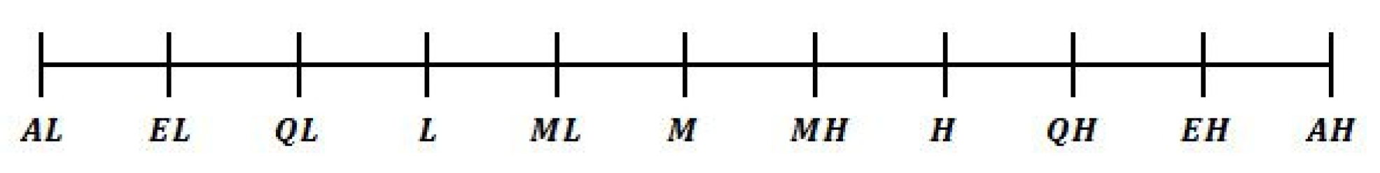
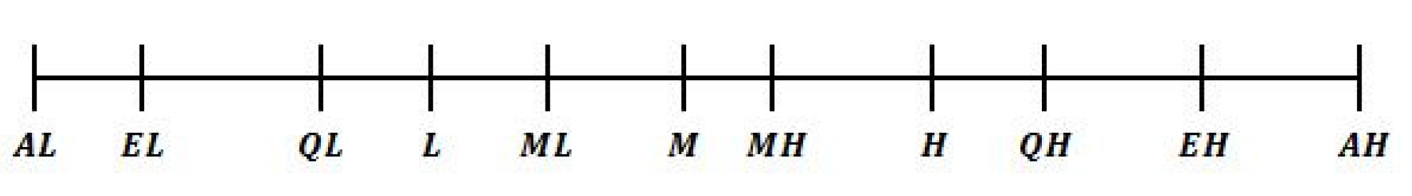
2.1. Linguistic Term Set

The linguistic approach is an approximate technique that represents qualitative aspects as linguistic values by means of linguistic variables.

Definition 1

(Herrera et al., 1996a, 2000 [34,35]). The set $Ł=\{{ł}_0,{ł}_1,\dots ,{ł}_g\}$ is called a (finite) linguistic term set with odd cardinality $g+1$, where ${ł}_{\kappa }$ represents a possible value of a linguistic variable. The linguistic terms should satisfy the following characteristics:

(1) 

The order relation: ${ł}_{\kappa }\ge {ł}_{\tau }$ if $\kappa \ge \tau$;

(2) 

The negation operator: $neg\left({ł}_{\kappa }\right)={ł}_{g-\kappa }$;

(3) 

The max (maximization) operator: $max\{{ł}_{\kappa },{ł}_{\tau }\}={ł}_{\kappa }$ if ${ł}_{\kappa }\ge {ł}_{\tau }$;

(4) 

The min (minimization) operator: $min\{{ł}_{\kappa },{ł}_{\tau }\}={ł}_{\kappa }$ if ${ł}_{\kappa }\le {ł}_{\tau }$.

Example 1.

For $g=10$,

$$\begin{array}{c}\hfill Ł=\left\{\begin{array}{c}{ł}_0=AbsolutelyLow\left(AL\right),{ł}_1=ExtremelyLow\left(EL\right),{ł}_2=QuiteLow\left(QL\right),{ł}_3=Low\left(L\right),\hfill \\ {ł}_4=MildlyLow\left(ML\right),{ł}_5=Medium\left(M\right),{ł}_6=MildlyHigh\left(MH\right),{ł}_7=High\left(H\right),\hfill \\ {ł}_8=QuiteHigh\left(QH\right),{ł}_9=ExtremelyHigh\left(EH\right),{ł}_{10}=AbsolutelyHigh\left(AH\right)\hfill \end{array}\right\}\end{array}$$

is a linguistic term set. The cardinality of this set is $g+1=11$.

Considering the set Ł in Example 1, the symmetrical and nonsymmetrical distributions of the eleven linguistic labels of this linguistic term set can be presented as in Figure 1 and Figure 2, respectively.

To preserve all the given information, Xu (2004 [37]) extended discrete linguistic term set Ł to a continuous linguistic term set.

Definition 2

(Xu, 2004 [37]). Let $Ł=\{{ł}_0,{ł}_1,\dots ,{ł}_g\}$ be a linguistic term set with odd cardinality $g+1$. Then, ${Ł}_{[0,g]}=\{{ł}_{\kappa }:{ł}_0\le {ł}_{\kappa }\le {ł}_g,\kappa \in [0,g]\}$ is an extended form of and it is termed to be a continuous linguistic term set for Ł.

If ${ł}_{\kappa }\in Ł$, then ${ł}_{\kappa }$ is termed to be the original linguistic term, otherwise ${ł}_{\kappa }$ is said to be the virtual linguistic term (Xu, 2004 [37]).

Example 2.

Consider the linguistic term set Ł in Example 1. ${Ł}_{[0,10]}=\{{ł}_{\kappa }:{ł}_0\le {ł}_{\kappa }\le {ł}_{10},\kappa \in [0,10]\}$ is a continuous linguistic term set for Ł. For example, ${ł}_7\in Ł$ is an original linguistic term, but ${ł}_{7.4}\notin Ł$ (${ł}_{7.4}\in {Ł}_{[0,10]}$) is a virtual linguistic term and it can be considered as the corresponding degree between high (H) and quite high (QH).

2.2. Linear Diophantine Fuzzy Set

Riaz and Hashmi (2019 [20]) emphasized that while the theories of IFSs, PyFSs, and q-ROFSs are excellent tools in handling multicriteria decision-making problems where alternatives are evaluated by an expert(s) according to the choice parameters, they cannot deal with multicriteria decision-making problems where alternatives are evaluated by an expert(s) according to the choice parameters controlled by the reference parameters. Thus, they argued that the theories of IFSs, PyFSs, and q-ROFSs have their limitations related to the membership degree and nonmembership degree. To remove these restrictions, they proposed the idea of LDFS by integrating reference/control parameters into the structures of IFS, PyFS, and q-ROFS. Moreover, they proposed that considering the special cases of reference parameters, it is obvious that LDFSs are the more general forms of FSs, IFSs, PyFSs, and q-ROFSs. Therefore, LDFS-based decision-making methods can deal with multicriteria decision-making problems under the environments of FSs, IFS, PyFS, and q-ROFS. The definition of LDFS is as follows.

Throughout this paper, $\mathcal{H}=\{{\hslash }_i:i=1,2,\dots ,s\}$ denotes the universal discourse set.

Definition 3

(Riaz, & Hashmi, 2019 [20]). An LDFS D in $\mathcal{H}$ is described as

$$\begin{array}{c}\hfill D=\{({\hslash }_i,\langle {\Psi }_D\left({\hslash }_i\right),{\Theta }_D\left({\hslash }_i\right)\rangle ,\langle {\rho }_D\left({\hslash }_i\right),{\sigma }_D\left({\hslash }_i\right)\rangle ):{\hslash }_i\in \mathcal{H}\}\end{array}$$

(1)

where ${\psi }_D\left({\hslash }_i\right),{\Theta }_D\left({\hslash }_i\right),{\rho }_D\left({\hslash }_i\right),{\sigma }_D\left({\hslash }_i\right)\in [0,1]$, respectively, represent the degrees of membership, nonmembership, and reference/control parameters of ${\hslash }_i\in \mathcal{H}$ into the set D. These degrees fulfill the constraint

$$\begin{array}{c}\hfill 0\le {\rho }_D\left({\hslash }_i\right)+{\sigma }_D\left({\hslash }_i\right)\le 1\mathrm{and}0\le {\rho }_D\left({\hslash }_i\right){\Psi }_D\left({\hslash }_i\right)+{\sigma }_D\left({\hslash }_i\right){\Theta }_D\left({\hslash }_i\right)\le 1.\end{array}$$

for all ${\hslash }_i\in \mathcal{H}$. The hesitation margin of each ${\hslash }_i\in \mathcal{H}$ is ${\pi }_D\left({\hslash }_i\right){\Phi }_D\left({\hslash }_i\right)=1-({\rho }_D\left({\hslash }_i\right){\Psi }_D\left({\hslash }_i\right)+{\sigma }_D\left({\hslash }_i\right){\Theta }_D\left({\hslash }_i\right))$, where ${\pi }_D$ is the reference/control parameter related to the degree of hesitancy. Simply, $\aleph =(\langle {\Psi }_D,{\Theta }_D\rangle ,\langle {\rho }_D,{\sigma }_D\rangle )$ is named linear Diophantine fuzzy number (LDFN) with $0\le {\rho }_D+{\sigma }_D\le 1$ and $0\le {\rho }_D{\Psi }_D+{\sigma }_D{\Theta }_D\le 1$.

Example 3.

Let $\mathcal{H}=\{{\hslash }_i:i=1,2,\dots ,5\}$ be a collection of some life-saving drugs. Let us define the following notions.

$$\begin{array}{cc}\hfill {\Psi }_D(\hslash )& =Membershipgrade.\hfill \\ \hfill {\Theta }_D(\hslash )& =Nonmembershipgrade.\hfill \\ \hfill {\rho }_D(\hslash )& =Goodimpactagainstinfection.\hfill \\ \hfill {\sigma }_D(\hslash )& =Notgoodimpactagainstinfection.\hfill \end{array}$$

Then, its LDFS is given in

Table 1. LDFS for medication.

Alternatives	LDFNs
${\hslash }_1$	$\left(\right(0.639,0.573),$$(0.671,0.312))$
${\hslash }_2$	$\left(\right(0.867,0.514),$$(0.629,0.234))$
${\hslash }_3$	$\left(\right(0.657,0.867),$$(0.364,0.145))$
${\hslash }_4$	$\left(\right(0.678,0.787),$$(0.243,0.215))$
${\hslash }_5$	$\left(\right(0.876,0.767),$$(0.4245,0.342))$

.

Further, Riaz and Hasmi (2019) described some operational rules for the LDFNs as follows:

Let $\aleph =(\langle {\Psi }_D,{\Theta }_D\rangle ,\langle {\rho }_D,{\sigma }_D\rangle )$, ${\aleph }_1=(\langle {}^1{\Psi }_D,{}^1{\Theta }_D\rangle ,\langle {}^1{\rho }_D,{}^1{\sigma }_D\rangle )$ and

${\aleph }_2=(\langle {}^2{\Psi }_D,{}^2{\Theta }_D\rangle ,\langle {}^2{\rho }_D,{}^2{\sigma }_D\rangle )$ be three LDFNs in D and $\varpi >0$. Then,

• ${\aleph }_1\subseteq {\aleph }_2\iff$${}^1{\Psi }_D\le {}^2{\Psi }_D$, ${}^1{\Theta }_D\ge {}^2{\Theta }_D$, ${}^1{\rho }_D\le {}^2{\rho }_D$ and ${}^1{\sigma }_D\ge {}^2{\sigma }_D$;
• ${\aleph }_1={\aleph }_2\iff$${}^1{\Psi }_D={}^2{\Psi }_D$, ${}^1{\Theta }_D={}^2{\Theta }_D$, ${}^1{\rho }_D={}^2{\rho }_D$ and ${}^1{\sigma }_D={}^2{\sigma }_D$;
• ${\aleph }^c=(\langle {\Theta }_D,{\Psi }_D\rangle ,\langle {\sigma }_D,{\rho }_D\rangle )$;
• ${\aleph }_1\cup {\aleph }_2=(\langle sup{\{}^1{\Psi }_D,{}^2{\Psi }_D\},inf{\{}^1{\Theta }_D,{}^2{\Theta }_D\}\rangle ,\langle sup{\{}^1{\rho }_D,{}^2{\rho }_D\},inf{\{}^1{\sigma }_D,{}^2{\sigma }_D\}\rangle )$;
• ${\aleph }_1\cap {\aleph }_2=(\langle inf{\{}^1{\Psi }_D,{}^2{\Psi }_D\},sup{\{}^1{\Theta }_D,{}^2{\Theta }_D\}\rangle ,\langle inf{\{}^1{\rho }_D,{}^2{\rho }_D\},sup{\{}^1{\sigma }_D,{}^2{\sigma }_D\}\rangle )$;
• ${\aleph }_1\oplus {\aleph }_2=({\langle }^1{\Psi }_D+{}^2{\Psi }_D-{}^1{\Psi }_D{}^2{\Psi }_D{,}^1{\Theta }_D{}^2{\Theta }_D\rangle ,{\langle }^1{\rho }_D+{}^2{\rho }_D{-}^1{\rho }_D{}^2{\rho }_D{,}^1{\sigma }_D{}^2{\sigma }_D\rangle )$;
• ${\aleph }_1\otimes {\aleph }_2=({\langle }^1{\Psi }_D{}^2{\Psi }_D{,}^1{\Theta }_D+{}^2{\Theta }_D-{}^1{\Theta }_D{}^2{\Theta }_D\rangle ,{\langle }^1{\rho }_D{}^2{\rho }_D{,}^1{\sigma }_D+{}^2{\sigma }_D{-}^1{\sigma }_D{}^2{\sigma }_D\rangle )$;
• $\gamma \aleph =(\langle 1-{(1-{\Psi }_D)}^{\gamma },{\Theta }_D^{\gamma }\rangle ,\langle 1-{(1-{\rho }_D)}^{\gamma },{\sigma }_D^{\gamma }\rangle )$;
• ${\aleph }^{\gamma }=(\langle {\Psi }_D^{\gamma },1-{(1-{\Theta }_D)}^{\gamma }\rangle ,\langle {\rho }_D^{\gamma },1-{(1-{\sigma }_D)}^{\gamma }\rangle )$.

3. Linguistic Linear Diophantine Fuzzy Sets

3.1. Construction of Linguistic Linear Diophantine Fuzzy Set

In some complex situations (especially for some qualitative arguments), it is difficult for one to give the degrees of membership, nonmembership, and reference/control parameters with real numbers. A practicable solution is to express them by linguistic arguments. Based on this idea, we can propose the LLDF concepts to express the LDF information based on linguistic variables. In this part, we propose an LLDFS, whose degrees of membership, nonmembership, and reference/control parameters are represented by linguistic variables.

In real life, we occasionally encounter some problems in which the LDF information cannot be expressed by real numbers, that is, the LDF information we collect is qualitative. To describe the LDF information based on linguistic variables, the concept of the LLDFS is defined as follows.

Definition 4.

Let $Ł=\{{ł}_0,{ł}_1,\dots ,{ł}_g\}$ be a linguistic term set with odd cardinality $q+1$ and ${Ł}_{[0,g]}=\{{ł}_{\kappa }:{ł}_0\le {ł}_{\kappa }\le {ł}_g,\kappa \in [0,g]\}$. Then, an LLDFS $\mathfrak{D}$ in $\mathcal{H}$ is defined as

$$\begin{array}{c}\hfill \mathfrak{D}=\{({\hslash }_i,\langle {ł}_{{\Psi }_{\mathfrak{D}}}\left({\hslash }_i\right),{ł}_{{\Theta }_{\mathfrak{D}}}\left({\hslash }_i\right)\rangle ,\langle {ł}_{{\rho }_{\mathfrak{D}}}\left({\hslash }_i\right),{ł}_{{\sigma }_{\mathfrak{D}}}\left({\hslash }_i\right)\rangle ):{\hslash }_i\in \mathcal{H}\}\end{array}$$

(2)

where ${ł}_{{\Psi }_{\mathfrak{D}}}\left({\hslash }_i\right),{ł}_{{\Theta }_{\mathfrak{D}}}\left({\hslash }_i\right),{ł}_{{\rho }_{\mathfrak{D}}}\left({\hslash }_i\right),{ł}_{{\sigma }_{\mathfrak{D}}}\left({\hslash }_i\right)\in {Ł}_{[0,g]}$ represent the linguistic-valued degrees of membership, nonmembership, and reference/control parameters of ${\hslash }_i$ into $\mathfrak{D}$, respectively, with conditions for every ${\hslash }_i\in \mathcal{H}$,

$$\begin{array}{c}\hfill 0\le {\rho }_{\mathfrak{D}}\left({\hslash }_i\right)+{\sigma }_{\mathfrak{D}}\left({\hslash }_i\right)\le g\mathrm{and}0\le {\rho }_{\mathfrak{D}}\left({\hslash }_i\right){\Psi }_{\mathfrak{D}}\left({\hslash }_i\right)+{\sigma }_{\mathfrak{D}}\left({\hslash }_i\right){\Theta }_{\mathfrak{D}}\left({\hslash }_i\right)\le g^2.\end{array}$$

where $0\le {\Psi }_{\mathfrak{D}}\left({\hslash }_i\right),{\Theta }_{\mathfrak{D}}\left({\hslash }_i\right),{\rho }_{\mathfrak{D}}\left({\hslash }_i\right),{\sigma }_{\mathfrak{D}}\left({\hslash }_i\right)\le g$. Moreover, $(\langle {ł}_{{\Psi }_{\mathfrak{D}}}\left({\hslash }_i\right),{ł}_{{\Theta }_{\mathfrak{D}}}\left({\hslash }_i\right)\rangle ,\langle {ł}_{{\rho }_{\mathfrak{D}}}\left({\hslash }_i\right),{ł}_{{\sigma }_{\mathfrak{D}}}$$\left({\hslash }_i\right)\rangle )$ is called a linguistic linear Diophantine fuzzy number (LLDFN) and it is simply denoted as $\mathfrak{N}=(\langle {ł}_{\Psi },{ł}_{\Theta }\rangle ,\langle {ł}_{\rho },{ł}_{\sigma }\rangle )$. In addition, if ${ł}_{\Psi },{ł}_{\Theta },{ł}_{\rho },{ł}_{\sigma }\in Ł$, then $\mathfrak{N}$ is said to be an original LLDFN; otherwise, it is said to be a virtual LLDFN.

In this paper, all LLDFNs defined on ${Ł}_{[0,g]}$ are denoted by ${\mho }_{[0,g]}=\{(\langle {ł}_{\Psi },{ł}_{\Theta }\rangle ,\langle {ł}_{\rho },{ł}_{\sigma }\rangle ):{ł}_{\Psi },{ł}_{\Theta },{ł}_{\rho },{ł}_{\sigma }\in {Ł}_{[0,g]}\}$ and the set of all LLDFSs in $\mathcal{H}$ for ${Ł}_{[0,g]}$ is denoted by ${\mho }_{[0,g]}^{\mathcal{H}}$.

Example 4.

Let $\mathcal{H}=\{{\hslash }_1,{\hslash }_2,{\hslash }_3,{\hslash }_4\}$ be a set of washing machines. We can easily categorize these washing machines according to the physical properties of the machine equipment considering the reference parameters: long life and short life (not long life). In this evaluation, linguistic values are used instead of exact values, and the linguistic term set is

$$\begin{array}{c}\hfill Ł=\left\{\begin{array}{c}{ł}_0=AbsolutelyLow\left(AL\right),{ł}_1=VeryLow\left(VL\right),{ł}_2=Low\left(L\right),\hfill \\ {ł}_3=FairlyLow\left(FL\right),{ł}_4=Medium\left(M\right),{ł}_5=FairlyHigh\left(FH\right),\hfill \\ {ł}_6=High\left(H\right),{ł}_7=VeryHigh\left(VH\right),{ł}_8=AbsolutelyHigh\left(AH\right)\hfill \end{array}\right\}.\end{array}$$

Then, we can obtain the following LLDFS in $\mathcal{H}$:

$$\begin{array}{c}\hfill \mathfrak{D}=\left\{\begin{array}{c}({\hslash }_1,\langle {ł}_3,{ł}_7\rangle ,\langle {ł}_5,{ł}_2\rangle ),({\hslash }_2,\langle {ł}_4,{ł}_4\rangle ,\langle {ł}_3,{ł}_5\rangle ),({\hslash }_3,\langle {ł}_7,{ł}_6\rangle ,\langle {ł}_1,{ł}_6\rangle ),({\hslash }_4,\langle {ł}_0,{ł}_2\rangle ,\langle {ł}_3,{ł}_3\rangle )\hfill \end{array}\right\}.\end{array}$$

Theorem 1.

The space of LLDFS is larger than the space of LIFS, LPyFS, and Lq-ROFS.

Proof. 

Each of LIFN, PyFN and Lq-ROFN is also an LLDFN. Let $\mathfrak{N}=(\langle {ł}_{\Psi },{ł}_{\Theta }\rangle ,\langle {ł}_{\rho },{ł}_{\sigma }\rangle )$ be an LLDFN with the conditions $0\le \rho +\sigma \le g$ and $0\le \rho \Psi +\sigma \Theta \le g^2$, where $\rho ,\Psi ,\sigma ,\Theta \in [0,g]$. It is obvious that by the arbitrary choice of reference parameters, the above inequality holds for every LIFN, LPyFN, and Lq-ROFN.

Conversely, the LIFN, PyFN, and Lq-ROFN may not necessarily be an LLDFN with the given set of reference/control parameters. For instance, if we assume ${ł}_4,{ł}_2\in {Ł}_{[0,4]}$, then we have $4^q+2^q\nleqq 4^q$ for $q\ge 1$ (note that Lin et al. (2020) proved that an Lq-ROFN is also LIFN (Chen et al., 2015) and PyFN (Garg, 2018b) for $q=1$ and $q=2$, respectively). However, by the arbitrary choice of reference/control parameters ${ł}_{\rho },{ł}_{\sigma }\in {Ł}_{[0,4]}$ where $0\le \rho +\sigma \le 4$, we have $4\rho +2\sigma \le 4^2$, e.g., for $\langle {ł}_{\rho },{ł}_{\sigma }\rangle =\langle {ł}_2,{ł}_2\rangle$.

Consequently, the above cases apply to every element (LLDFN) in LLDFS. Therefore, we successfully establish that the space of LDFSs is larger than the space of LIFS, LPyFS, and Lq-ROFS. □

To illustrate Theorem 1, we present a graphical representation of LLDFS as in Figure 3. This figure shows the graphical comparison of LLDFNs with some existing fuzzy numbers.

3.2. Operational Laws for Linguistic Linear Diophantine Fuzzy Sets

In this part, we discuss some operational laws on LLDFNs which are also applicable for LLDFSs.

Definition 5.

Let $\mathfrak{N}=(\langle {ł}_{\Psi },{ł}_{\Theta }\rangle ,\langle {ł}_{\rho },{ł}_{\sigma }\rangle )$, ${\mathfrak{N}}_1=(\langle {ł}_{{\Psi }_1},{ł}_{{\Theta }_1}\rangle ,\langle {ł}_{{\rho }_1},{ł}_{{\sigma }_1}\rangle )$ and ${\mathfrak{N}}_2=(\langle {ł}_{{\Psi }_2},{ł}_{{\Theta }_2}\rangle ,\langle {ł}_{{\rho }_2},{ł}_{{\sigma }_2}\rangle )$ be three LLDFNs, then

(a) 

${\mathfrak{N}}^c=(\langle {ł}_{\Theta },{ł}_{\Psi }\rangle ,\langle {ł}_{\sigma },{ł}_{\rho }\rangle );$

(b) 

$$\begin{array}{ccc}\hfill {\mathfrak{N}}_1\cap {\mathfrak{N}}_2& =& (\langle min\{{ł}_{{\Psi }_1},{ł}_{{\Psi }_2}\},max\{{ł}_{{\Theta }_1},{ł}_{{\Theta }_2}\}\rangle ,\langle min\{{ł}_{{\rho }_1},{ł}_{{\rho }_2}\},max\{{ł}_{{\sigma }_1},{ł}_{{\sigma }_2}\}\rangle )\hfill \\ & =& (\langle {ł}_{min\{{\Psi }_1,{\Psi }_2\}},{ł}_{max\{{\Theta }_1,{\Theta }_2\}}\rangle ,\langle {ł}_{min\{{\rho }_1,{\rho }_2\}},{ł}_{max\{{\sigma }_1,{\sigma }_2\}}\rangle );\hfill \end{array}$$

(c) 

$$\begin{array}{ccc}\hfill {\mathfrak{N}}_1\cup {\mathfrak{N}}_2& =& (\langle max\{{ł}_{{\Psi }_1},{ł}_{{\Psi }_2}\},min\{{ł}_{{\Theta }_1},{ł}_{{\Theta }_2}\}\rangle ,\langle max\{{ł}_{{\rho }_1},{ł}_{{\rho }_2}\},min\{{ł}_{{\sigma }_1},{ł}_{{\sigma }_2}\}\rangle )\hfill \\ & =& (\langle {ł}_{max\{{\Psi }_1,{\Psi }_2\}},{ł}_{min\{{\Theta }_1,{\Theta }_2\}}\rangle ,\langle {ł}_{max\{{\rho }_1,{\rho }_2\}},{ł}_{min\{{\sigma }_1,{\sigma }_2\}}\rangle );\hfill \end{array}$$

(d) 

${\mathfrak{N}}_1\le {\mathfrak{N}}_2$ if ${ł}_{{\Psi }_1}\le {ł}_{{\Psi }_2}$, ${ł}_{{\Theta }_1}\ge {ł}_{{\Theta }_2}$, ${ł}_{{\rho }_1}\le {ł}_{{\rho }_2}$ and ${ł}_{{\sigma }_1}\ge {ł}_{{\sigma }_2}$;

(e) 

${\mathfrak{N}}_1={\mathfrak{N}}_2$ if ${ł}_{{\Psi }_1}={ł}_{{\Psi }_2}$, ${ł}_{{\Theta }_1}={ł}_{{\Theta }_2}$, ${ł}_{{\rho }_1}={ł}_{{\rho }_2}$ and ${ł}_{{\sigma }_1}={ł}_{{\sigma }_1}$.

Example 5.

Let ${\mathfrak{N}}_1=(\langle {ł}_3,{ł}_6\rangle ,\langle {ł}_4,{ł}_2\rangle )$, ${\mathfrak{N}}_2=(\langle {ł}_4,{ł}_4\rangle ,\langle {ł}_3,{ł}_0\rangle )$, and ${\mathfrak{N}}_3=(\langle {ł}_5,{ł}_1\rangle ,\langle {ł}_5,{ł}_0\rangle )$ be three LLDFNs defined on ${Ł}_{[0,6]}$, then

1.

${\mathfrak{N}}_1^c=(\langle {ł}_6,{ł}_3\rangle ,\langle {ł}_2,{ł}_4\rangle )$;

2.

${\mathfrak{N}}_1\cap {\mathfrak{N}}_2=(\langle {ł}_3,{ł}_6\rangle ,\langle {ł}_3,{ł}_2\rangle )$;

3.

${\mathfrak{N}}_1\cup {\mathfrak{N}}_2=(\langle {ł}_4,{ł}_4\rangle ,\langle {ł}_4,{ł}_0\rangle )$;

4.

${\mathfrak{N}}_2\le {\mathfrak{N}}_3$ since ${ł}_4\le {ł}_5$, ${ł}_4\ge {ł}_1$, ${ł}_3\le {ł}_5$ and ${ł}_0\ge {ł}_0$.

Theorem 2.

For the LLDFNs $\mathfrak{N}$, ${\mathfrak{N}}_1$, and ${\mathfrak{N}}_2$, the numbers ${\mathfrak{N}}^c$, ${\mathfrak{N}}_1\cap {\mathfrak{N}}_2$, and ${\mathfrak{N}}_1\cup {\mathfrak{N}}_2$ are also LLDFNs.

Proof. 

Now, we prove that the intersection of LLDFNs ${\mathfrak{N}}_1$ and ${\mathfrak{N}}_2$, i.e., ${\mathfrak{N}}_1\cap {\mathfrak{N}}_2$, is an LLDFN. Others can be proved by using similar techniques.

Let ${\mathfrak{N}}_1=(\langle {ł}_{{\Psi }_1},{ł}_{{\Theta }_1}\rangle ,\langle {ł}_{{\rho }_1},{ł}_{{\sigma }_1}\rangle )$ and ${\mathfrak{N}}_2=(\langle {ł}_{{\Psi }_2},{ł}_{{\Theta }_2}\rangle ,\langle {ł}_{{\rho }_2},{ł}_{{\sigma }_2}\rangle )$ be two LLDFNs defined on ${Ł}_{[0,g]}$. Then, we have $0\le {\rho }_1+{\sigma }_1\le g$, $0\le {\rho }_1{\Psi }_1+{\sigma }_1{\Theta }_1\le g^2$ and $0\le {\rho }_2+{\sigma }_2\le g$, $0\le {\rho }_2{\Psi }_2+{\sigma }_2{\Theta }_2\le g^2$. By Definition 5, we can write the intersection of ${\mathfrak{N}}_1$ and ${\mathfrak{N}}_2$ as ${\mathfrak{N}}_1\cap {\mathfrak{N}}_2=(\langle {ł}_{min\{{\Psi }_1,{\Psi }_2\}},{ł}_{max\{{\Theta }_1,{\Theta }_2\}}\rangle ,\langle {ł}_{min\{{\rho }_1,{\rho }_2\}},{ł}_{max\{{\sigma }_1,{\sigma }_2\}}\rangle )$. Since $0\le {\Psi }_1,{\Theta }_1,{\rho }_1,{\sigma }_1,{\Psi }_2,{\Theta }_2,{\rho }_2,{\sigma }_2\le g$, we can say that

$0\le min\{{\Psi }_1,{\Psi }_2\},max\{{\Theta }_1,{\Theta }_2\},min\{{\rho }_1,{\rho }_2\},max\{{\sigma }_1,{\sigma }_2\}\le g$. Now, we must demonstrate that $0\le min\{{\rho }_1,{\rho }_2\}+max\{{\sigma }_1,{\sigma }_2\}\le g$ and

$0\le min\{{\rho }_1,{\rho }_2\}min\{{\Psi }_1,{\Psi }_2\}+max\{{\sigma }_1,{\sigma }_2\}max\{{\Theta }_1,{\Theta }_2\}\le g^2$. Let us examine four different cases for $0\le min\{{\rho }_1,{\rho }_2\}+max\{{\sigma }_1,{\sigma }_2\}\le g$.

Case 1. Assume that $min\{{\rho }_1,{\rho }_2\}={\rho }_1$ and $max\{{\sigma }_1,{\sigma }_2\}={\sigma }_1$. Then, it is quite obvious since $0\le {\rho }_1+{\sigma }_1\le g$.

Case 2. For $min\{{\rho }_1,{\rho }_2\}={\rho }_2$ and $max\{{\sigma }_1,{\sigma }_2\}={\sigma }_2$, the assertion seems evident (similar to Case 1).

Case 3. Suppose that $min\{{\rho }_1,{\rho }_2\}={\rho }_1$ and $max\{{\sigma }_1,{\sigma }_2\}={\sigma }_2$. For $min\{{\rho }_1,{\rho }_2\}={\rho }_1\Rightarrow {\rho }_1\le {\rho }_2$ and ${\rho }_2+{\sigma }_2\le g\Rightarrow {\rho }_2\le g-{\sigma }_2$, we obtain ${\rho }_1+{\sigma }_2\le {\rho }_2+{\sigma }_2\le g-{\sigma }_2+{\sigma }_2=g$. This result verifies the assertion.

Case 4. For $min\{{\rho }_1,{\rho }_2\}={\rho }_2$ and $max\{{\sigma }_1,{\sigma }_2\}={\sigma }_1$, it can be demonstrated similar to Case 3.

As a result of four cases, we have

$$\begin{array}{c}\hfill 0\le min\{{\rho }_1,{\rho }_2\}+max\{{\sigma }_1,{\sigma }_2\}\le g\end{array}$$

(3)

Since $0\le min\{{\Psi }_1,{\Psi }_2\},max\{{\Theta }_1,{\Theta }_2\}\le g$, we obtain that

$$\begin{array}{c}\hfill 0\le min\{{\rho }_1,{\rho }_2\}min\{{\Psi }_1,{\Psi }_2\}+max\{{\sigma }_1,{\sigma }_2\}max\{{\Theta }_1,{\Theta }_2\}\le g\end{array}$$

(4)

By Equations (3) and (4), we conclude that ${\mathfrak{N}}_1\cap {\mathfrak{N}}_2$ is an LLDFN defined on ${Ł}_{[0,g]}$. □

Proposition 1.

Let $\mathfrak{N},{\mathfrak{N}}_1,{\mathfrak{N}}_2\in {\mho }_{[0,g]}$, then we have

(i) 

${\mathfrak{N}}_1\cap {\mathfrak{N}}_2={\mathfrak{N}}_2\cap {\mathfrak{N}}_1$;

(ii) 

${\mathfrak{N}}_1\cap ({\mathfrak{N}}_2\cap {\mathfrak{N}}_3)=({\mathfrak{N}}_1\cap {\mathfrak{N}}_2)\cap {\mathfrak{N}}_3$;

(iii) 

${\mathfrak{N}}_1\cup {\mathfrak{N}}_2={\mathfrak{N}}_2\cup {\mathfrak{N}}_1$;

(iv) 

${\mathfrak{N}}_1\cup ({\mathfrak{N}}_2\cup {\mathfrak{N}}_3)=({\mathfrak{N}}_1\cup {\mathfrak{N}}_2)\cup {\mathfrak{N}}_3$;

(v) 

${\mathfrak{N}}_1\cap ({\mathfrak{N}}_2\cup {\mathfrak{N}}_3)=({\mathfrak{N}}_1\cap {\mathfrak{N}}_2)\cup ({\mathfrak{N}}_1\cap {\mathfrak{N}}_3)$;

(vi) 

${\mathfrak{N}}_1\cup ({\mathfrak{N}}_2\cap {\mathfrak{N}}_3)=({\mathfrak{N}}_1\cup {\mathfrak{N}}_2)\cap ({\mathfrak{N}}_1\cup {\mathfrak{N}}_3)$;

(vii) 

${({\mathfrak{N}}_1\cap {\mathfrak{N}}_2)}^c={\mathfrak{N}}_1^c\cup {\mathfrak{N}}_2^c$;

(viii) 

${({\mathfrak{N}}_1\cup {\mathfrak{N}}_2)}^c={\mathfrak{N}}_1^c\cap {\mathfrak{N}}_2^c$.

Proof. 

They are easy to see from Definition 5, so they are omitted. □

Definition 6.

Let $\mathfrak{N}=(\langle {ł}_{\Psi },{ł}_{\Theta }\rangle ,\langle {ł}_{\rho },{ł}_{\sigma }\rangle )$, ${\mathfrak{N}}_1=(\langle {ł}_{{\Psi }_1},{ł}_{{\Theta }_1}\rangle ,\langle {ł}_{{\rho }_1},{ł}_{{\sigma }_1}\rangle )$ and

${\mathfrak{N}}_2=(\langle {ł}_{{\Psi }_2},{ł}_{{\Theta }_2}\rangle ,\langle {ł}_{{\rho }_2},{ł}_{{\sigma }_2}\rangle )$ be three LLDFNs and $\xi >0$ be any real number. Then,

(a) 

$$\begin{array}{ccc}\hfill {\mathfrak{N}}_1\oplus {\mathfrak{N}}_2& =& (\langle {ł}_{g(\frac{{\Psi }_1}{g}+\frac{{\Psi }_2}{g}-\frac{{\Psi }_1{\Psi }_2}{g^2})},{ł}_{g\left(\frac{{\Theta }_1{\Theta }_2}{g^2}\right)}\rangle ,\langle {ł}_{g(\frac{{\rho }_1}{g}+\frac{{\rho }_2}{g}-\frac{{\rho }_1{\rho }_2}{g^2})},{ł}_{g\left(\frac{{\sigma }_1{\sigma }_2}{g^2}\right)}\rangle )\hfill \\ & =& (\langle {ł}_{{\Psi }_1+{\Psi }_2-\frac{{\Psi }_1{\Psi }_2}{g}},{ł}_{\frac{{\Theta }_1{\Theta }_2}{g}}\rangle ,\langle {ł}_{{\rho }_1+{\rho }_2-\frac{{\rho }_1{\rho }_2}{g}},{ł}_{\frac{{\sigma }_1{\sigma }_2}{g}}\rangle );\hfill \end{array}$$

(b) 

$$\begin{array}{ccc}\hfill {\mathfrak{N}}_1\otimes {\mathfrak{N}}_2& =& (\langle {ł}_{g\left(\frac{{\Psi }_1{\Psi }_2}{g^2}\right)},{ł}_{g(\frac{{\Theta }_1}{g}+\frac{{\Theta }_2}{g}-\frac{{\Theta }_1{\Theta }_2}{g^2})}\rangle ,\langle {ł}_{g\left(\frac{{\rho }_1{\rho }_2}{g^2}\right)},{ł}_{g(\frac{{\sigma }_1}{g}+\frac{{\sigma }_2}{g}-\frac{{\sigma }_1{\sigma }_2}{g^2})}\rangle )\hfill \\ & =& (\langle {ł}_{\frac{{\Psi }_1{\Psi }_2}{g}},{ł}_{{\Theta }_1+{\Theta }_2-\frac{{\Theta }_1{\Theta }_2}{g}}\rangle ,\langle {ł}_{\frac{{\rho }_1{\rho }_2}{g}},{ł}_{{\sigma }_1+{\sigma }_2-\frac{{\sigma }_1{\sigma }_2}{g}}\rangle );\hfill \end{array}$$

(c) 

$$\begin{array}{ccc}\hfill \xi \mathfrak{N}& =& (\langle {ł}_{g-g{(1-\frac{\Psi }{g})}^{\xi }},{ł}_{g{\left(\frac{\Theta }{g}\right)}^{\xi }}\rangle ,\langle {ł}_{g-g{(1-\frac{\rho }{g})}^{\xi }},{ł}_{g{\left(\frac{\sigma }{g}\right)}^{\xi }}\rangle )\hfill \\ & =& (\langle {ł}_{g(1-{(1-\frac{\Psi }{g})}^{\xi })},{ł}_{g{\left(\frac{\Theta }{g}\right)}^{\xi }}\rangle ,\langle {ł}_{g(1-{(1-\frac{\rho }{g})}^{\xi })},{ł}_{g{\left(\frac{\sigma }{g}\right)}^{\xi }}\rangle );\hfill \end{array}$$

(d) 

$$\begin{array}{ccc}\hfill {\mathfrak{N}}^{\xi }& =& (\langle {ł}_{g{\left(\frac{\Psi }{g}\right)}^{\xi }},{ł}_{g-g{(1-\frac{\Theta }{g})}^{\xi }}\rangle ,\langle {ł}_{g{\left(\frac{\rho }{g}\right)}^{\xi }},{ł}_{g-g{(1-\frac{\sigma }{g})}^{\xi }}\rangle )\hfill \\ & =& (\langle {ł}_{g{\left(\frac{\Psi }{g}\right)}^{\xi }},{ł}_{g(1-{(1-\frac{\Theta }{g})}^{\xi })}\rangle ,\langle {ł}_{g{\left(\frac{\rho }{g}\right)}^{\xi }},{ł}_{g(1-{(1-\frac{\sigma }{g})}^{\xi })}\rangle ).\hfill \end{array}$$

Example 6.

Let us consider the LLDFNs ${\mathfrak{N}}_1$, ${\mathfrak{N}}_2$ and ${\mathfrak{N}}_3$ defined on ${Ł}_{[0,6]}$ in Example 5 and $\xi =0.3$, then we obtain

(1)

${\mathfrak{N}}_1\oplus {\mathfrak{N}}_2=(\langle {ł}_5,{ł}_4\rangle ,\langle {ł}_5,{ł}_0\rangle )$;

(2)

${\mathfrak{N}}_1\otimes {\mathfrak{N}}_2=(\langle {ł}_2,{ł}_6\rangle ,\langle {ł}_2,{ł}_2\rangle )$;

(3)

$\xi {\mathfrak{N}}_3=(\langle {ł}_{2.4948},{ł}_{3.5052}\rangle ,\langle {ł}_{2.4948},{ł}_0\rangle )$;

(4)

${\mathfrak{N}}_3^{\xi }=(\langle {ł}_{5.6808},{ł}_{0.3192}\rangle ,\langle {ł}_{5.6808},{ł}_0\rangle )$.

Theorem 3.

For the LLDFNs $\mathfrak{N}$, ${\mathfrak{N}}_1$, and ${\mathfrak{N}}_2$ with $\xi >0$, the numbers ${\mathfrak{N}}_1\oplus {\mathfrak{N}}_2$${\mathfrak{N}}_1\otimes {\mathfrak{N}}_2$, $\xi \mathfrak{N}$, and ${\mathfrak{N}}^{\xi }$ are also LLDFNs.

Proof. 

These can be proved by proceeding with similar techniques used in the proof of Theorem 2. □

Proposition 2.

Let $\mathfrak{N},{\mathfrak{N}}_1,{\mathfrak{N}}_2\in {\mho }_{[0,g]}$ and $\xi ,{\xi }_1,{\xi }_2>0$ be any real numbers, then we have

(i) 

${\mathfrak{N}}_1\oplus {\mathfrak{N}}_2={\mathfrak{N}}_2\oplus {\mathfrak{N}}_1$;

(ii) 

${\mathfrak{N}}_1\oplus {\mathfrak{N}}_2\oplus {\mathfrak{N}}_3={\mathfrak{N}}_1\oplus {\mathfrak{N}}_3\oplus {\mathfrak{N}}_2$;

(iii) 

$\xi ({\mathfrak{N}}_1\oplus {\mathfrak{N}}_2)=\xi {\mathfrak{N}}_1\oplus \xi {\mathfrak{N}}_2$;

(iv) 

${\xi }_1\mathfrak{N}\oplus {\xi }_2\mathfrak{N}=({\xi }_1+{\xi }_2)\mathfrak{N}$;

(v) 

${\mathfrak{N}}_1\otimes {\mathfrak{N}}_2={\mathfrak{N}}_2\otimes {\mathfrak{N}}_1$;

(vi) 

${\mathfrak{N}}_1\otimes {\mathfrak{N}}_2\otimes {\mathfrak{N}}_3={\mathfrak{N}}_1\otimes {\mathfrak{N}}_3\otimes {\mathfrak{N}}_2$;

(vii) 

${({\mathfrak{N}}_1\otimes {\mathfrak{N}}_2)}^{\xi }={\mathfrak{N}}_1^{\xi }\otimes {\mathfrak{N}}_2^{\xi }$;

(viii) 

${\mathfrak{N}}^{{\xi }_1}\otimes {\mathfrak{N}}^{{\xi }_2}={\mathfrak{N}}^{{\xi }_1+{\xi }_2}$;

(ix) 

${({\mathfrak{N}}_1\oplus {\mathfrak{N}}_2)}^c={\mathfrak{N}}_1^c\otimes {\mathfrak{N}}_2^c$;

(x) 

${({\mathfrak{N}}_1\otimes {\mathfrak{N}}_2)}^c={\mathfrak{N}}_1^c\oplus {\mathfrak{N}}_2^c$;

(xi) 

$\xi \left({\mathfrak{N}}^c\right)={\left({\mathfrak{N}}^{\xi }\right)}^c$;

(xii) 

${\left({\mathfrak{N}}^c\right)}^{\xi }={\left(\xi \mathfrak{N}\right)}^c$.

Proof. 

It can be easily demonstrated using the equations in Definition 6, therefore it is omitted. □

Proposition 3.

Let ${\mathfrak{N}}_1,{\mathfrak{N}}_2,{\mathfrak{N}}_3\in {\mho }_{[0,g]}$, then we have

(i) 

$({\mathfrak{N}}_1\cap {\mathfrak{N}}_2)\oplus ({\mathfrak{N}}_1\cup {\mathfrak{N}}_2)={\mathfrak{N}}_1\oplus {\mathfrak{N}}_2$;

(ii) 

$({\mathfrak{N}}_1\cap {\mathfrak{N}}_2)\otimes ({\mathfrak{N}}_1\cup {\mathfrak{N}}_2)={\mathfrak{N}}_1\oplus {\mathfrak{N}}_2$;

(iii) 

${\mathfrak{N}}_1\oplus ({\mathfrak{N}}_2\cap {\mathfrak{N}}_3)=({\mathfrak{N}}_1\oplus {\mathfrak{N}}_2)\cap ({\mathfrak{N}}_1\oplus {\mathfrak{N}}_3)$;

(iv) 

${\mathfrak{N}}_1\oplus ({\mathfrak{N}}_2\cup {\mathfrak{N}}_3)=({\mathfrak{N}}_1\oplus {\mathfrak{N}}_2)\cup ({\mathfrak{N}}_1\oplus {\mathfrak{N}}_3)$;

(v) 

${\mathfrak{N}}_1\otimes ({\mathfrak{N}}_2\cap {\mathfrak{N}}_3)=({\mathfrak{N}}_1\otimes {\mathfrak{N}}_2)\cap ({\mathfrak{N}}_1\otimes {\mathfrak{N}}_3)$;

(vi) 

${\mathfrak{N}}_1\otimes ({\mathfrak{N}}_2\cup {\mathfrak{N}}_3)=({\mathfrak{N}}_1\otimes {\mathfrak{N}}_2)\cup ({\mathfrak{N}}_1\otimes {\mathfrak{N}}_3)$.

Proof. 

We will prove the assertion (i), the proofs of others are similar.

(i) Since

$$\begin{array}{c}\hfill {\mathfrak{N}}_1\cap {\mathfrak{N}}_2=(\langle {ł}_{min\{{\Psi }_1,{\Psi }_2\}},{ł}_{max\{{\Theta }_1,{\Theta }_2\}}\rangle ,\langle {ł}_{min\{{\rho }_1,{\rho }_2\}},{ł}_{max\{{\sigma }_1,{\sigma }_2\}}\rangle )\end{array}$$

and

$$\begin{array}{c}\hfill {\mathfrak{N}}_1\cup {\mathfrak{N}}_2=(\langle {ł}_{max\{{\Psi }_1,{\Psi }_2\}},{ł}_{min\{{\Theta }_1,{\Theta }_2\}}\rangle ,\langle {ł}_{max\{{\rho }_1,{\rho }_2\}},{ł}_{min\{{\sigma }_1,{\sigma }_2\}}\rangle )\end{array}$$

we obtain $({\mathfrak{N}}_1\cap {\mathfrak{N}}_2)\oplus ({\mathfrak{N}}_1\cup {\mathfrak{N}}_2)$

$$\begin{array}{ccc}\hfill & =& \left(\begin{array}{c}\langle {ł}_{g(\frac{min\{{\Psi }_1,{\Psi }_2\}}{g}+\frac{max\{{\Psi }_1,{\Psi }_2\}}{g})-\frac{min\{{\Psi }_1,{\Psi }_2\}max\{{\Psi }_1,{\Psi }_2\}}{g^2}},{ł}_{g\left(\frac{max\{{\Theta }_1,{\Theta }_2\}}{g}\frac{min\{{\Theta }_1,{\Theta }_2\}}{g}\right)}\rangle ,\hfill \\ \langle {ł}_{g(\frac{min\{{\rho }_1,{\rho }_2\}}{g}+\frac{max\{{\rho }_1,{\rho }_2\}}{g})-\frac{min\{{\rho }_1,{\rho }_2\}max\{{\rho }_1,{\rho }_2\}}{g^2}},{ł}_{g\left(\frac{max\{{\sigma }_1,{\sigma }_2\}}{g}\frac{min\{{\sigma }_1,{\sigma }_2\}}{g}\right)}\rangle \hfill \end{array}\right)\hfill \\ & =& (\langle {ł}_{g(\frac{{\Psi }_1}{g}+\frac{{\Psi }_2}{g}-\frac{{\Psi }_1{\Psi }_2}{g^2})},{ł}_{g\left(\frac{{\Theta }_1{\Theta }_2}{g^2}\right)}\rangle ,\langle {ł}_{g(\frac{{\rho }_1}{g}+\frac{{\rho }_2}{g}-\frac{{\rho }_1{\rho }_2}{g^2})},{ł}_{g\left(\frac{{\sigma }_1{\sigma }_2}{g^2}\right)}\rangle )\hfill \\ & =& (\langle {ł}_{{\Psi }_1+{\Psi }_2-\frac{{\Psi }_1{\Psi }_2}{g}},{ł}_{\frac{{\Theta }_1{\Theta }_2}{g}}\rangle ,\langle {ł}_{{\rho }_1+{\rho }_2-\frac{{\rho }_1{\rho }_2}{g}},{ł}_{\frac{{\sigma }_1{\sigma }_2}{g}}\rangle )\hfill \\ & =& {\mathfrak{N}}_1\oplus {\mathfrak{N}}_2.\hfill \end{array}$$

□

Now, we describe the score function and accuracy function to compare the LLDFNs.

Definition 7.

Let $\mathfrak{N}=(\langle {ł}_{\Psi },{ł}_{\Theta }\rangle ,\langle {ł}_{\rho },{ł}_{\sigma }\rangle )\in {\mho }_{[0,g]}$, then

(a) 

The score function on $\mathfrak{N}$ can be described by the mapping ${\Im }^S:{\mho }_{[0,g]}\to [0,1]$ and given by

$$\begin{array}{c}\hfill {\Im }_{\mathfrak{N}}^S={\Im }^S\left(\mathfrak{N}\right)=\frac{1}{4g}\left(2g+(\Psi -\Theta )+(\rho -\sigma )\right)\end{array}$$

(5)

(b) 

The accuracy function on $\mathfrak{N}$ can be described by the mapping ${\Im }^A:{\mho }_{[0,g]}\to [0,1]$ and given by

$$\begin{array}{c}\hfill {\Im }_{\mathfrak{N}}^A={\Im }^A\left(\mathfrak{N}\right)=\frac{1}{2g}\left(\left(\frac{\Psi +\Theta }{2}\right)+(\rho +\sigma )\right)\end{array}$$

(6)

Let ${\mathfrak{N}}_1,$${\mathfrak{N}}_2\in {\mho }_{[0,g]}$, then by using the score function and accuracy function we give the comparative relations between these LLDFNs as follows:

1. 

If ${\Im }_{{\mathfrak{N}}_1}^S<{\Im }_{{\mathfrak{N}}_2}^S$ then ${\mathfrak{N}}_1\prec {\mathfrak{N}}_2$;

2. 

If ${\Im }_{{\mathfrak{N}}_1}^S>{\Im }_{{\mathfrak{N}}_2}^S$ then ${\mathfrak{N}}_1\succ {\mathfrak{N}}_2$;

3. 

If ${\Im }_{{\mathfrak{N}}_1}^S={\Im }_{{\mathfrak{N}}_2}^S$ then

i. 

If ${\Im }_{{\mathfrak{N}}_1}^A<{\Im }_{{\mathfrak{N}}_2}^A$ then ${\mathfrak{N}}_1\prec {\mathfrak{N}}_2$;

ii. 

If ${\Im }_{{\mathfrak{N}}_1}^A>{\Im }_{{\mathfrak{N}}_2}^A$ then ${\mathfrak{N}}_1\succ {\mathfrak{N}}_2$;

iii. 

If ${\Im }_{{\mathfrak{N}}_1}^A={\Im }_{{\mathfrak{N}}_2}^A$ then ${\mathfrak{N}}_1\approx {\mathfrak{N}}_2$.

For the comparison in the definition above, we can simplify it as a binary relation ${⪯}_{({\Im }^S,{\Im }^A)}$ on ${\mho }_{[0,g]}$ given as

${\mathfrak{N}}_1{⪯}_{({\Im }^S,{\Im }^A)}{\mathfrak{N}}_2\iff \left({\Im }_{{\mathfrak{N}}_1}^S<{\Im }_{{\mathfrak{N}}_2}^S\right)\vee \left(({\Im }_{{\mathfrak{N}}_1}^S={\Im }_{{\mathfrak{N}}_2}^S)\wedge ({\Im }_{{\mathfrak{N}}_1}^A\le {\Im }_{{\mathfrak{N}}_2}^A)\right)$.

Example 7.

We consider the LLDFNs ${\mathfrak{N}}_1$ and ${\mathfrak{N}}_2$ defined on ${Ł}_{[0,6]}$ in Example 5. Then, we compute the score values of LLDFNs ${\mathfrak{N}}_1$ and ${\mathfrak{N}}_2$ as ${\Im }_{{\mathfrak{N}}_1}^S=0.4583$ and ${\Im }_{{\mathfrak{N}}_2}^S=0.625$, so we have ${\mathfrak{N}}_1\prec {\mathfrak{N}}_2$.Assume that ${\mathfrak{N}}_3=(\langle {ł}_1,{ł}_4\rangle ,\langle {ł}_2,{ł}_0\rangle )\in {\mho }_{[0,6]}$, then we calculate ${\Im }_{{\mathfrak{N}}_3}^S=0.4583$. By using the score values of LLDFNs ${\mathfrak{N}}_2$ and ${\mathfrak{N}}_3$, we have ${\mathfrak{N}}_2\succ {\mathfrak{N}}_3$. However, the score values of LLDFNs ${\mathfrak{N}}_1$ and ${\mathfrak{N}}_3$ are equal. Then, we can calculate their accuracy values. As a result of the calculations, we obtain ${\Im }_{{\mathfrak{N}}_1}^A=0.875>0.375={\Im }_{{\mathfrak{N}}_3}^A$ and so ${\mathfrak{N}}_1\succ {\mathfrak{N}}_3$.

3.3. Weighted Aggregation Operators for Linguistic Linear Diophantine Fuzzy Sets

In this part, we propose some weighted aggregation operators to fuse the LLDFSs/ LLDFNs, namely, LLDF weighted averaging aggregation operator and LLDF weighted averaging aggregation operator.

Throughout this part, ${\mathfrak{N}}_k=(\langle {ł}_{{\Psi }_k},{ł}_{{\Theta }_k}\rangle ,\langle {ł}_{{\rho }_k},{ł}_{{\sigma }_k}\rangle )\in {\mho }_{[0,g]}$$(k=1,2,\dots ,t)$ is a collection of LLDFNs and $\varpi ={({\varpi }_1,{\varpi }_2,\dots ,{\varpi }_t)}^T$ is the weight vector with ${\displaystyle \sum _{k=1}^t}{\varpi }_k=1$ for ${\varpi }_k\in (0,1]$$(k=1,2,\dots ,t)$.

Definition 8.

The LLDF weighted averaging aggregation (LLDFWAA) operator is a mapping $LLDFWA{A}_{\varpi }:{\mho }_{[0,g]}^t\to {\mho }_{[0,g]}$ such that

$$\begin{array}{c}\hfill LLDFWA{A}_{\varpi }({\mathfrak{N}}_1,{\mathfrak{N}}_2,\dots ,{\mathfrak{N}}_t)={\displaystyle \underset{k=1}{\overset{t}{⨁}}}{\varpi }_k{\mathfrak{N}}_k={\varpi }_1{\mathfrak{N}}_1\oplus {\varpi }_2{\mathfrak{N}}_2\oplus \dots \oplus {\varpi }_t{\mathfrak{N}}_t\end{array}$$

(7)

Theorem 4.

The aggregated operator of all LLDFNs ${\mathfrak{N}}_k=(\langle {ł}_{{\Psi }_k},{ł}_{{\Theta }_k}\rangle ,\langle {ł}_{{\rho }_k},{ł}_{{\sigma }_k}\rangle )$$(k=1,2,\dots ,t)$ by using LLDFWAA operator is still an LLDFN, and

$LLDFWA{A}_{\varpi }({\mathfrak{N}}_1,{\mathfrak{N}}_2,\dots ,{\mathfrak{N}}_t)={\displaystyle \underset{k=1}{\overset{t}{⨁}}}{\varpi }_k{\mathfrak{N}}_k$

$$\begin{array}{c}\hfill =\left(〈{ł}_{g-g{\displaystyle \prod _{k=1}^t}{(1-\frac{{\Psi }_k}{g})}^{{\varpi }_k}},{ł}_{g{\displaystyle \prod _{k=1}^t}{\left(\frac{{\Theta }_k}{g}\right)}^{{\varpi }_k}}〉,〈{ł}_{g-g{\displaystyle \prod _{k=1}^t}{(1-\frac{{\rho }_k}{g})}^{{\varpi }_k}},{ł}_{g{\displaystyle \prod _{k=1}^t}{\left(\frac{{\sigma }_k}{g}\right)}^{{\varpi }_k}}〉\right)\end{array}$$

(8)

Proof. 

Let ${\mathfrak{N}}_k=(\langle {ł}_{{\Psi }_k},{ł}_{{\Theta }_k}\rangle ,\langle {ł}_{{\rho }_k},{ł}_{{\sigma }_k}\rangle )$$(k=1,2,\dots ,t)$ be a collection of LLDFNs and $\varpi ={({\varpi }_1,{\varpi }_2,\dots ,{\varpi }_t)}^T$ be the weight vector.

(i) This part can be demonstrated by using the mathematical induction technique. For $k=2$, since

$$\begin{array}{ccc}\hfill {\varpi }_1{\mathfrak{N}}_1& =& (\langle {ł}_{g-g{(1-\frac{{\Psi }_1}{g})}^{{\varpi }_1}},{ł}_{g{\left(\frac{{\Theta }_1}{g}\right)}^{{\varpi }_1}}\rangle ,\langle {ł}_{g-g{(1-\frac{{\rho }_1}{g})}^{{\varpi }_1}},{ł}_{g{\left(\frac{{\sigma }_1}{g}\right)}^{{\varpi }_1}}\rangle )\hfill \end{array}$$

and

$$\begin{array}{ccc}\hfill {\varpi }_2{\mathfrak{N}}_2& =& (\langle {ł}_{g-g{(1-\frac{{\Psi }_2}{g})}^{{\varpi }_2}},{ł}_{g{\left(\frac{{\Theta }_2}{g}\right)}^{{\varpi }_2}}\rangle ,\langle {ł}_{g-g{(1-\frac{{\rho }_2}{g})}^{{\varpi }_2}},{ł}_{g{\left(\frac{{\sigma }_2}{g}\right)}^{{\varpi }_2}}\rangle )\hfill \end{array}$$

By Definition 6 (a), there is the following result: ${\varpi }_1{\mathfrak{N}}_1\oplus {\varpi }_2{\mathfrak{N}}_2$

$$\begin{array}{ccc}\hfill & =& \left(\begin{array}{c}\langle {ł}_{g\left(\frac{g-g{(1-\frac{{\Psi }_1}{g})}^{{\varpi }_1}}{g}+\frac{g-g{(1-\frac{{\Psi }_2}{g})}^{{\varpi }_2}}{g}-\frac{(g-g{(1-\frac{{\Psi }_1}{g})}^{{\varpi }_1})(g-g{(1-\frac{{\Psi }_2}{g})}^{{\varpi }_2})}{g^2}\right)},{ł}_{g\left(\frac{g{\left(\frac{{\Theta }_1}{g}\right)}^{{\varpi }_1}g{\left(\frac{{\Theta }_2}{g}\right)}^{{\varpi }_2}}{g^2}\right)}\rangle ,\hfill \\ \langle {ł}_{g\left(\frac{g-g{(1-\frac{{\rho }_1}{g})}^{{\varpi }_1}}{g}+\frac{g-g{(1-\frac{{\rho }_2}{g})}^{{\varpi }_2}}{g}-\frac{(g-g{(1-\frac{{\rho }_1}{g})}^{{\varpi }_1})(g-g{(1-\frac{{\rho }_2}{g})}^{{\varpi }_2})}{g^2}\right)},{ł}_{g\left(\frac{g{\left(\frac{{\sigma }_1}{g}\right)}^{{\varpi }_1}g{\left(\frac{{\sigma }_2}{g}\right)}^{{\varpi }_2}}{g^2}\right)}\rangle \hfill \end{array}\right)\hfill \\ & =& \left(\begin{array}{c}\langle {ł}_{g\left(1-{(1-\frac{{\Psi }_1}{g})}^{{\varpi }_1}+1-{(1-\frac{{\Psi }_2}{g})}^{{\varpi }_2}-\left(1-{(1-\frac{{\Psi }_1}{g})}^{{\varpi }_1}-{(1-\frac{{\Psi }_2}{g})}^{{\varpi }_2}+{(1-\frac{{\Psi }_1}{g})}^{{\varpi }_1}{(1-\frac{{\Psi }_2}{g})}^{{\varpi }_2}\right)\right)},{ł}_{g\left({\left(\frac{{\Theta }_1}{g}\right)}^{{\varpi }_1}{\left(\frac{{\Theta }_2}{g}\right)}^{{\varpi }_2}\right)}\rangle ,\hfill \\ \langle {ł}_{g\left(1-{(1-\frac{{\rho }_1}{g})}^{{\varpi }_1}+1-{(1-\frac{{\rho }_2}{g})}^{{\varpi }_2}-\left(1-{(1-\frac{{\rho }_1}{g})}^{{\varpi }_1}-{(1-\frac{{\rho }_2}{g})}^{{\varpi }_2}+{(1-\frac{{\rho }_1}{g})}^{{\varpi }_1}{(1-\frac{{\rho }_2}{g})}^{{\varpi }_2}\right)\right)},{ł}_{g\left({\left(\frac{{\sigma }_1}{g}\right)}^{{\varpi }_1}{\left(\frac{{\sigma }_2}{g}\right)}^{{\varpi }_2}\right)}\rangle \hfill \end{array}\right)\hfill \\ \hfill & =& \left(〈{ł}_{g-g{\displaystyle \prod _{k=1}^2}{(1-\frac{{\Psi }_k}{g})}^{{\varpi }_k}},{ł}_{g{\displaystyle \prod _{k=1}^2}{\left(\frac{{\Theta }_k}{g}\right)}^{{\varpi }_k}}〉,〈{ł}_{g-g{\displaystyle \prod _{k=1}^2}{(1-\frac{{\rho }_k}{g})}^{{\varpi }_k}},{ł}_{g{\displaystyle \prod _{k=1}^2}{\left(\frac{{\sigma }_k}{g}\right)}^{{\varpi }_k}}〉\right)\hfill \\ & =& LLDFWA{A}_{\varpi }({\mathfrak{N}}_1,{\mathfrak{N}}_2)\hfill \end{array}$$

(9)

Suppose that the Equation (7) is verified for $k=r$, i.e.,

$LLDFWA{A}_{\varpi }({\mathfrak{N}}_1,{\mathfrak{N}}_2,\dots ,{\mathfrak{N}}_r)={\displaystyle \underset{k=1}{\overset{r}{⨁}}}{\varpi }_k{\mathfrak{N}}_k$

$$\begin{array}{c}\hfill =\left(〈{ł}_{g-g{\displaystyle \prod _{k=1}^r}{(1-\frac{{\Psi }_k}{g})}^{{\varpi }_k}},{ł}_{g{\displaystyle \prod _{k=1}^r}{\left(\frac{{\Theta }_k}{g}\right)}^{{\varpi }_k}}〉,〈{ł}_{g-g{\displaystyle \prod _{k=1}^r}{(1-\frac{{\rho }_k}{g})}^{{\varpi }_k}},{ł}_{g{\displaystyle \prod _{k=1}^r}{\left(\frac{{\sigma }_k}{g}\right)}^{{\varpi }_k}}〉\right)\end{array}$$

(10)

Then, we will prove that Equation (7) is verified for $k=r+1$. By applying Equations (9) and (10), we calculate

$$\begin{array}{c}\hfill LLDFWA{A}_{\varpi }({\mathfrak{N}}_1,{\mathfrak{N}}_2,\dots ,{\mathfrak{N}}_{r+1})={\displaystyle \prod _{k=1}^r}{\varpi }_k{\mathfrak{N}}_k\oplus {\varpi }_{k+1}{\mathfrak{N}}_{k+1}\\ \hfill =\left(〈{ł}_{g-g{\displaystyle \prod _{k=1}^r}{(1-\frac{{\Psi }_k}{g})}^{{\varpi }_k}},{ł}_{g{\displaystyle \prod _{k=1}^r}{\left(\frac{{\Theta }_k}{g}\right)}^{{\varpi }_k}}〉,〈{ł}_{g-g{\displaystyle \prod _{k=1}^r}{(1-\frac{{\rho }_k}{g})}^{{\varpi }_k}},{ł}_{g{\displaystyle \prod _{k=1}^r}{\left(\frac{{\sigma }_k}{g}\right)}^{{\varpi }_k}}〉\right)\\ \hfill \oplus \left(〈{ł}_{g-g{(1-\frac{{\Psi }_{r+1}}{g})}^{{\varpi }_{r+1}}},{ł}_{g{\left(\frac{{\Theta }_{r+1}}{g}\right)}^{{\varpi }_{r+1}}}〉,〈{ł}_{g-g{(1-\frac{{\rho }_{r+1}}{g})}^{{\varpi }_{r+1}}},{ł}_{g{\left(\frac{{\sigma }_{r+1}}{g}\right)}^{{\varpi }_{r+1}}}〉\right)\\ \hfill =\left(\begin{array}{c}〈{ł}_{g-g{\displaystyle \prod _{k=1}^r}{(1-\frac{{\Psi }_k}{g})}^{{\varpi }_k}+g-g{(1-\frac{{\Psi }_{r+1}}{g})}^{{\varpi }_{r+1}}-\frac{(g-g{\displaystyle \prod _{k=1}^r}{(1-\frac{{\Psi }_k}{g})}^{{\varpi }_k})(g-g{(1-\frac{{\Psi }_{r+1}}{g})}^{{\varpi }_{r+1}})}{g}},{ł}_{\frac{\left(g{\displaystyle \prod _{k=1}^r}{\left(\frac{{\Theta }_k}{g}\right)}^{{\varpi }_k}\right)\left(g{\left(\frac{{\Theta }_{r+1}}{g}\right)}^{{\varpi }_{r+1}}\right)}{g}}〉,\hfill \\ 〈{ł}_{g-g{\displaystyle \prod _{k=1}^r}{(1-\frac{{\rho }_k}{g})}^{{\varpi }_k}+g-g{(1-\frac{{\rho }_{r+1}}{g})}^{{\varpi }_{r+1}}-\frac{(g-g{\displaystyle \prod _{k=1}^r}{(1-\frac{{\rho }_k}{g})}^{{\varpi }_k})(g-g{(1-\frac{{\rho }_{r+1}}{g})}^{{\varpi }_{r+1}})}{g}},{ł}_{\frac{\left(g{\displaystyle \prod _{k=1}^r}{\left(\frac{{\sigma }_k}{g}\right)}^{{\varpi }_k}\right)\left(g{\left(\frac{{\sigma }_{r+1}}{g}\right)}^{{\varpi }_{r+1}}\right)}{g}}〉\hfill \end{array}\right)\\ \hfill =\left(〈{ł}_{g-g{\displaystyle \prod _{k=1}^{r+1}}{(1-\frac{{\Psi }_k}{g})}^{{\varpi }_k}},{ł}_{g{\displaystyle \prod _{k=1}^{r+1}}{\left(\frac{{\Theta }_k}{g}\right)}^{{\varpi }_k}}〉,〈{ł}_{g-g{\displaystyle \prod _{k=1}^{r+1}}{(1-\frac{{\rho }_k}{g})}^{{\varpi }_k}},{ł}_{g{\displaystyle \prod _{k=1}^{r+1}}{\left(\frac{{\sigma }_k}{g}\right)}^{{\varpi }_k}}〉\right)\end{array}$$

Thereby, the proof is completed.

(ii) It is similar to the proof of (i), so we omitted it here. □

Definition 9.

The LLDF weighted geometric aggregation (LLDFWGA) operator is a mapping $LLDFWG{A}_{\varpi }:{\mho }_{[0,g]}^t\to {\mho }_{[0,g]}$ such that

$$\begin{array}{c}\hfill LLDFWG{A}_{\varpi }({\mathfrak{N}}_1,{\mathfrak{N}}_2,\dots ,{\mathfrak{N}}_t)={\displaystyle \underset{k=1}{\overset{t}{⨂}}}{\mathfrak{N}}_k^{{\varpi }_k}={\mathfrak{N}}_1^{{\varpi }_1}\otimes {\mathfrak{N}}_2^{{\varpi }_2}\otimes \dots \otimes {\mathfrak{N}}_t^{{\varpi }_t}\end{array}$$

(11)

Theorem 5.

The aggregated operator of all LLDFNs ${\mathfrak{N}}_k=(\langle {ł}_{{\Psi }_k},{ł}_{{\Theta }_k}\rangle ,\langle {ł}_{{\rho }_k},{ł}_{{\sigma }_k}\rangle )$ $(k=1,2,\dots ,t)$ by using LLDFWGA operator is still an LLDFN, and

$LLDFWG{A}_{\varpi }({\mathfrak{N}}_1,{\mathfrak{N}}_2,\dots ,{\mathfrak{N}}_t)={\displaystyle \underset{k=1}{\overset{t}{⨂}}}{\mathfrak{N}}_k^{{\varpi }_k}$

$$\begin{array}{c}\hfill =\left(〈{ł}_{g{\displaystyle \prod _{k=1}^t}{\left(\frac{{\Psi }_k}{g}\right)}^{{\varpi }_k}},{ł}_{g-g{\displaystyle \prod _{k=1}^t}{(1-\frac{{\Theta }_k}{g})}^{{\varpi }_k}}〉,〈{ł}_{g{\displaystyle \prod _{k=1}^t}{\left(\frac{{\rho }_k}{g}\right)}^{{\varpi }_k}},{ł}_{g-g{\displaystyle \prod _{k=1}^t}{(1-\frac{{\sigma }_k}{g})}^{{\varpi }_k}}〉\right)\end{array}$$

(12)

Proof. 

It can be proved similar to the proof of Theorem 5, therefore we omit it here. □

Example 8.

We consider the LLDFNs ${\mathfrak{N}}_1$, ${\mathfrak{N}}_2$ and ${\mathfrak{N}}_3$ defined on ${Ł}_{[0,6]}$ in Example 5. In addition, we take the weights ${\varpi }_1=0.2$, ${\varpi }_2=0.5$, and ${\varpi }_3=0.3$. Then, we obtain

$$\begin{array}{ccc}\hfill LLDFWA{A}_{\varpi }({\mathfrak{N}}_1,{\mathfrak{N}}_2,{\mathfrak{N}}_3)& =& (\langle {ł}_{6-6{\displaystyle \prod _{k=1}^3}{(1-\frac{{\Psi }_k}{6})}^{{\varpi }_k}},{ł}_{6{\displaystyle \prod _{k=1}^3}{\left(\frac{{\Theta }_k}{6}\right)}^{{\varpi }_k}}\rangle ,\langle {ł}_{6-6{\displaystyle \prod _{k=1}^3}{(1-\frac{{\rho }_k}{6})}^{{\varpi }_k}},{ł}_{6{\displaystyle \prod _{k=1}^3}{\left(\frac{{\sigma }_k}{6}\right)}^{{\varpi }_k}}\rangle )\hfill \\ & =& (\langle {ł}_{3.5093},{ł}_{2.8611}\rangle ,\langle {ł}_{4.0108},{ł}_0\rangle )\hfill \end{array}$$

and

$$\begin{array}{ccc}\hfill LLDFWG{A}_{\varpi }({\mathfrak{N}}_1,{\mathfrak{N}}_2,{\mathfrak{N}}_3)& =& (\langle {ł}_{6{\displaystyle \prod _{k=1}^3}{\left(\frac{{\Psi }_k}{6}\right)}^{{\varpi }_k}},{ł}_{6-6{\displaystyle \prod _{k=1}^3}{(1-\frac{{\Theta }_k}{6})}^{{\varpi }_k}}\rangle ,\langle {ł}_{6{\displaystyle \prod _{k=1}^3}{\left(\frac{{\rho }_k}{6}\right)}^{{\varpi }_k}},{ł}_{6-6{\displaystyle \prod _{k=1}^3}{(1-\frac{{\sigma }_k}{6})}^{{\varpi }_k}}\rangle )\hfill \\ & =& (\langle {ł}_{3.8356},{ł}_6\rangle ,\langle {ł}_{3.6215},{ł}_{0.6876}\rangle )\hfill \end{array}$$

4. Some Distance Measures for Linguistic Linear Diophantine Fuzzy Numbers

The distance measure is an objective score that summarizes the relative difference between two objects/points. In this section, we propose some typical Minkowski-type approaches measuring the distance between two LLDFNs.

Definition 10.

Let ${\mathfrak{N}}_1=(\langle {ł}_{{\Psi }_1},{ł}_{{\Theta }_1}\rangle ,\langle {ł}_{{\rho }_1},{ł}_{{\sigma }_1}\rangle ),{\mathfrak{N}}_2=(\langle {ł}_{{\Psi }_2},{ł}_{{\Theta }_2}\rangle ,\langle {ł}_{{\rho }_2},{ł}_{{\sigma }_2}\rangle )\in {\mho }_{[0,g]}$ Then, the Minkowski distance measure between two LLDFNs ${\mathfrak{N}}_1$ and ${\mathfrak{N}}_2$ is defined as

$$\begin{array}{c}\hfill {\Delta }_{\wp }^{dist}({\mathfrak{N}}_1,{\mathfrak{N}}_2)={\left(\frac{|{\Psi }_1-{\Psi }_2{|}^{\wp }+|{\Theta }_1-{\Theta }_2{|}^{\wp }+|{\rho }_1-{\rho }_2{|}^{\wp }+{|{\sigma }_1-{\sigma }_2|}^{\wp }}{4}\right)}^{\frac{1}{\wp }}\end{array}$$

(13)

where $\wp \ge 1$.

• When $\wp =1$, it is considered as the Hamming distance measure between ${\mathfrak{N}}_1$ and ${\mathfrak{N}}_2$, that is,

  $$\begin{array}{c}\hfill {\Delta }_1^{dist}({\mathfrak{N}}_1,{\mathfrak{N}}_2)=\frac{|{\Psi }_1-{\Psi }_2|+|{\Theta }_1-{\Theta }_2|+|{\rho }_1-{\rho }_2|+|{\sigma }_1-{\sigma }_2|}{4}\end{array}$$

  (14)
• When $\wp =2$, it is considered as the Euclidean distance measure between ${\mathfrak{N}}_1$ and ${\mathfrak{N}}_2$, that is,

  $$\begin{array}{c}\hfill {\Delta }_2^{dist}({\mathfrak{N}}_1,{\mathfrak{N}}_2)=\sqrt{\frac{|{\Psi }_1-{\Psi }_2{|}^2+|{\Theta }_1-{\Theta }_2{|}^2+|{\rho }_1-{\rho }_2{|}^2+{|{\sigma }_1-{\sigma }_2|}^2}{4}}\end{array}$$

  (15)
• When $\wp =\infty$, it is considered as the Chebyshev distance measure between ${\mathfrak{N}}_1$ and ${\mathfrak{N}}_2$, that is,

  $$\begin{array}{c}\hfill {\Delta }_{\infty }^{dist}({\mathfrak{N}}_1,{\mathfrak{N}}_2)=max\left\{\right|{\Psi }_1-{\Psi }_2|,|{\Theta }_1-{\Theta }_2|,|{\rho }_1-{\rho }_2|,|{\sigma }_1-{\sigma }_2\left|\right\}\end{array}$$

  (16)

Example 9.

We consider the LLDFNs ${\mathfrak{N}}_1$, ${\mathfrak{N}}_2$, and ${\mathfrak{N}}_3$ defined on ${Ł}_{[0,6]}$ in Example 5, and we obtain the distance measures of ${\mathfrak{N}}_1$, ${\mathfrak{N}}_2$, and ${\mathfrak{N}}_3$ for some ℘ as in

Table 2. The distance measures of ${\mathfrak{N}}_1$, ${\mathfrak{N}}_2$, and ${\mathfrak{N}}_3$.

℘	${\mathbf{\Delta }}_{\mathit{\wp }}^{\mathbf{dist}}({\mathfrak{N}}_1,{\mathfrak{N}}_2)$	${\mathbf{\Delta }}_{\mathit{\wp }}^{\mathbf{dist}}({\mathfrak{N}}_1,{\mathfrak{N}}_3)$	${{\Delta }}_{\mathit{\wp }}^{\mathbf{dist}}({\mathfrak{N}}_2,{\mathfrak{N}}_3)$
1	1.5	2.5	1
2	1.581138	2.915475	1.870828
3	1.650963	3.286569	2.080083
$3.2$	1.663324	3.351803	2.112964
5	1.751849	3.804925	2.332221
$7.5$	1.824784	4.157340	2.509367
15	1.909687	4.561113	2.735583
∞	2	5	3

.

Theorem 6.

Let ${\mathfrak{N}}_1,{\mathfrak{N}}_2\in {\mho }_{[0,g]}$. The distance ${\Delta }_{\wp }^{dist}({\mathfrak{N}}_1,{\mathfrak{N}}_2)$ between LLDFNs ${\mathfrak{N}}_1$ and ${\mathfrak{N}}_2$ satisfies the following properties.

(i) 

$0\le {\Delta }_{\wp }^{dist}({\mathfrak{N}}_1,{\mathfrak{N}}_2)\le g$.

(ii) 

${\mathfrak{N}}_1={\mathfrak{N}}_2\iff {\Delta }_{\wp }^{dist}({\mathfrak{N}}_1,{\mathfrak{N}}_2)=0$.

(iii) 

${\Delta }_{\wp }^{dist}({\mathfrak{N}}_1,{\mathfrak{N}}_2)={\Delta }_{\wp }^{dist}({\mathfrak{N}}_2,{\mathfrak{N}}_1)$.

(iv) 

${\Delta }_{\wp }^{dist}({\mathfrak{N}}_1,{\mathfrak{N}}_2)={\Delta }_{\wp }^{dist}({\mathfrak{N}}_1^c,{\mathfrak{N}}_2^c)$.

(v) 

If ${\mathfrak{N}}_1\le {\mathfrak{N}}_2\le {\mathfrak{N}}_3$ for ${\mathfrak{N}}_3\in {\mho }_{[0,g]}$ then ${\Delta }_{\wp }^{dist}({\mathfrak{N}}_1,{\mathfrak{N}}_2)\le {\Delta }_{\wp }^{dist}({\mathfrak{N}}_1,{\mathfrak{N}}_3)$ and ${\Delta }_{\wp }^{dist}({\mathfrak{N}}_2,{\mathfrak{N}}_3)\le {\Delta }_{\wp }^{dist}({\mathfrak{N}}_1,{\mathfrak{N}}_3)$.

Proof. 

Let ${\mathfrak{N}}_1=(\langle {ł}_{{\Psi }_1},{ł}_{{\Theta }_1}\rangle ,\langle {ł}_{{\rho }_1},{ł}_{{\sigma }_1}\rangle ),{\mathfrak{N}}_2=(\langle {ł}_{{\Psi }_2},{ł}_{{\Theta }_2}\rangle ,\langle {ł}_{{\rho }_2},{ł}_{{\sigma }_2}\rangle )\in {\mho }_{[0,g]}$.

(i) 

From Definition 4, we know that $0\le {\Psi }_k,{\Theta }_j,{\rho }_k,{\sigma }_{k}g$ for $k=1,2$. Therefore, we have $0\le |{\Psi }_1-{\Psi }_2|\le g$, $0\le |{\Theta }_1-{\Theta }_2|\le g$, $0\le |{\rho }_1-{\rho }_2|\le g$ and $0\le |{\sigma }_1-{\sigma }_2|\le g$, and so

$$\begin{array}{c}\hfill 0\le |{\Psi }_1-{\Psi }_2{|}^{\wp }+|{\Theta }_1-{\Theta }_2{|}^{\wp }+|{\rho }_1-{\rho }_2{|}^{\wp }+{|{\sigma }_1-{\sigma }_2|}^{\wp }\le 4g^p\\ \hfill \iff 0\le {\left(\frac{|{\Psi }_1-{\Psi }_2{|}^{\wp }+|{\Theta }_1-{\Theta }_2{|}^{\wp }+|{\rho }_1-{\rho }_2{|}^{\wp }+{|{\sigma }_1-{\sigma }_2|}^{\wp }}{4}\right)}^{\frac{1}{\wp }}\le g\end{array}$$

Thus, we deduce that $0\le {\Delta }_{\wp }^{dist}({\mathfrak{N}}_1,{\mathfrak{N}}_2)\le g$.

(ii) 

⇒: If ${\mathfrak{N}}_1={\mathfrak{N}}_2$ then

$$\begin{array}{c}\hfill {\Delta }_{\wp }^{dist}({\mathfrak{N}}_1,{\mathfrak{N}}_1)={\left(\frac{|{\Psi }_1-{\Psi }_1{|}^{\wp }+|{\Theta }_1-{\Theta }_1{|}^{\wp }+|{\rho }_1-{\rho }_1{|}^{\wp }+{|{\sigma }_1-{\sigma }_1|}^{\wp }}{4}\right)}^{\frac{1}{\wp }}=0\end{array}$$

$\Leftarrow :$ Suppose that ${\Delta }_{\wp }^{dist}({\mathfrak{N}}_1,{\mathfrak{N}}_2)=0$. Then, by Definition 10, we can write

$$\begin{array}{c}\hfill {\Delta }_{\wp }^{dist}({\mathfrak{N}}_1,{\mathfrak{N}}_2)={\left(\frac{|{\Psi }_1-{\Psi }_2{|}^{\wp }+|{\Theta }_1-{\Theta }_2{|}^{\wp }+|{\rho }_1-{\rho }_2{|}^{\wp }+{|{\sigma }_1-{\sigma }_2|}^{\wp }}{4}\right)}^{\frac{1}{\wp }}=0\end{array}$$

and so

$$\begin{array}{c}\hfill |{\Psi }_1-{\Psi }_2{|}^{\wp }+|{\Theta }_1-{\Theta }_2{|}^{\wp }+|{\rho }_1-{\rho }_2{|}^{\wp }+{|{\sigma }_1-{\sigma }_2|}^{\wp }=0.\end{array}$$

This implies that ${\Psi }_1={\Psi }_2$, ${\Theta }_1={\Theta }_2$, ${\rho }_1={\rho }_2$ and ${\sigma }_1={\sigma }_2$. By considering Definition 5, we have ${\mathfrak{N}}_1={\mathfrak{N}}_2$.

(iii) 

By using Equation (13), we obtain

$$\begin{array}{ccc}\hfill {\Delta }_{\wp }^{dist}({\mathfrak{N}}_1,{\mathfrak{N}}_2)& =& {\left(\frac{|{\Psi }_1-{\Psi }_2{|}^{\wp }+|{\Theta }_1-{\Theta }_2{|}^{\wp }+|{\rho }_1-{\rho }_2{|}^{\wp }+{|{\sigma }_1-{\sigma }_2|}^{\wp }}{4}\right)}^{\frac{1}{\wp }}\hfill \\ & =& {\left(\frac{|{\Psi }_2-{\Psi }_1{|}^{\wp }+|{\Theta }_2-{\Theta }_1{|}^{\wp }+|{\rho }_2-{\rho }_1{|}^{\wp }+{|{\sigma }_2-{\sigma }_1|}^{\wp }}{4}\right)}^{\frac{1}{\wp }}\hfill \\ & =& {\Delta }_{\wp }^{dist}({\mathfrak{N}}_2,{\mathfrak{N}}_1).\hfill \end{array}$$

(iv) 

From Definition 5, we can write ${\mathfrak{N}}_1^c=(\langle {ł}_{{\Theta }_1},{ł}_{{\Psi }_1}\rangle ,\langle {ł}_{{\sigma }_1},{ł}_{{\rho }_1}\rangle )$ and

${\mathfrak{N}}_2^c=(\langle {ł}_{{\Theta }_2},{ł}_{{\Psi }_2}\rangle ,\langle {ł}_{{\sigma }_2},{ł}_{{\rho }_1}\rangle )$. By considering Definition 10, we obtain

$$\begin{array}{c}\hfill {\Delta }_{\wp }^{dist}({\mathfrak{N}}_1^c,{\mathfrak{N}}_2^c)={\left(\frac{|{\Theta }_1-{\Theta }_2{|}^{\wp }+|{\Psi }_1-{\Psi }_2{|}^{\wp }+|{\sigma }_1-{\sigma }_2{|}^{\wp }+{|{\rho }_1-{\rho }_2|}^{\wp }}{4}\right)}^{\frac{1}{\wp }}\end{array}$$

(17)

Thus, by Equations (13) and (17), we conclude that ${\Delta }_{\wp }^{dist}({\mathfrak{N}}_1,{\mathfrak{N}}_2)={\Delta }_{\wp }^{dist}({\mathfrak{N}}_1^c,{\mathfrak{N}}_2^c)$.

(v) 

Assume that ${\mathfrak{N}}_1\le {\mathfrak{N}}_2\le {\mathfrak{N}}_3$ for ${\mathfrak{N}}_1,{\mathfrak{N}}_2,{\mathfrak{N}}_3\in {\mho }_{[0,g]}$. Then, it is known from Definition 5 that

${\Psi }_1\le {\Psi }_2\le {\Psi }_3$, ${\Theta }_1\ge {\Theta }_2\ge {\Theta }_3$, ${\rho }_1\le {\rho }_2\le {\rho }_3$ and ${\sigma }_1\ge {\sigma }_2\ge {\sigma }_3$.

Thus, we obtain

$|{\Psi }_1-{\Psi }_3|\ge |{\Psi }_1-{\Psi }_2|$, $|{\Theta }_1-{\Theta }_3|\ge |{\Theta }_1-{\Theta }_2|$, $|{\rho }_1-{\rho }_3|\ge |{\rho }_1-{\rho }_2|$ and $|{\sigma }_1-{\sigma }_3|\ge |{\sigma }_1-{\sigma }_2|$.

Then, it is obvious that

$$\begin{array}{c}\hfill |{\Psi }_1-{\Psi }_3|+|{\Theta }_1-{\Theta }_3|+|{\rho }_1-{\rho }_3|+|{\sigma }_1-{\sigma }_3|\ge |{\Psi }_1-{\Psi }_2|+|{\Theta }_1-{\Theta }_2|+|{\rho }_1-{\rho }_2|+|{\sigma }_1-{\sigma }_2|\end{array}$$

For $\wp \ge 1$, we have

$$\begin{array}{c}\hfill |{\Psi }_1-{\Psi }_3{|}^{\wp }+|{\Theta }_1-{\Theta }_3{|}^{\wp }+|{\rho }_1-{\rho }_3{|}^{\wp }+{|{\sigma }_1-{\sigma }_3|}^{\wp }\\ \hfill \ge |{\Psi }_1-{\Psi }_2{|}^{\wp }+|{\Theta }_1-{\Theta }_2{|}^{\wp }+|{\rho }_1-{\rho }_2{|}^{\wp }+{|{\sigma }_1-{\sigma }_2|}^{\wp }\end{array}$$

(18)

and so

$$\begin{array}{c}\hfill {\left(\frac{|{\Psi }_1-{\Psi }_3{|}^{\wp }+|{\Theta }_1-{\Theta }_3{|}^{\wp }+|{\rho }_1-{\rho }_3{|}^{\wp }+{|{\sigma }_1-{\sigma }_3|}^{\wp }}{4}\right)}^{\frac{1}{\wp }}\\ \hfill \ge {\left(\frac{|{\Psi }_1-{\Psi }_2{|}^{\wp }+|{\Theta }_1-{\Theta }_2{|}^{\wp }+|{\rho }_1-{\rho }_2{|}^{\wp }+{|{\sigma }_1-{\sigma }_2|}^{\wp }}{4}\right)}^{\frac{1}{\wp }}\end{array}$$

(19)

Hence, we deduce that ${\Delta }_{\wp }^{dist}({\mathfrak{N}}_1,{\mathfrak{N}}_3)\ge {\Delta }_{\wp }^{dist}({\mathfrak{N}}_1,{\mathfrak{N}}_2)$. Proceeding with a similar technique, it can be shown that ${\Delta }_{\wp }^{dist}({\mathfrak{N}}_1,{\mathfrak{N}}_3)\ge {\Delta }_{\wp }^{dist}({\mathfrak{N}}_2,{\mathfrak{N}}_3)$. Thus, the proof ends. □

5. LLDF-TOPSIS Method with Application in Linguistic Multicriteria Decision-Making

5.1. Linguistic Linear Diophantine Fuzzy TOPSIS Method

In this part, we construct the linguistic linear Diophantine fuzzy TOPSIS (technique for order preference by similarity to ideal solution) method to deal with the linguistic multicriteria decision-making problems.

Firstly, we describe the nature of linguistic multicriteria decision-making (LMCDM), known as multicriteria decision-making under linguistic information. The LMCDM is a sub-discipline of operations research that linguistically evaluates the alternatives (objects) concerning the multiple conflicting criteria in decision-making. An LMCDM problem is as follows:

The decision-maker (DM) is asked to assess a set of alternatives $\mathcal{H}=\{{\hslash }_1,{\hslash }_2,\dots ,{\hslash }_s\}$ concerning the criteria $\mathfrak{C}=\{{\mathfrak{c}}_1,{\mathfrak{c}}_2,\dots ,{\mathfrak{c}}_t\}$, where the linguistic term set is $Ł=\{{ł}_0,{ł}_1,\dots ,{ł}_g\}$, then the linguistic linear Diophantine fuzzy assessment (LLDF assessment) of alternative ${\hslash }_i$ under the criterion ${\mathfrak{c}}_k$ provided by the DM is represented as

$$\begin{array}{c}\hfill {\lambda }_k=({\hslash }_i,\langle {ł}_{\Psi }^k\left({\hslash }_i\right),{ł}_{\Theta }^k\left({\hslash }_i\right)\rangle ,\langle {ł}_{\rho }^k\left({\hslash }_i\right),{ł}_{\sigma }^k\left({\hslash }_i\right)\rangle )\end{array}$$

(20)

where ${ł}_{\Psi }^k\left({\hslash }_i\right),{ł}_{\Theta }^k\left({\hslash }_i\right),{ł}_{\rho }^k\left({\hslash }_i\right),{ł}_{\sigma }^k\left({\hslash }_i\right)\in {\mho }_{[0,g]}$ represent the linguistic assessments of membership, nonmembership, and reference parameters of ${\hslash }_i$ provided by the DM according to the criterion ${\mathfrak{c}}_k$. That is, $(\langle {ł}_{\Psi }^k\left({\hslash }_i\right),{ł}_{\Theta }^k\left({\hslash }_i\right)\rangle ,\langle {ł}_{\rho }^k\left({\hslash }_i\right),{ł}_{\sigma }^k\left({\hslash }_i\right)\rangle )$ is LLDF assessment of ${\hslash }_i$ provided by the DM according to the criterion ${\mathfrak{c}}_k$. Here, the LLDF assessments of alternatives are LLDFNs on Ł.

Example 10.

Suppose that the set of alternatives is $\mathcal{H}=\{{\hslash }_1,{\hslash }_2,{\hslash }_3,{\hslash }_4\}$, the criteria set is $\mathfrak{C}=\{{\mathfrak{c}}_1,{\mathfrak{c}}_2,{\mathfrak{c}}_3,{\mathfrak{c}}_4,{\mathfrak{c}}_5\}$, and the linguistic term set is

$$\begin{array}{c}\hfill Ł=\left\{\begin{array}{c}{ł}_0=Worst\left(W\right),{ł}_1=VeryPoor\left(VP\right),\hfill \\ {ł}_2=Poor\left(P\right),{ł}_3=Medium\left(M\right),{ł}_4=Fine\left(F\right),\hfill \\ {ł}_5=VeryFine\left(VF\right),{ł}_6=Perfect\left(PR\right)\hfill \end{array}\right\}.\end{array}$$

Then, the LLDF assessments provided by the DM d are presented as in

Table 3. LLDF assessments of alternatives by provided DM concerning the criteria.

		${\mathit{c}}_1$	${\mathit{c}}_2$	${\mathit{c}}_3$	${\mathit{c}}_4$	${\mathit{c}}_5$
d	${\hslash }_1$	$(\langle {ł}_6,{ł}_1\rangle ,\langle {ł}_4,{ł}_2\rangle )$	$(\langle {ł}_5,{ł}_2\rangle ,\langle {ł}_5,{ł}_0\rangle )$	$(\langle {ł}_4,{ł}_2\rangle ,\langle {ł}_4,{ł}_1\rangle )$	$(\langle {ł}_6,{ł}_3\rangle ,\langle {ł}_5,{ł}_1\rangle )$	$(\langle {ł}_4,{ł}_1\rangle ,\langle {ł}_6,{ł}_0\rangle )$
	${\hslash }_2$	$(\langle {ł}_4,{ł}_6\rangle ,\langle {ł}_3,{ł}_2\rangle )$	$(\langle {ł}_2,{ł}_7\rangle ,\langle {ł}_2,{ł}_4\rangle )$	$(\langle {ł}_1,{ł}_8\rangle ,\langle {ł}_2,{ł}_4\rangle )$	$(\langle {ł}_1,{ł}_5\rangle ,\langle {ł}_1,{ł}_5\rangle )$	$(\langle {ł}_3,{ł}_6\rangle ,\langle {ł}_0,{ł}_4\rangle )$
	${\hslash }_3$	$(\langle {ł}_3,{ł}_1\rangle ,\langle {ł}_2,{ł}_0\rangle )$	$(\langle {ł}_2,{ł}_6\rangle ,\langle {ł}_5,{ł}_1\rangle )$	$(\langle {ł}_3,{ł}_2\rangle ,\langle {ł}_2,{ł}_3\rangle )$	$(\langle {ł}_1,{ł}_2\rangle ,\langle {ł}_2,{ł}_4\rangle )$	$(\langle {ł}_1,{ł}_2\rangle ,\langle {ł}_4,{ł}_2\rangle )$
	${\hslash }_4$	$(\langle {ł}_6,{ł}_4\rangle ,\langle {ł}_4,{ł}_1\rangle )$	$(\langle {ł}_3,{ł}_2\rangle ,\langle {ł}_4,{ł}_2\rangle )$	$(\langle {ł}_6,{ł}_3\rangle ,\langle {ł}_2,{ł}_1\rangle )$	$(\langle {ł}_3,{ł}_4\rangle ,\langle {ł}_3,{ł}_0\rangle )$	$(\langle {ł}_3,{ł}_2\rangle ,\langle {ł}_1,{ł}_2\rangle )$

.

The procedure of TOPSIS is based on the decision matrix, distance measures, and aggregation operators (Shih et al., 2007). As a result of this procedure, the output data are expounded, and thereby the ranking order of alternatives is acquired. In a summary, the TOPSIS approach is a practical and useful technique for sorting, ranking, and choosing several externally determined alternatives using some distance measures. The main procedure of TOPSIS is described in a series of steps as follows (Hwang, & Yoon, 1981; Shih et al., 2007).

• Collect the assessments of alternatives concerning the criteria.
• Create the decision matrix corresponding to these collected assessments.
• Obtain the positive ideal solution (PIS) and negative ideal solution (NIS) of alternatives.
• Compute the relative closeness degrees of alternatives.
• Rank alternatives according to their relative closeness degrees.

In the procedure of TOPSIS, we can utilize the LLDF assessments to express the assessments of alternatives concerning the criteria. That is, we can use LLDFS defined on ${Ł}_{[0,g]}$ and the weights of criteria to represent the uncertain assessments of alternatives provided by DM concerning the criteria. Thus, by modifying the TOPSIS method for the LLDFS, we create an LLDF-TOPSIS method. For the steps of the LLDF-TOPSIS procedure, we describe the concepts of the LLDF decision matrix, positive and negative ideal solutions, and relative closeness degree.

Definition 11.

Let $\mathcal{H}=\{{\hslash }_i:i=1,2,\dots ,s\}$ be the set of alternatives, $\mathfrak{C}=\{{\mathfrak{c}}_k:k=1,2,\dots ,t\}$ be the set of criteria, and $\varpi ={({\varpi }_1,{\varpi }_2,\dots ,{\varpi }_t)}^T$ be a weight vector, where ${\varpi }_k$ is the weightage of criterion ${\mathfrak{c}}_k$ for $k=1,2,\dots ,t$. In addition, let ${\lambda }_{ik}=(\langle {ł}_{{\Psi }_{ik}},{ł}_{{\Theta }_{ik}}\rangle ,\langle {ł}_{{\rho }_{ik}},{ł}_{{\sigma }_{ik}}\rangle )$ be the LLDF assessment of the alternative ${\hslash }_i$ provided by the DM concerning the criterion ${\mathfrak{c}}_k$ (i.e., ${\Lambda }_{ik}$ is an LLDFN defined on ${Ł}_{[0,g]}$. Then, the LLDF decision matrix of an LMCDM can be described as

$\Lambda ={\left({\lambda }_{ik}\right)}_{s\times t}=$

$$\left[\begin{array}{ccccc}{\hslash }_1& (\langle {ł}_{{\Psi }_{11}},{ł}_{{\Theta }_{11}}\rangle ,\langle {ł}_{{\rho }_{11}},{ł}_{{\sigma }_{11}}\rangle )& (\langle {ł}_{{\Psi }_{12}},{ł}_{{\Theta }_{12}}\rangle ,\langle {ł}_{{\rho }_{12}},{ł}_{{\sigma }_{12}}\rangle )& \cdots & (\langle {ł}_{{\Psi }_{1t}},{ł}_{{\Theta }_{1t}}\rangle ,\langle {ł}_{{\rho }_{1t}},{ł}_{{\sigma }_{1t}}\rangle )\\ {\hslash }_2& (\langle {ł}_{{\Psi }_{21}},{ł}_{{\Theta }_{21}}\rangle ,\langle {ł}_{{\rho }_{21}},{ł}_{{\sigma }_{21}}\rangle )& (\langle {ł}_{{\Psi }_{22}},{ł}_{{\Theta }_{22}}\rangle ,\langle {ł}_{{\rho }_{22}},{ł}_{{\sigma }_{22}}\rangle )& \cdots & (\langle {ł}_{{\Psi }_{2t}},{ł}_{{\Theta }_{2t}}\rangle ,\langle {ł}_{{\rho }_{2t}},{ł}_{{\sigma }_{2t}}\rangle )\\ ⋮& ⋮& ⋮& \ddots & ⋮\\ {\hslash }_s& (\langle {ł}_{{\Psi }_{s1}},{ł}_{{\Theta }_{s1}}\rangle ,\langle {ł}_{{\rho }_{s1}},{ł}_{{\sigma }_{s1}}\rangle )& (\langle {ł}_{{\Psi }_{s2}},{ł}_{{\Theta }_{s2}}\rangle ,\langle {ł}_{{\rho }_{s2}},{ł}_{{\sigma }_{s2}}\rangle )& ⋮& (\langle {ł}_{{\Psi }_{st}},{ł}_{{\Theta }_{st}}\rangle ,\langle {ł}_{{\rho }_{st}},{ł}_{{\sigma }_{st}}\rangle )\end{array}\right]$$

(21)

Example 11.

We consider the LLDF assessments given in Table 3. In addition, we assume that the weight vector for the criteria $\mathfrak{C}=\{{\mathfrak{c}}_1,{\mathfrak{c}}_2,{\mathfrak{c}}_3,{\mathfrak{c}}_4,{\mathfrak{c}}_5\}$ is $\varpi ={(0.1,0.2,0.3,0.3,0.1)}^T$. Then, the LLDF decision matrix of the LMCDM in Example 10 is represented as $\Lambda ={\left({\lambda }_{ik}\right)}_{4\times 5}=$

$$\left[\begin{array}{cccccc}{\hslash }_1& (\langle {ł}_6,{ł}_1\rangle ,\langle {ł}_4,{ł}_2\rangle )& (\langle {ł}_5,{ł}_2\rangle ,\langle {ł}_5,{ł}_0\rangle )& (\langle {ł}_4,{ł}_2\rangle ,\langle {ł}_4,{ł}_1\rangle )& (\langle {ł}_6,{ł}_3\rangle ,\langle {ł}_5,{ł}_1\rangle )& (\langle {ł}_4,{ł}_1\rangle ,\langle {ł}_6,{ł}_0\rangle )\\ {\hslash }_2& (\langle {ł}_4,{ł}_6\rangle ,\langle {ł}_3,{ł}_2\rangle )& (\langle {ł}_2,{ł}_7\rangle ,\langle {ł}_2,{ł}_4\rangle )& (\langle {ł}_1,{ł}_8\rangle ,\langle {ł}_2,{ł}_4\rangle )& (\langle {ł}_1,{ł}_5\rangle ,\langle {ł}_1,{ł}_5\rangle )& (\langle {ł}_3,{ł}_6\rangle ,\langle {ł}_0,{ł}_4\rangle )\\ {\hslash }_3& (\langle {ł}_3,{ł}_1\rangle ,\langle {ł}_2,{ł}_0\rangle )& (\langle {ł}_2,{ł}_6\rangle ,\langle {ł}_5,{ł}_1\rangle )& (\langle {ł}_3,{ł}_2\rangle ,\langle {ł}_2,{ł}_3\rangle )& (\langle {ł}_1,{ł}_2\rangle ,\langle {ł}_2,{ł}_4\rangle )& (\langle {ł}_1,{ł}_2\rangle ,\langle {ł}_4,{ł}_2\rangle )\\ {\hslash }_4& (\langle {ł}_6,{ł}_4\rangle ,\langle {ł}_4,{ł}_1\rangle )& (\langle {ł}_3,{ł}_2\rangle ,\langle {ł}_4,{ł}_2\rangle )& (\langle {ł}_6,{ł}_3\rangle ,\langle {ł}_2,{ł}_1\rangle )& (\langle {ł}_3,{ł}_4\rangle ,\langle {ł}_3,{ł}_0\rangle )& (\langle {ł}_3,{ł}_2\rangle ,\langle {ł}_1,{ł}_2\rangle )\end{array}\right]$$

(22)

Considering the LLDF decision matrix $\Lambda$ (in Definition 11), we can describe the positive ideal solution (PIS) and negative ideal solution (NIS) of alternatives by employing the union and intersection operations of LLDFNs, respectively, concerning the LLDFWAA operator as follows.

Definition 12.

Let $\Lambda ={\left({\lambda }_{ik}\right)}_{s\times t}$ be an LLDF decision matrix representing the LLDF assessments. Then,

(a) 

The positive ideal solution (PIS) of alternatives is denoted and defined as

$$\begin{array}{ccc}\hfill {\mathfrak{S}}^{+}& =& (\langle {ł}_{{\Psi }_n},{ł}_{{\Theta }_n}\rangle ,\langle {ł}_{{\rho }_n},{ł}_{{\sigma }_n}\rangle )\hfill \\ & =& LLDFWA{A}_{\varpi }(\vee {\mathfrak{c}}_1,\vee {\mathfrak{c}}_2,\dots ,\vee {\mathfrak{c}}_t)\hfill \\ & =& \left(〈{ł}_{g-g{\displaystyle \prod _{k=1}^t}{(1-\frac{\vee {\Psi }_k}{g})}^{{\varpi }_k}},{ł}_{g{\displaystyle \prod _{k=1}^t}{\left(\frac{\vee {\Theta }_k}{g}\right)}^{{\varpi }_k}}〉,〈{ł}_{g-g{\displaystyle \prod _{k=1}^t}{(1-\frac{\vee {\rho }_k}{g})}^{{\varpi }_k}},{ł}_{g{\displaystyle \prod _{k=1}^t}{\left(\frac{\vee {\sigma }_k}{g}\right)}^{{\varpi }_k}}〉\right)\hfill \end{array}$$

(23)

where ${\varpi }_k$ is the weightage of criterion ${\mathfrak{c}}_k$, and

$$\begin{array}{ccc}\hfill \vee {\mathfrak{c}}_k& =& (\langle {ł}_{\vee {\Psi }_k},{ł}_{\vee {\Theta }_k}\rangle ,\langle {ł}_{\vee {\rho }_k},{ł}_{\vee {\sigma }_k}\rangle )\hfill \\ & =& {\displaystyle \bigcup _{i=1}^s}(\langle {ł}_{{\Psi }_{ik}},{ł}_{{\Theta }_{ik}}\rangle ,\langle {ł}_{{\rho }_{ik}},{ł}_{{\sigma }_{ik}}\rangle )\hfill \\ & =& (\langle {ł}_{max\{{\Psi }_{1k},\dots ,{\Psi }_{sk}\}},{ł}_{min\{{\Theta }_{1k},\dots ,{\Theta }_{sk}\}}\rangle ,\langle {ł}_{max\{{\rho }_{1k},\dots ,{\rho }_{sk}\}},{ł}_{min\{{\sigma }_{1k},\dots ,{\sigma }_{sk}\}}\rangle )\hfill \end{array}$$

(24)

(b) 

The negative ideal solution (NIS) of alternatives is denoted and defined as

$$\begin{array}{ccc}\hfill {\mathfrak{S}}^{-}& =& (\langle {ł}_{{\Psi }_n},{ł}_{{\Theta }_n}\rangle ,\langle {ł}_{{\rho }_n},{ł}_{{\sigma }_n}\rangle )\hfill \\ & =& LLDFWA{A}_{\varpi }(\wedge {\mathfrak{c}}_1,\wedge {\mathfrak{c}}_2,\dots ,\wedge {\mathfrak{c}}_t)\hfill \\ & =& \left(〈{ł}_{g-g{\displaystyle \prod _{k=1}^t}{(1-\frac{\wedge {\Psi }_k}{g})}^{{\varpi }_k}},{ł}_{g{\displaystyle \prod _{k=1}^t}{\left(\frac{\wedge {\Theta }_k}{g}\right)}^{{\varpi }_k}}〉,〈{ł}_{g-g{\displaystyle \prod _{k=1}^t}{(1-\frac{\wedge {\rho }_k}{g})}^{{\varpi }_k}},{ł}_{g{\displaystyle \prod _{k=1}^t}{\left(\frac{\wedge {\sigma }_k}{g}\right)}^{{\varpi }_k}}〉\right)\hfill \end{array}$$

(25)

where ${\varpi }_k$ is the weightage of criterion ${\mathfrak{c}}_k$ and $\wedge {\mathfrak{c}}_k$ is the same as

$$\begin{array}{ccc}\hfill \wedge {\mathfrak{c}}_k& =& (\langle {ł}_{\wedge {\Psi }_k},{ł}_{\wedge {\Theta }_k}\rangle ,\langle {ł}_{\wedge {\rho }_k},{ł}_{\wedge {\sigma }_k}\rangle )\hfill \\ & =& {\displaystyle \bigcap _{i=1}^s}(\langle {ł}_{{\Psi }_{ik}},{ł}_{{\Theta }_{ik}}\rangle ,\langle {ł}_{{\rho }_{ik}},{ł}_{{\sigma }_{ik}}\rangle )\hfill \\ & =& (\langle {ł}_{min\{{\Psi }_{1k},\dots ,{\Psi }_{sk}\}},{ł}_{max\{{\Theta }_{1k},\dots ,{\Theta }_{sk}\}}\rangle ,\langle {ł}_{min\{{\rho }_{1k},\dots ,{\rho }_{sk}\}},{ł}_{max\{{\sigma }_{1k},\dots ,{\sigma }_{sk}\}}\rangle )\hfill \end{array}$$

(26)

Example 12.

By considering the LLDF decision matrix Λ in Example 11, we obtain

$\vee {\mathfrak{c}}_1=(\langle {ł}_6,{ł}_1\rangle ,\langle {ł}_4,{ł}_0\rangle )$, $\vee {\mathfrak{c}}_2=(\langle {ł}_5,{ł}_2\rangle ,\langle {ł}_5,{ł}_0\rangle )$, $\vee {\mathfrak{c}}_3=(\langle {ł}_6,{ł}_2\rangle ,\langle {ł}_4,{ł}_1\rangle )$, $\vee {\mathfrak{c}}_4=(\langle {ł}_6,{ł}_2\rangle ,$$\langle {ł}_5,{ł}_0\rangle )$, $\vee {\mathfrak{c}}_5=(\langle {ł}_4,{ł}_1\rangle ,\langle {ł}_6,{ł}_0\rangle )$, and

$\wedge {\mathfrak{c}}_1=(\langle {ł}_3,{ł}_6\rangle ,\langle {ł}_2,{ł}_2\rangle )$, $\wedge {\mathfrak{c}}_2=(\langle {ł}_2,{ł}_7\rangle ,\langle {ł}_2,{ł}_4\rangle )$, $\wedge {\mathfrak{c}}_3=(\langle {ł}_1,{ł}_8\rangle ,\langle {ł}_2,{ł}_4\rangle )$, $\wedge {\mathfrak{c}}_4=(\langle {ł}_1,{ł}_5\rangle ,$$\langle {ł}_1,{ł}_5\rangle )$, $\wedge {\mathfrak{c}}_5=(\langle {ł}_1,{ł}_6\rangle ,\langle {ł}_0,{ł}_4\rangle )$. By using Equations (23) and (25), we calculate the PIS and NIS for the LLDF decision matrix Λ as follows:

${\mathfrak{S}}^{+}$

$$\begin{array}{ccc}\hfill & =& LLDFWA{A}_{\varpi }(\vee {\mathfrak{c}}_1,\vee {\mathfrak{c}}_2,\vee {\mathfrak{c}}_3,\vee {\mathfrak{c}}_4,\vee {\mathfrak{c}}_5)\hfill \\ & =& (\langle {ł}_{6-6{\displaystyle \prod _{k=1}^5}{(1-\frac{\vee {\Psi }_k}{6})}^{{\varpi }_k}},{ł}_{6{\displaystyle \prod _{k=1}^5}{\left(\frac{\vee {\Theta }_k}{6}\right)}^{{\varpi }_k}}\rangle ,\langle {ł}_{6-6{\displaystyle \prod _{k=1}^5}{(1-\frac{\vee {\rho }_k}{6})}^{{\varpi }_k}},{ł}_{6{\displaystyle \prod _{k=1}^5}{\left(\frac{\vee {\sigma }_k}{6}\right)}^{{\varpi }_k}}\rangle )\hfill \\ & =& \left(\begin{array}{c}\langle {ł}_{6-6\times \left({(1-\frac{6}{6})}^{0.1}\times {(1-\frac{5}{6})}^{0.2}\times {(1-\frac{6}{6})}^{0.3}\times {(1-\frac{6}{6})}^{0.3}\times {(1-\frac{4}{6})}^{0.1}\right)},{ł}_{6\times \left({\left(\frac{1}{6}\right)}^{0.1}\times {\left(\frac{2}{6}\right)}^{0.2}\times {\left(\frac{2}{6}\right)}^{0.3}\times {\left(\frac{2}{6}\right)}^{0.3}\times {\left(\frac{1}{6}\right)}^{0.1}\right)}\rangle ,\hfill \\ \langle {ł}_{6-6\times \left({(1-\frac{4}{6})}^{0.1}\times {(1-\frac{5}{6})}^{0.2}\times {(1-\frac{4}{6})}^{0.3}\times {(1-\frac{5}{6})}^{0.3}\times {(1-\frac{6}{6})}^{0.1}\right)},{ł}_{6\times \left({\left(\frac{0}{6}\right)}^{0.1}\times {\left(\frac{0}{6}\right)}^{0.2}\times {\left(\frac{1}{6}\right)}^{0.3}\times {\left(\frac{0}{6}\right)}^{0.3}\times {\left(\frac{0}{6}\right)}^{0.1}\right)}\rangle \hfill \end{array}\right)\hfill \\ & =& (\langle {ł}_6,{ł}_{1.7411011}\rangle ,\langle {ł}_6,{ł}_0\rangle ),\hfill \end{array}$$

${\mathfrak{S}}^{-}$

$$\begin{array}{ccc}\hfill & =& LLDFWA{A}_{\varpi }(\wedge {\mathfrak{c}}_1,\wedge {\mathfrak{c}}_2,\wedge {\mathfrak{c}}_3,\wedge {\mathfrak{c}}_4,\wedge {\mathfrak{c}}_5)\hfill \\ & =& (\langle {ł}_{6-6{\displaystyle \prod _{k=1}^5}{(1-\frac{\wedge {\Psi }_k}{6})}^{{\varpi }_k}},{ł}_{6{\displaystyle \prod _{k=1}^5}{\left(\frac{\wedge {\Theta }_k}{6}\right)}^{{\varpi }_k}}\rangle ,\langle {ł}_{6-6{\displaystyle \prod _{k=1}^5}{(1-\frac{\wedge {\rho }_k}{6})}^{{\varpi }_k}},{ł}_{6{\displaystyle \prod _{k=1}^5}{\left(\frac{\wedge {\sigma }_k}{6}\right)}^{{\varpi }_k}}\rangle )\hfill \\ & =& \left(\begin{array}{c}\langle {ł}_{6-6\times \left({(1-\frac{3}{6})}^{0.1}\times {(1-\frac{2}{6})}^{0.2}\times {(1-\frac{1}{6})}^{0.3}\times {(1-\frac{1}{6})}^{0.3}\times {(1-\frac{1}{6})}^{0.1}\right)},{ł}_{6\times \left({\left(\frac{6}{6}\right)}^{0.1}\times {\left(\frac{7}{6}\right)}^{0.2}\times {\left(\frac{8}{6}\right)}^{0.3}\times {\left(\frac{5}{6}\right)}^{0.3}\times {\left(\frac{6}{6}\right)}^{0.1}\right)}\rangle ,\hfill \\ \langle {ł}_{6-6\times \left({(1-\frac{2}{6})}^{0.1}\times {(1-\frac{2}{6})}^{0.2}\times {(1-\frac{2}{6})}^{0.3}\times {(1-\frac{1}{6})}^{0.3}\times {(1-\frac{0}{6})}^{0.1}\right)},{ł}_{6\times \left({\left(\frac{2}{6}\right)}^{0.1}\times {\left(\frac{4}{6}\right)}^{0.2}\times {\left(\frac{4}{6}\right)}^{0.3}\times {\left(\frac{5}{6}\right)}^{0.3}\times {\left(\frac{4}{6}\right)}^{0.1}\right)}\rangle \hfill \end{array}\right)\hfill \\ & =& (\langle {ł}_{1.4563682},{ł}_{6.3865726}\rangle ,\langle {ł}_{1.546083},{ł}_{3.9905246}\rangle ),\hfill \end{array}$$

Utilizing the TOPSIS model to rank the alternatives, the relative closeness degree of each alternative is calculated; theoretically, the relative closeness index is determined by distances between the uncertain assessment and the positive–negative ideal solutions. Originating from the TOPSIS model, the ranking of alternatives is based on the shortest distance from the PIS and the farthest distance from the NIS; formally, this is also satisfied by the relative closeness index of each alternative in existing TOPSIS models. Based on the Minkowski distance between the LLDF assessment and the positive–negative ideal solutions, we propose the following relative closeness degree ${\Re }_i$ of each alternative ${\hslash }_i$.

Definition 13.

The relative closeness degree of alternative ${\hslash }_i$ concerning the LLDF-based Minkowski (especially Hamming, Euclidean, Chebyshev) distance can be defined by

$$\begin{array}{c}\hfill {\Re }_i=\frac{{\Delta }_{\wp }^{dist}({\lambda }_i,{\mathfrak{S}}^{-})}{{\Delta }_{\wp }^{dist}({\lambda }_i,{\mathfrak{S}}^{+})+{\Delta }_{\wp }^{dist}({\lambda }_i,{\mathfrak{S}}^{-})}\end{array}$$

(27)

where

$$\begin{array}{ccc}\hfill {\lambda }_i& =& (\langle {ł}_{{\Psi }_i},{ł}_{{\Theta }_i}\rangle ,\langle {ł}_{{\rho }_i},{ł}_{{\sigma }_i}\rangle )\hfill \\ & =& LLDFWA{A}_{\varpi }({\lambda }_{i1},{\lambda }_{i2},\dots ,{\lambda }_{it})\hfill \\ & =& \left(〈{ł}_{g-g{\displaystyle \prod _{k=1}^t}{(1-\frac{{\Psi }_{ik}}{g})}^{{\varpi }_k}},{ł}_{g{\displaystyle \prod _{k=1}^t}{\left(\frac{{\Theta }_{ik}}{g}\right)}^{{\varpi }_k}}〉,〈{ł}_{g-g{\displaystyle \prod _{k=1}^t}{(1-\frac{{\rho }_{ik}}{g})}^{{\varpi }_k}},{ł}_{g{\displaystyle \prod _{k=1}^t}{\left(\frac{{\sigma }_{ik}}{g}\right)}^{{\varpi }_k}}〉\right)\hfill \end{array}$$

(28)

Note 1. In Definition 12, the PIS and NIS can be described as

${\mathfrak{S}}^{+}=LLDFWG{A}_{\varpi }(\vee {\mathfrak{c}}_1,\vee {\mathfrak{c}}_2,\dots ,\vee {\mathfrak{c}}_t)$ and ${\mathfrak{S}}^{-}=LLDFWG{A}_{\varpi }(\wedge {\mathfrak{c}}_1,\wedge {\mathfrak{c}}_2,\dots ,\wedge {\mathfrak{c}}_t)$.

In such a case, we should consider ${\lambda }_i=LLDFWG{A}_{\varpi }({\lambda }_{i1},{\lambda }_{i2},\dots ,{\lambda }_{it})$ in Equation (28).

Definition 14.

Based on the relative closeness degrees of alternatives concerning the LLDF-based Minkowski distance, the ranking order of alternatives can be formed as follows:

• ${\hslash }_i\succ {\hslash }_{i^{*}}$ if ${\Re }_i>{\Re }_{i^{*}}$;
• ${\hslash }_i={\hslash }_{i^{*}}$ if ${\Re }_i={\Re }_{i^{*}}$.

Example 13.

For the LLDF decision matrix Λ, we obtain the following (by using Equation (28)):

$$\begin{array}{ccc}\hfill {\lambda }_1& =& LLDFWA{A}_{\varpi }({\lambda }_{11},{\lambda }_{12},{\lambda }_{13},{\lambda }_{14},{\lambda }_{15})\hfill \\ & =& LLDFWA{A}_{\varpi }((\langle {ł}_6,{ł}_1\rangle ,\langle {ł}_4,{ł}_2\rangle ),(\langle {ł}_5,{ł}_2\rangle ,\langle {ł}_5,{ł}_0\rangle ),(\langle {ł}_4,{ł}_2\rangle ,\langle {ł}_4,{ł}_1\rangle ),(\langle {ł}_6,{ł}_3\rangle ,\langle {ł}_5,{ł}_1\rangle ),(\langle {ł}_4,{ł}_1\rangle ,\langle {ł}_6,{ł}_0\rangle ))\hfill \\ & =& (\langle {ł}_6,{ł}_{1.9663072}\rangle ,\langle {ł}_6,{ł}_0\rangle ),\hfill \end{array}$$

$$\begin{array}{ccc}\hfill {\lambda }_2& =& LLDFWA{A}_{\varpi }({\lambda }_{11},{\lambda }_{12},{\lambda }_{13},{\lambda }_{14},{\lambda }_{15})\hfill \\ & =& LLDFWA{A}_{\varpi }((\langle {ł}_4,{ł}_6\rangle ,\langle {ł}_3,{ł}_2\rangle ),(\langle {ł}_2,{ł}_7\rangle ,\langle {ł}_2,{ł}_4\rangle ),(\langle {ł}_1,{ł}_8\rangle ,\langle {ł}_2,{ł}_4\rangle ),(\langle {ł}_1,{ł}_5\rangle ,\langle {ł}_1,{ł}_5\rangle ),(\langle {ł}_3,{ł}_6\rangle ,\langle {ł}_0,{ł}_4\rangle ))\hfill \\ & =& (\langle {ł}_{1.8541926},{ł}_{6.3865726}\rangle ,\langle {ł}_{1.6723887},{ł}_{3.9905246}\rangle ),\hfill \end{array}$$

$$\begin{array}{ccc}\hfill {\lambda }_3& =& LLDFWA{A}_{\varpi }({\lambda }_{11},{\lambda }_{12},{\lambda }_{13},{\lambda }_{14},{\lambda }_{15})\hfill \\ & =& LLDFWA{A}_{\varpi }((\langle {ł}_3,{ł}_1\rangle ,\langle {ł}_2,{ł}_0\rangle ),(\langle {ł}_2,{ł}_6\rangle ,\langle {ł}_5,{ł}_1\rangle ),(\langle {ł}_3,{ł}_2\rangle ,\langle {ł}_2,{ł}_3\rangle ),(\langle {ł}_1,{ł}_2\rangle ,\langle {ł}_2,{ł}_4\rangle ),(\langle {ł}_1,{ł}_2\rangle ,\langle {ł}_4,{ł}_2\rangle ))\hfill \\ & =& (\langle {ł}_{2.1019402},{ł}_{2.3246161}\rangle ,\langle {ł}_{3.1715729},{ł}_0\rangle ),\hfill \end{array}$$

$$\begin{array}{ccc}\hfill {\lambda }_4& =& LLDFWA{A}_{\varpi }({\lambda }_{11},{\lambda }_{12},{\lambda }_{13},{\lambda }_{14},{\lambda }_{15})\hfill \\ & =& LLDFWA{A}_{\varpi }((\langle {ł}_6,{ł}_4\rangle ,\langle {ł}_4,{ł}_1\rangle ),(\langle {ł}_3,{ł}_2\rangle ,\langle {ł}_4,{ł}_2\rangle ),(\langle {ł}_6,{ł}_3\rangle ,\langle {ł}_2,{ł}_1\rangle ),(\langle {ł}_3,{ł}_4\rangle ,\langle {ł}_3,{ł}_0\rangle ),(\langle {ł}_3,{ł}_2\rangle ,\langle {ł}_1,{ł}_2\rangle ))\hfill \\ & =& (\langle {ł}_6,{ł}_{2.9803644}\rangle ,\langle {ł}_{2.9523831},{ł}_0\rangle ),\hfill \end{array}$$

Then, by utilizing the PIS (${\mathfrak{S}}^{+}$) and NIS (${\mathfrak{S}}^{-}$) in Example 12 and the Minkowski distance (for $\wp =3$) introduced in Definition 10, we calculate

${\Delta }_{\wp }^{dist}({\lambda }_1,{\mathfrak{S}}_A^{+})={\left(\frac{{|6-6|}^3{+|1.9663072-1.7411011|}^3{+|6-6|}^3+{|0-0|}^3}{4}\right)}^{\frac{1}{3}}=0.0563015,$

${\Delta }_{\wp }^{dist}({\lambda }_2,{\mathfrak{S}}_A^{+})={\left(\frac{{|1.8541926-6|}^3{+|6.3865726-1.7411011|}^3{+|1.6723887-6|}^3+{|3.9905246-0|}^3}{4}\right)}^{\frac{1}{3}}=1.7030059,$

${\Delta }_{\wp }^{dist}({\lambda }_3,{\mathfrak{S}}_A^{+})={\left(\frac{{|2.1019402-6|}^3{+|2.3246161-1.7411011|}^3{+|3.1715729-6|}^3+{|0-0|}^3}{4}\right)}^{\frac{1}{3}}=1.0863703,$

${\Delta }_{\wp }^{dist}({\lambda }_4,{\mathfrak{S}}_A^{+})={\left(\frac{{|6-6|}^3{+|2.9803644-1.7411011|}^3{+|2.9523831-6|}^3+{|0-0|}^3}{4}\right)}^{\frac{1}{3}}=0.7786113,$

${\Delta }_{\wp }^{dist}({\lambda }_1,{\mathfrak{S}}_A^{-})={\left(\frac{{|6-1.4563682|}^3{+|1.9663072-6.3865726|}^3{+|6-1.546083|}^3+{|0-3.9905246|}^3}{4}\right)}^{\frac{1}{3}}=1.7312073,$

${\Delta }_{\wp }^{dist}({\lambda }_2,{\mathfrak{S}}_A^{-})={\left(\frac{{|1.8541926-1.4563682|}^3{+|6.3865726-6.3865726|}^3{+|1.6723887-1.546083|}^3+{|3.9905246-3.9905246|}^3}{4}\right)}^{\frac{1}{3}}=0.1005059,$

${\Delta }_{\wp }^{dist}({\lambda }_3,{\mathfrak{S}}_A^{-})={\left(\frac{{|2.1019402-1.4563682|}^3{+|2.3246161-6.3865726|}^3{+|3.1715729-1.546083|}^3+{|0-3.9905246|}^3}{4}\right)}^{\frac{1}{3}}=1.2828948,$

${\Delta }_{\wp }^{dist}({\lambda }_4,{\mathfrak{S}}_A^{-})={\left(\frac{{|6-1.4563682|}^3{+|2.9803644-6.3865726|}^3{+|2.9523831-1.546083|}^3+{|0-3.9905246|}^3}{4}\right)}^{\frac{1}{3}}=1.4611521.$

Hence, we compute the relative closeness degree for each alternative ${\hslash }_i$ as

$$\begin{array}{c}\hfill {\Re }_1=0.9685028,{\Re }_2=0.0557279,{\Re }_3=0.5414737,\mathrm{and}{\Re }_4=0.6523689.\end{array}$$

From Definition 14, the ranking order of alternatives ${\hslash }_1$, ${\hslash }_2$, ${\hslash }_3$, and ${\hslash }_4$ is

${\hslash }_1\succ {\hslash }_4\succ {\hslash }_3\succ {\hslash }_2$.

If we use the PIS and NIS as

${\mathfrak{S}}^{+}=LLDFWG{A}_{\varpi }(\vee {\mathfrak{c}}_1,\vee {\mathfrak{c}}_2,\dots ,\vee {\mathfrak{c}}_t)$ and ${\mathfrak{S}}^{-}=LLDFWG{A}_{\varpi }(\wedge {\mathfrak{c}}_1,\wedge {\mathfrak{c}}_2,\dots ,\wedge {\mathfrak{c}}_t)$, respectively, in Definition 12 and ${\lambda }_i=LLDFWG{A}_{\varpi }({\lambda }_{i1},{\lambda }_{i2},\dots ,{\lambda }_{it})$ in Equation (28), we obtain the relative closeness degree for each alternative ${\hslash }_i$ as

$$\begin{array}{c}\hfill {\Re }_1=0.8919813,{\Re }_2=0.02759,{\Re }_3=0.3401567,\mathrm{and}{\Re }_4=0.6407655.\end{array}$$

From Definition 14, the ranking order of alternatives ${\hslash }_1$, ${\hslash }_2$, ${\hslash }_3$, and ${\hslash }_4$ is

${\hslash }_1\succ {\hslash }_4\succ {\hslash }_3\succ {\hslash }_2$.

Based on the above concepts, we elaborate the algorithm of LLDF-TOPSIS to deal with the LMCDMs as follows.

Algorithm (LLDF-TOPSIS)

Input: 

The set of s alternatives $\mathcal{H}=\{{\hslash }_0,{\hslash }_1,\dots ,{\hslash }_s\}$, the set of t criterions $\mathfrak{C}=\{{\mathfrak{c}}_0,{\mathfrak{c}}_1,\dots ,{\mathfrak{c}}_s\}$, and the linguistic term set $=\{{ł}_0,{ł}_1,\dots ,{ł}_g\}$.

Step 1: 

According to the LLDF assessments, construct an LLDF decision matrix $\Lambda$ for the LMCDM problem.

Step 2: 

For each column of the LLDF decision matrix $\Lambda$, calculate $\vee {\mathfrak{c}}_k$ (Equation (24)) and $\wedge {\mathfrak{c}}_k$ (Equation (26)), and then determine the PIS ${\mathfrak{S}}^{+}$ (Equation (23)) and the NIS ${\mathfrak{S}}^{-}$ (Equation (25)) by using LLDFWAA or LLDFWGA operator.

Step 3: 

For each row of the LLDF decision matrix $\Lambda$, obtain the LLDF aggregated value ${\lambda }_i$ (Equation (28)) of each alternative ${\hslash }_i$ by using LLDFWAA or LLDFWGA operator.

Step 4: 

For each alternative ${\hslash }_i$, measure the distances ${\Delta }_{\wp }^{dist}({\lambda }_i,{\mathfrak{S}}^{+})$ and ${\Delta }_{\wp }^{dist}({\lambda }_i,{\mathfrak{S}}^{-})$ (by employing Equation (13)).

Step 5: 

For each alternative ${\hslash }_i$, calculate the relative closeness degree ${\Re }_i$ (Equation (27)), and then rank all the alternatives.

Output: 

The alternative having the highest relative closeness degree will be selected as a decision.

5.2. Application of Proposed LLDF-TOPSIS Method to Select the Best Software Consultants

Example 14.

To execute any online related services (online classes, exams, meetings, interviews, etc.), the interference of software consultants are most important. For instance, TCS (Tata Consultancy Services), consulting and business solutions, private limited, India, is supporting NTA (National Testing Agency), an autonomous and self-sustained testing organization in India to conduct the online examinations for JEE (Joint Entrance Examination), NEET (National Eligibility Cum Entrance Test), CMAT (Common Management Admission Test), GPAT (Graduate Pharmacy Aptitude Test), UGC-NET (University Grant Commission National Eligibility Test), and so on. To provide smooth and fair online services, the selection of the best software consultants is a tedious process for an organization. Suppose that there are five software consultants, ${\hslash }_1,{\hslash }_2,{\hslash }_3,{\hslash }_4,$ and ${\hslash }_5$. To select the best software consultants among them, we need to evaluate the criteria ${\mathfrak{c}}_1$—business and industry expertise, ${\mathfrak{c}}_2$—market knowledge, ${\mathfrak{c}}_3$—program/project management capabilities, ${\mathfrak{c}}_4$—methodology, ${\mathfrak{c}}_5$—communications, and ${\mathfrak{c}}_6$—independence, and objectivity against them, based on the linguistic terms ${ł}_0=$ worst, ${ł}_1=$ poor, ${ł}_2=$ average, ${ł}_3=$ good, and ${ł}_4=$ excellent. Assume that $\varpi ={(0.1,0.12,0.22,0.26,0.13,0.17)}^T$ is a weight vector of criteria, respectively, and the decision-maker submitted the LLDF decision matrix as follows.

$\Lambda =$

$$\left[\begin{array}{ccccccc}{\hslash }_1& (\langle {ł}_4,{ł}_1\rangle ,\langle {ł}_4,{ł}_0\rangle )& (\langle {ł}_3,{ł}_2\rangle ,\langle {ł}_3,{ł}_0\rangle )& (\langle {ł}_4,{ł}_2\rangle ,\langle {ł}_3,{ł}_1\rangle )& (\langle {ł}_4,{ł}_3\rangle ,\langle {ł}_3,{ł}_1\rangle )& (\langle {ł}_4,{ł}_1\rangle ,\langle {ł}_2,{ł}_0\rangle )& (\langle {ł}_4,{ł}_1\rangle ,\langle {ł}_3,{ł}_0\rangle )\\ {\hslash }_2& (\langle {ł}_4,{ł}_2\rangle ,\langle {ł}_0,{ł}_2\rangle )& (\langle {ł}_2,{ł}_1\rangle ,\langle {ł}_2,{ł}_0\rangle )& (\langle {ł}_1,{ł}_4\rangle ,\langle {ł}_1,{ł}_3\rangle )& (\langle {ł}_1,{ł}_1\rangle ,\langle {ł}_0,{ł}_2\rangle )& (\langle {ł}_2,{ł}_2\rangle ,\langle {ł}_0,{ł}_4\rangle )& (\langle {ł}_3,{ł}_3\rangle ,\langle {ł}_0,{ł}_4\rangle )\\ {\hslash }_3& (\langle {ł}_2,{ł}_4\rangle ,\langle {ł}_2,{ł}_2\rangle )& (\langle {ł}_2,{ł}_4\rangle ,\langle {ł}_3,{ł}_1\rangle )& (\langle {ł}_2,{ł}_3\rangle ,\langle {ł}_1,{ł}_3\rangle )& (\langle {ł}_1,{ł}_2\rangle ,\langle {ł}_1,{ł}_3\rangle )& (\langle {ł}_1,{ł}_2\rangle ,\langle {ł}_0,{ł}_2\rangle )& (\langle {ł}_1,{ł}_2\rangle ,\langle {ł}_0,{ł}_4\rangle )\\ {\hslash }_4& (\langle {ł}_1,{ł}_3\rangle ,\langle {ł}_0,{ł}_4\rangle )& (\langle {ł}_2,{ł}_4\rangle ,\langle {ł}_1,{ł}_3\rangle )& (\langle {ł}_1,{ł}_4\rangle ,\langle {ł}_2,{ł}_2\rangle )& (\langle {ł}_1,{ł}_4\rangle ,\langle {ł}_1,{ł}_3\rangle )& (\langle {ł}_2,{ł}_3\rangle ,\langle {ł}_1,{ł}_3\rangle )& (\langle {ł}_1,{ł}_4\rangle ,\langle {ł}_1,{ł}_3\rangle )\\ {\hslash }_5& (\langle {ł}_2,{ł}_2\rangle ,\langle {ł}_1,{ł}_3\rangle )& (\langle {ł}_3,{ł}_0\rangle ,\langle {ł}_3,{ł}_1\rangle )& (\langle {ł}_2,{ł}_3\rangle ,\langle {ł}_2,{ł}_2\rangle )& (\langle {ł}_3,{ł}_1\rangle ,\langle {ł}_1,{ł}_0\rangle )& (\langle {ł}_3,{ł}_3\rangle ,\langle {ł}_1,{ł}_2\rangle )& (\langle {ł}_1,{ł}_3\rangle ,\langle {ł}_1,{ł}_0\rangle )\end{array}\right]$$

If we apply the proposed algorithm (LLDF-TOPSIS) by concerning the LLDFWAA operator for Hamming ($\wp =1$), Euclidean ($\wp =2$), and Chebyshev ($\wp =\infty$) distances, we obtain the relative closeness degree and the ranking order as per

Table 4. Ranking of LLDF-TOPSIS by concerning LLDFWAA operator for different distances.

℘	Relative Closeness Degree					Ranking Order
1	0.8770978	0.6079344	0.2465916	0.1168285	0.7146982	${\hslash }_1\succ {\hslash }_5\succ {\hslash }_2\succ {\hslash }_3\succ {\hslash }_4$
2	0.7839672	0.549701	0.2606163	0.1389751	0.656889	${\hslash }_1\succ {\hslash }_5\succ {\hslash }_2\succ {\hslash }_3\succ {\hslash }_4$
∞	0.6829091	0.493465	0.3218475	0.176642	0.6156959	${\hslash }_1\succ {\hslash }_5\succ {\hslash }_2\succ {\hslash }_3\succ {\hslash }_4$

.

If we apply the proposed algorithm (LLDF-TOPSIS) by concerning the LLDFWGA operator for Hamming ($\wp =1$), Euclidean ($\wp =2$), and Chebyshev ($\wp =\infty$) distances, we obtain the relative closeness degree and the ranking order as per

Table 5. Ranking of LLDF-TOPSIS by concerning LLDFWGA operator for different distances.

℘	Relative Closeness Degree					Ranking Order
1	0.9067847	0.0455072	0.0219377	0.00833	0.5488545	${\hslash }_1\succ {\hslash }_5\succ {\hslash }_2\succ {\hslash }_3\succ {\hslash }_4$
2	0.8610584	0.0857077	0.0424635	0.0163725	0.5589201	${\hslash }_1\succ {\hslash }_5\succ {\hslash }_2\succ {\hslash }_3\succ {\hslash }_4$
∞	0.7990677	0.1297514	0.0670557	0.0265668	0.6113077	${\hslash }_1\succ {\hslash }_5\succ {\hslash }_2\succ {\hslash }_3\succ {\hslash }_4$

.

From Table 4 and Table 5, we observe that the ranking order of LLDF-TOPSIS by concerning both LLDFWAA and LLDFWGA operators for different distances, namely, Hamming, Euclidean, and Chebyshev, are the same as ${\hslash }_1\succ {\hslash }_3\succ {\hslash }_4\succ {\hslash }_5\succ {\hslash }_2$. This leads to deciding that ${\hslash }_1$ is the best software consultant among the other software consultants. The visual observation for ranking order of LLDF-TOPSIS by concerning both LLDFWAA and LLDFWGA operators for different distances Hamming, Euclidean, and Chebyshev are shown in Figure 4

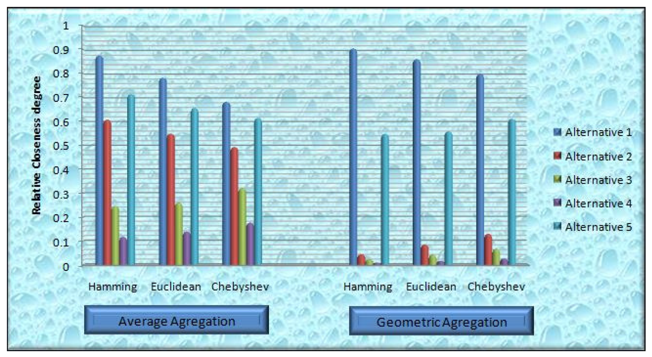
5.3. Sensitivity Analysis of Proposed LLDF-TOPSIS Method

In this part, we perform a sensitivity analysis for the proposed LLDF-TOPSIS method by concerning both the operators LLDFWAA and LLDFWGA. To execute this, we consider Example 14. The results are displayed in

Table 6. Sensitivity analysis of proposed LLDF-TOPSIS method by concerning LLDFWAA operator.

℘	Relative Closeness Degree					Ranking Order
1	0.8770978	0.6079344	0.2465916	0.1168285	0.7146982	${\hslash }_1\succ {\hslash }_5\succ {\hslash }_2\succ {\hslash }_3\succ {\hslash }_4$
10	0.692612	0.4979212	0.3049491	0.1747861	0.6209107	${\hslash }_1\succ {\hslash }_5\succ {\hslash }_2\succ {\hslash }_3\succ {\hslash }_4$
50	0.6830108	0.4934664	0.3216701	0.176642	0.6157014	${\hslash }_1\succ {\hslash }_5\succ {\hslash }_2\succ {\hslash }_3\succ {\hslash }_4$
100	0.6829103	0.493465	0.3218461	0.176642	0.6156959	${\hslash }_1\succ {\hslash }_5\succ {\hslash }_2\succ {\hslash }_3\succ {\hslash }_4$
500	0.6829091	0.493465	0.3218475	0.176642	0.6156959	${\hslash }_1\succ {\hslash }_5\succ {\hslash }_2\succ {\hslash }_3\succ {\hslash }_4$
550	0.6829091	0.493465	0.3218475	0	NaN	Inconsistent
1000	NaN	NaN	0	0	NaN	Inconsistent

In the table, NaN = not a number.

and

Table 7. Sensitivity analysis of proposed LLDF-TOPSIS method by concerning LLDFWGA operator.

℘	Relative Closeness Degree					Ranking Order
1	0.9067847	0.0455072	0.0219377	0.00833	0.5488545	${\hslash }_1\succ {\hslash }_5\succ {\hslash }_2\succ {\hslash }_3\succ {\hslash }_4$
10	0.8030421	0.1281813	0.0661199	0.0261452	0.5994666	${\hslash }_1\succ {\hslash }_5\succ {\hslash }_2\succ {\hslash }_3\succ {\hslash }_4$
50	0.7990682	0.1297514	0.0670557	0.0265668	0.6108875	${\hslash }_1\succ {\hslash }_5\succ {\hslash }_2\succ {\hslash }_3\succ {\hslash }_4$
100	0.7990677	0.1297514	0.0670557	0.0265668	0.6112875	${\hslash }_1\succ {\hslash }_5\succ {\hslash }_2\succ {\hslash }_3\succ {\hslash }_4$
500	0.7990677	0.1297514	0.0670557	0	0.6113077	${\hslash }_1\succ {\hslash }_5\succ {\hslash }_2\succ {\hslash }_3\succ {\hslash }_4$
550	0.7990677	0	0	0	0.6113077	Inconsistent
1000	NaN	0	0	0	NaN	Inconsistent

In the table, NaN = not a number.

. From Table 6 and Table 7, we observe that the proposed LLDF-TOPSIS method through both the operators LLDFWAA and LLDFWGA generates a consistent ranking order from $\wp =1$ to $\wp =500$. It starts to generate inconsistent ranking order from $\wp =500$ to $\wp =550$, and completely generates inconsistent ranking order at $\wp =1000$ and above.

5.4. Comparative Analysis to Show the Superiority of the Proposed LLDF-TOPSIS Method

In this section, we compare our proposed LLDF-TOPSIS method with some existing methods in

Table 8. Comparison of the proposed LLDF-TOPSIS method with existing methods.

Problem	Existing Methods	Ranking Order	Proposed LLDF-TOPSIS Method	Ranking Order
Combined Tables 10–12 ($LDFS$) (Riaz, & Hashmi, 2019)	Algorithm 2 ($SF,ESF$) (Riaz, & Hashmi, 2019)	$S_2\succ S_4\succ S_3\succ S_1$	$LLDFWAA$, $LLDFWGA$$(\wp =1)$	$S_2\succ S_4\succ S_3\succ S_1$
	Algorithm 2 ($QSF$) (Riaz, & Hashmi, 2019)	$S_4\succ S_2\succ S_3\succ S_1$	$LLDFWAA$, $LLDFWGA$$(\wp =2$, $\infty )$	$S_2\succ S_4\succ S_1\succ S_3$
Example 7.2, Table 10 ($Lq-ROFS$) (Lin et al., 2020)	$LqROFWA$ (Lin et al., 2020)	$A_1\succ A_2\succ A_4\succ A_3$	$LLDFWAA$, $LLDFWGA$$(\wp =1,2,\infty )$	$A_1\succ A_2\succ A_4\succ A_3$
Example 5.3, Table 5 ($LIFS$) (Garg, & Kumar, 2019)	LIFWG (Zhang, 2014), LIFWPA, LIFWPG (Liu, & Qin, 2017), LCNWG (Garg, 2018b), LIFWA (Chen et al., 2015), LIFEWA (Garg, & Kumar, 2018), ILIFWA (Liu, & Wang, 2017), LCNWPG (Garg, & Kumar, 2019)	${\nu }_2\succ {\nu }_3\succ {\nu }_4\succ {\nu }_5\succ {\nu }_1$	$LLDFWAA$, $LLDFWGA$$(\wp =1,2,\infty )$	${\nu }_2\succ {\nu }_3\succ {\nu }_4\succ {\nu }_5\succ {\nu }_1$
Illustrative Example ($LIFS$) (Zhang et al., 2017)	EOA (Zhang et al., 2017)	$a_4\succ a_1\succ a_3\succ a_2$	$LLDFWAA$$(\wp =1,2,\infty )$, $LLDFWGA$$(\wp =1,2)$	$a_4\succ a_1\succ a_3\succ a_2$
			$LLDFWGA$$(\wp =\infty )$	$a_4\succ a_3\succ a_1\succ a_2$
Example, Table 6 ($LIFS$) (Liu, & Wang, 2017)	ILIFWA (Liu, & Wang, 2017), ILIFWPA (Liu, & Wang, 2017), LIFWA (Chen et al., 2015), LIFWPA (Liu, & Qin, 2017)	$A_2\succ A_4\succ A_3\succ A_1$	$LLDFWAA$, $LLDFWGA$$(\wp =1,2,\infty )$	$A_2\succ A_4\succ A_1\succ A_3$
Example 5.5 ($LIFS$) (Garg, & Kumar, 2019)	$GAO$ (Liu, & Qin, 2017), $GAO$ (Chen et al., 2015)	${\nu }_1={\nu }_2$	$LLDFWAA$$(\wp =1,2,\infty )$	${\nu }_2\succ {\nu }_1$
			$LLDFWGA$$(\wp =1,2,\infty )$	${\nu }_1={\nu }_2$

to show the superiority of our proposed one. The LDFS can be generalized into the LLDFS. To utilize the proposed LLDF-TOPSIS method to solve the decision-making (DM) problems in LDF, the DM problem (combined Tables 10–12) in the article (Riaz & Hashmi, 2019) under the environment of LDFS can be solved by the proposed LLDF-TOPSIS method through the LLDFWAA operator and $LLDFWGA$ operator $(\wp =1)$. The ranking exactly matches the existing Algorithm 2 (score function (SF), expectation score function (ESF)) (Riaz & Hashmi, 2019) in the LDFS. However, there is a little variation in the ranking of the proposed LLDF-TOPSIS method through the LLDFWAA operators $(\wp =2,\infty )$ and LLDFWGA operators $(\wp =2,\infty )$ with the ranking of Algorithm 2 (quadratic score function (QSF)) (Riaz, & Hashmi, 2019) in LDFS. The linguistic q-rung orthopair fuzzy number (Lq-ROFN) as well as the linguistic intuitionistic fuzzy number (LIFN) of the form $\mathfrak{N}=\left(\langle {ł}_{\rho },{ł}_{\sigma }\rangle \right)$ can be viewed as an LLDFN, $\mathfrak{N}=(\langle 0,0\rangle ,\langle {ł}_{\rho },{ł}_{\sigma }\rangle )$. It enables us to compare the proposed LLDF-TOPSIS method with the existing methods in the Lq-ROFS and LIFS. The ranking of Example 7.2 (Table 10) (Lin et al., 2020) for the existing method Lq-ROFWA (Lin et al., 2020) in Lq-ROFS is the same as the ranking of the proposed LLDF-TOPSIS method through the operators of LLDFWAA and LLDFWGA $(\wp =1,2,\infty )$. The ranking of Example 5.3 (Table 5) (Garg, & Kumar, 2019) for the existing methods (LIFWG (Zhang, 2014), LIFWPA, LIFWPG (Liu, & Qin, 2017), LCNWG (Garg, 2018b), LIFWA (Chen et al., 2015), LIFEWA (Garg, & Kumar, 2018), ILIFWA (Liu, & Wang, 2017), LCNWPG (Garg, & Kumar, 2019)) in LIFS coincides with the proposed LLDF-TOPSIS method through the LLDFWAA operator and LLDFWGA operator $(\wp =1,2,\infty )$. The ranking of the proposed LLDF-TOPSIS method through the operators of LLDFWAA $(\wp =1,2,\infty )$ and LLDFWGA $(\wp =1,2)$ matches the existing method (extended outranking approach (EOA)) (Zhang et al., 2017) in LIFS for the illustrative example (Zhang et al., 2017), but through the LLDFWGA operator $(\wp =\infty )$, the result is a little deviated. The ranking of the proposed LLDF-TOPSIS method through the LLDFWAA and LLDFWGA operators $(\wp =1,2,\infty )$ deviates little from the ranking of methods ILIFWA (Liu, & Wang, 2017), ILIFWPA (Liu, & Wang, 2017), LIFWA (Chen et al., 2015), and LIFWPA (Liu, & Qin, 2017) for example (Table 6) (Liu, & Wang, 2017) in LIFS. The existing methods in the papers (Liu, & Qin, 2017) and (Chen et al., 2015) and the proposed LLDF-TOPSIS method through the LLDFWGA operator $(\wp =1,2,\infty )$ for Example 5.5 (Garg, & Kumar, 2019) in LIFS fail to produce the ranking, but the proposed LLDF-TOPSIS method through the LLDFWAA operator $(\wp =1,2,\infty )$ produces the feasible ranking. From the overall comparison, we conclude that our proposed LLDF-TOPSIS method through the LLDFWAA operator $(\wp =1,2,\infty )$ is more convenient than, and superior to, the other methods.

5.5. Validity of Proposed LLDF-TOPSIS Method

In 2008, Wang and Triantaphyllou (2008) introduced some test criteria to check the validity of a decision-making (DM) method, as shown in

Table 9. Wang–Triantaphyllou’s test criteria to check the validity of decision-making method.

Test Criteria	Description
1	The best alternative should not be changed if any nonoptimal alternative is worsening further without
	interchanging the position of decision-making criteria.
2	Transitive properties should be satisfied by the DM method.
3	If a DM problem is decomposed further, the combined ranking order of the decomposed DM problem
	should be matching with the original DM problem.

. In this section, we verify Wang–Triantaphyllou’s test criteria by employing Example 14 to show the validity of our proposed LLDF-TOPSIS method.

5.5.1. Validity of Proposed LLDF-TOPSIS Method by Test Criterion

The nonoptimal alternatives ${\hslash }_2,{\hslash }_3,{\hslash }_4$, and ${\hslash }_5$ in the decision matrix $\Lambda$ of Example 14 are further worsening arbitrarily into ${\hslash }_2^{{}^{\prime }},{\hslash }_3^{{}^{\prime }},{\hslash }_4^{{}^{\prime }}$, and ${\hslash }_5^{{}^{\prime }}$, respectively, without interchanging the position of decision criteria, as follows.

$${\hslash }_2^{{}^{\prime }}=\left(\begin{array}{ccccccc}& (\langle {ł}_1,{ł}_4\rangle ,\langle {ł}_0,{ł}_4\rangle )& (\langle {ł}_1,{ł}_4\rangle ,\langle {ł}_2,{ł}_2\rangle )& (\langle {ł}_1,{ł}_4\rangle ,\langle {ł}_1,{ł}_3\rangle )& (\langle {ł}_1,{ł}_3\rangle ,\langle {ł}_0,{ł}_4\rangle )& (\langle {ł}_1,{ł}_3\rangle ,\langle {ł}_0,{ł}_4\rangle )& (\langle {ł}_1,{ł}_3\rangle ,\langle {ł}_0,{ł}_4\rangle )\end{array}\right)$$

$${\hslash }_3^{{}^{\prime }}=\left(\begin{array}{ccccccc}& (\langle {ł}_1,{ł}_4\rangle ,\langle {ł}_1,{ł}_3\rangle )& (\langle {ł}_0,{ł}_3\rangle ,\langle {ł}_1,{ł}_3\rangle )& (\langle {ł}_2,{ł}_3\rangle ,\langle {ł}_1,{ł}_3\rangle )& (\langle {ł}_1,{ł}_4\rangle ,\langle {ł}_1,{ł}_3\rangle )& (\langle {ł}_1,{ł}_4\rangle ,\langle {ł}_0,{ł}_3\rangle )& (\langle {ł}_1,{ł}_3\rangle ,\langle {ł}_0,{ł}_4\rangle )\end{array}\right)$$

$${\hslash }_4^{{}^{\prime }}=\left(\begin{array}{ccccccc}& (\langle {ł}_1,{ł}_4\rangle ,\langle {ł}_0,{ł}_4\rangle )& (\langle {ł}_0,{ł}_4\rangle ,\langle {ł}_1,{ł}_3\rangle )& (\langle {ł}_1,{ł}_4\rangle ,\langle {ł}_0,{ł}_3\rangle )& (\langle {ł}_0,{ł}_4\rangle ,\langle {ł}_1,{ł}_3\rangle )& (\langle {ł}_2,{ł}_4\rangle ,\langle {ł}_1,{ł}_3\rangle )& (\langle {ł}_1,{ł}_4\rangle ,\langle {ł}_1,{ł}_3\rangle )\end{array}\right)$$

$${\hslash }_5^{{}^{\prime }}=\left(\begin{array}{ccccccc}& (\langle {ł}_0,{ł}_4\rangle ,\langle {ł}_1,{ł}_3\rangle )& (\langle {ł}_2,{ł}_4\rangle ,\langle {ł}_1,{ł}_3\rangle )& (\langle {ł}_1,{ł}_3\rangle ,\langle {ł}_0,{ł}_4\rangle )& (\langle {ł}_1,{ł}_4\rangle ,\langle {ł}_1,{ł}_3\rangle )& (\langle {ł}_2,{ł}_3\rangle ,\langle {ł}_1,{ł}_3\rangle )& (\langle {ł}_0,{ł}_3\rangle ,\langle {ł}_1,{ł}_3\rangle )\end{array}\right)$$

For instance, the alternative ${\hslash }_2$ in the decision matrix $\Lambda$ of Example 14 is replaced by the worsened alternative ${\hslash }_2^{{}^{\prime }}$, then the original decision matrix $\Lambda$ of Example 14 becomes a modified decision matrix ${\Lambda }_1^{{}^{\prime }}$, as follows.

$${\Lambda }_1^{{}^{\prime }}=\left[\begin{array}{ccccccc}{\hslash }_1& (\langle {ł}_4,{ł}_1\rangle ,\langle {ł}_4,{ł}_0\rangle )& (\langle {ł}_3,{ł}_2\rangle ,\langle {ł}_3,{ł}_0\rangle )& (\langle {ł}_4,{ł}_2\rangle ,\langle {ł}_3,{ł}_1\rangle )& (\langle {ł}_4,{ł}_3\rangle ,\langle {ł}_3,{ł}_1\rangle )& (\langle {ł}_4,{ł}_1\rangle ,\langle {ł}_2,{ł}_0\rangle )& (\langle {ł}_4,{ł}_1\rangle ,\langle {ł}_3,{ł}_0\rangle )\\ {\hslash }_2^{{}^{\prime }}& (\langle {ł}_1,{ł}_4\rangle ,\langle {ł}_0,{ł}_4\rangle )& (\langle {ł}_1,{ł}_4\rangle ,\langle {ł}_2,{ł}_2\rangle )& (\langle {ł}_1,{ł}_4\rangle ,\langle {ł}_1,{ł}_3\rangle )& (\langle {ł}_1,{ł}_3\rangle ,\langle {ł}_0,{ł}_4\rangle )& (\langle {ł}_1,{ł}_3\rangle ,\langle {ł}_0,{ł}_4\rangle )& (\langle {ł}_1,{ł}_3\rangle ,\langle {ł}_0,{ł}_4\rangle )\\ {\hslash }_3& (\langle {ł}_2,{ł}_4\rangle ,\langle {ł}_2,{ł}_2\rangle )& (\langle {ł}_2,{ł}_4\rangle ,\langle {ł}_3,{ł}_1\rangle )& (\langle {ł}_2,{ł}_3\rangle ,\langle {ł}_1,{ł}_3\rangle )& (\langle {ł}_1,{ł}_2\rangle ,\langle {ł}_1,{ł}_3\rangle )& (\langle {ł}_1,{ł}_2\rangle ,\langle {ł}_0,{ł}_2\rangle )& (\langle {ł}_1,{ł}_2\rangle ,\langle {ł}_0,{ł}_4\rangle )\\ {\hslash }_4& (\langle {ł}_1,{ł}_3\rangle ,\langle {ł}_0,{ł}_4\rangle )& (\langle {ł}_2,{ł}_4\rangle ,\langle {ł}_1,{ł}_3\rangle )& (\langle {ł}_1,{ł}_4\rangle ,\langle {ł}_2,{ł}_2\rangle )& (\langle {ł}_1,{ł}_4\rangle ,\langle {ł}_1,{ł}_3\rangle )& (\langle {ł}_2,{ł}_3\rangle ,\langle {ł}_1,{ł}_3\rangle )& (\langle {ł}_1,{ł}_4\rangle ,\langle {ł}_1,{ł}_3\rangle )\\ {\hslash }_5& (\langle {ł}_2,{ł}_2\rangle ,\langle {ł}_1,{ł}_3\rangle )& (\langle {ł}_3,{ł}_0\rangle ,\langle {ł}_3,{ł}_1\rangle )& (\langle {ł}_2,{ł}_3\rangle ,\langle {ł}_2,{ł}_2\rangle )& (\langle {ł}_3,{ł}_1\rangle ,\langle {ł}_1,{ł}_0\rangle )& (\langle {ł}_3,{ł}_3\rangle ,\langle {ł}_1,{ł}_2\rangle )& (\langle {ł}_1,{ł}_3\rangle ,\langle {ł}_1,{ł}_0\rangle )\end{array}\right]$$

If the proposed LLDF-TOPSIS method concerning the LLDFWAA operator, Hamming ($\wp =1$), Euclidean ($\wp =2$), and Chebyshev ($\wp =\infty$) distances is utilized for the modified decision matrix ${\Lambda }_1^{{}^{\prime }}$ of Example 14, we obtain the relative closeness degree and the modified ranking order as per Table 10.

Table 10. Ranking of LLDF-TOPSIS by concerning LLDFWAA operator for modified ${\Lambda }_1^{{}^{\prime }}$ of Example 14.

℘	Relative Closeness Degree					Modified Ranking Order
1	0.8806164	0.0562014	0.2681607	0.1421125	0.722866	${\hslash }_1\succ {\hslash }_5\succ {\hslash }_3\succ {\hslash }_4\succ {\hslash }_2^{{}^{\prime }}$
2	0.7897406	0.0710804	0.2777813	0.1615761	0.6650673	${\hslash }_1\succ {\hslash }_5\succ {\hslash }_3\succ {\hslash }_4\succ {\hslash }_2^{{}^{\prime }}$
∞	0.6829091	0.1148618	0.3218475	0.176642	0.6156959	${\hslash }_1\succ {\hslash }_5\succ {\hslash }_3\succ {\hslash }_4\succ {\hslash }_2^{{}^{\prime }}$

Table 10. Ranking of LLDF-TOPSIS by concerning LLDFWAA operator for modified ${\Lambda }_1^{{}^{\prime }}$ of Example 14.

℘	Relative Closeness Degree					Modified Ranking Order
1	0.8806164	0.0562014	0.2681607	0.1421125	0.722866	${\hslash }_1\succ {\hslash }_5\succ {\hslash }_3\succ {\hslash }_4\succ {\hslash }_2^{{}^{\prime }}$
2	0.7897406	0.0710804	0.2777813	0.1615761	0.6650673	${\hslash }_1\succ {\hslash }_5\succ {\hslash }_3\succ {\hslash }_4\succ {\hslash }_2^{{}^{\prime }}$
∞	0.6829091	0.1148618	0.3218475	0.176642	0.6156959	${\hslash }_1\succ {\hslash }_5\succ {\hslash }_3\succ {\hslash }_4\succ {\hslash }_2^{{}^{\prime }}$

If the proposed LLDF-TOPSIS method by concerning the LLDFWGA operator, Hamming ($\wp =1$), Euclidean ($\wp =2$), and Chebyshev ($\wp =\infty$) distances for the modified decision matrix ${\Lambda }^{{}^{\prime }}$ of Example 14 is utilized, we obtain the relative closeness degree and the modified ranking order as per

Table 11. Ranking of LLDF-TOPSIS by concerning LLDFWGA operator for modified ${\Lambda }_1^{{}^{\prime }}$ of Example 14.

℘	Relative Closeness Degree					Modified Ranking Order
1	0.9074373	0	0.0287855	0.015273	0.5520131	${\hslash }_1\succ {\hslash }_5\succ {\hslash }_3\succ {\hslash }_4\succ {\hslash }_2^{{}^{\prime }}$
2	0.8619556	0	0.0553555	0.0298173	0.5608168	${\hslash }_1\succ {\hslash }_5\succ {\hslash }_3\succ {\hslash }_4\succ {\hslash }_2^{{}^{\prime }}$
∞	0.7990677	0	0.0867378	0.0479747	0.6113077	${\hslash }_1\succ {\hslash }_5\succ {\hslash }_3\succ {\hslash }_4\succ {\hslash }_2^{{}^{\prime }}$

.

From Table 10 and Table 11, we observe that the modified ranking order of LLDF-TOPSIS method concerning both LLDFWAA and LLDFWGA operators, Hamming, Euclidean, and Chebyshev distances for modified ${\Lambda }_1^{{}^{\prime }}$ of Example 14 is the same as ${\hslash }_1\succ {\hslash }_5\succ {\hslash }_3\succ {\hslash }_4\succ {\hslash }_2^{{}^{\prime }}$. This leads to deciding that ${\hslash }_1$ is the best alternative. It coincides with the best alternative of original decision matrix $\Lambda$ for Example 14. In the same way, other nonoptimal alternatives ${\hslash }_3,{\hslash }_4$, and ${\hslash }_5$ of decision matrix $\Lambda$ for Example 14 are further worsening into ${\hslash }_3^{{}^{\prime }},{\hslash }_4^{{}^{\prime }}$, and ${\hslash }_5^{{}^{\prime }}$, respectively, without interchanging the decision criteria. We obtain the modified decision matrices ${\Lambda }_3^{{}^{\prime }},{\Lambda }_4^{{}^{\prime }}$, and ${\Lambda }_5^{{}^{\prime }}$, respectively, for Example 14. If the proposed LLDF-TOPSIS method by concerning both LLDFWAA and LLDFWGA operators, Hamming, Euclidean, and Chebyshev distances is utilized for modified decision matrix ${\Lambda }_i^{{}^{\prime }}$$(i=3,4,5)$ of Example 14, we obtain the modified ranking order as placed in

Table 12. Ranking of LLDF-TOPSIS by concerning the different worsened alternatives of Example 14.

Operator	Worsened	℘	Relative Closeness Degree					Modified
	Alternative							Ranking Order
		1	0.8805384	0.6189101	0.0981113	0.1415523	0.722685	${\hslash }_1\succ {\hslash }_5\succ {\hslash }_2\succ {\hslash }_4\succ {\hslash }_3^{{}^{\prime }}$
	${\hslash }_3^{{}^{\prime }}$	2	0.7886395	0.5602136	0.1035499	0.1498834	0.6638354	${\hslash }_1\succ {\hslash }_5\succ {\hslash }_2\succ {\hslash }_4\succ {\hslash }_3^{{}^{\prime }}$
		∞	0.6829091	0.493465	0.1364624	0.176642	0.6245059	${\hslash }_1\succ {\hslash }_5\succ {\hslash }_2\succ {\hslash }_4\succ {\hslash }_3^{{}^{\prime }}$
		1	0.8844572	0.6314113	0.2917056	0.070326	0.731782	${\hslash }_1\succ {\hslash }_5\succ {\hslash }_2\succ {\hslash }_3\succ {\hslash }_4^{{}^{\prime }}$
$LLDFWAA$	${\hslash }_4^{{}^{\prime }}$	2	0.7953105	0.5681692	0.2971628	0.0884888	0.6689092	${\hslash }_1\succ {\hslash }_5\succ {\hslash }_2\succ {\hslash }_3\succ {\hslash }_4^{{}^{\prime }}$
		∞	0.6964529	0.493465	0.3455232	0.1256798	0.6245059	${\hslash }_1\succ {\hslash }_5\succ {\hslash }_2\succ {\hslash }_3\succ {\hslash }_4^{{}^{\prime }}$
		1	0.9607239	0.6818531	0.3074783	0.1730353	0.1228976	${\hslash }_1\succ {\hslash }_2\succ {\hslash }_3\succ {\hslash }_4\succ {\hslash }_5^{{}^{\prime }}$
	${\hslash }_5^{{}^{\prime }}$	2	0.9258151	0.5919224	0.3090222	0.1976132	0.1319819	${\hslash }_1\succ {\hslash }_2\succ {\hslash }_3\succ {\hslash }_4\succ {\hslash }_5^{{}^{\prime }}$
		∞	0.8814951	0.5092861	0.3218475	0.2691846	0.1729335	${\hslash }_1\succ {\hslash }_2\succ {\hslash }_3\succ {\hslash }_4\succ {\hslash }_5^{{}^{\prime }}$
		1	0.914351	0.1229836	0	0.0888241	0.5854741	${\hslash }_1\succ {\hslash }_5\succ {\hslash }_2\succ {\hslash }_4\succ {\hslash }_3^{{}^{\prime }}$
	${\hslash }_3^{{}^{\prime }}$	2	0.8726924	0.2161282	0	0.1618951	0.5890372	${\hslash }_1\succ {\hslash }_5\succ {\hslash }_2\succ {\hslash }_4\succ {\hslash }_3^{{}^{\prime }}$
		∞	0.8151825	0.3048466	0	0.2405407	0.6113077	${\hslash }_1\succ {\hslash }_5\succ {\hslash }_2\succ {\hslash }_4\succ {\hslash }_3^{{}^{\prime }}$
		1	0.914351	0.1229836	0.1013273	0	0.5854741	${\hslash }_1\succ {\hslash }_5\succ {\hslash }_2\succ {\hslash }_3\succ {\hslash }_4^{{}^{\prime }}$
$LLDFWGA$	${\hslash }_4^{{}^{\prime }}$	2	0.8726924	0.2161282	0.1822886	0	0.5890372	${\hslash }_1\succ {\hslash }_5\succ {\hslash }_2\succ {\hslash }_3\succ {\hslash }_4^{{}^{\prime }}$
		∞	0.8151825	0.3048466	0.2654133	0	0.6113077	${\hslash }_1\succ {\hslash }_5\succ {\hslash }_2\succ {\hslash }_3\succ {\hslash }_4^{{}^{\prime }}$
		1	0.9401197	0.1264496	0.1041829	0.0913274	0	${\hslash }_1\succ {\hslash }_2\succ {\hslash }_3\succ {\hslash }_4\succ {\hslash }_5^{{}^{\prime }}$
	${\hslash }_5^{{}^{\prime }}$	2	0.8896411	0.2223404	0.1875491	0.1665722	0	${\hslash }_1\succ {\hslash }_2\succ {\hslash }_3\succ {\hslash }_4\succ {\hslash }_5^{{}^{\prime }}$
		∞	0.8321007	0.3209245	0.2802499	0.2544685	0	${\hslash }_1\succ {\hslash }_2\succ {\hslash }_3\succ {\hslash }_4\succ {\hslash }_5^{{}^{\prime }}$

. From Table 12, we observe that ${\hslash }_1$ is the best alternative for all modified decision matrices ${\Lambda }_3^{{}^{\prime }},{\Lambda }_4^{{}^{\prime }}$, and ${\Lambda }_5^{{}^{\prime }}$ by utilizing the proposed LLDF-TOPSIS method by concerning both LLDFWAA and LLDFWGA operators, Hamming, Euclidean, and Chebyshev distances. It coincides with the original decision matrix $\Lambda$ for Example 14. Therefore, the proposed LLDF-TOPSIS method is valid according to test criterion 1.

5.5.2. Validity of Proposed LLDF-TOPSIS Method by Test Criteria 2 and 3

The decision matrix $\Lambda$ of Example 14 is further decomposed into sub-decision matrices ${\Lambda }_i$$(i=1\cdots 5)$. The set of alternatives for sub-decision matrices ${\Lambda }_i$$(i=1\cdots 5)$ are $\{{\hslash }_1,{\hslash }_2\}$, $\{{\hslash }_1,{\hslash }_3\}$, $\{{\hslash }_2,{\hslash }_3\}$, $\{{\hslash }_1,{\hslash }_2,{\hslash }_3\}$, $\{{\hslash }_1,{\hslash }_2,{\hslash }_5\}$, and $\{{\hslash }_2,{\hslash }_3,{\hslash }_4,{\hslash }_5\}$ respectively. The ranking of alternatives for decomposed sub-decision matrices ${\Lambda }_i$$(i=1\cdots 5)$ by concerning the proposed LLDF-TOPSIS method is displayed in

Table 13. Ranking of LLDF-TOPSIS for decomposed sub-decision matrices ${\Lambda }_i$$(i=1\dots 5)$ in Example 14.

Operator	Alternatives of Sub Decision Matrix	℘	Relative Closeness Degree				Decomposed Ranking Order
$LLDFWAA$		1	0.8974024	0.1689318			${\hslash }_1\succ {\hslash }_2$
	$\{{\hslash }_1,{\hslash }_2\}$	2	0.8745796	0.1947799			${\hslash }_1\succ {\hslash }_2$
		∞	0.8692927	0.1984454			${\hslash }_1\succ {\hslash }_2$
		1	0.9814656	0.0311427			${\hslash }_1\succ {\hslash }_3$
	$\{{\hslash }_1,{\hslash }_3\}$	2	0.964944	0.0578486			${\hslash }_1\succ {\hslash }_3$
		∞	0.942311	0.0932726			${\hslash }_1\succ {\hslash }_3$
		1	0.8734156	0.2065581			${\hslash }_2\succ {\hslash }_3$
	$\{{\hslash }_2,{\hslash }_3\}$	2	0.8439595	0.189799			${\hslash }_2\succ {\hslash }_3$
		∞	0.7966899	0.218296			${\hslash }_2\succ {\hslash }_3$
		1	0.9528451	0.6180329	0.1685587		${\hslash }_1\succ {\hslash }_2\succ {\hslash }_3$
	$\{{\hslash }_1,{\hslash }_2,{\hslash }_3\}$	2	0.9126114	0.5370542	0.1803958		${\hslash }_1\succ {\hslash }_2\succ {\hslash }_3$
		∞	0.8692927	0.4434209	0.2033101		${\hslash }_1\succ {\hslash }_2\succ {\hslash }_3$
		1	0.8543184	0.5352665	0.6618184		${\hslash }_1\succ {\hslash }_5\succ {\hslash }_2$
	$\{{\hslash }_1,{\hslash }_2,{\hslash }_5\}$	2	0.7548802	0.4902375	0.5959521		${\hslash }_1\succ {\hslash }_5\succ {\hslash }_2$
		∞	0.6722805	0.4296873	0.5486267		${\hslash }_1\succ {\hslash }_5\succ {\hslash }_2$
		1	0.7311555	0.2965727	0.1405082	0.859559	${\hslash }_5\succ {\hslash }_2\succ {\hslash }_3\succ {\hslash }_4$
	$\{{\hslash }_2,{\hslash }_3,{\hslash }_4,{\hslash }_5\}$	2	0.6834884	0.2929871	0.1534108	0.7827239	${\hslash }_5\succ {\hslash }_2\succ {\hslash }_3\succ {\hslash }_4$
		∞	0.6370337	0.3390346	0.176642	0.7191652	${\hslash }_5\succ {\hslash }_2\succ {\hslash }_3\succ {\hslash }_4$
$LLDFWGA$		1	0.9314519	0			${\hslash }_1\succ {\hslash }_2$
	$\{{\hslash }_1,{\hslash }_2\}$	2	0.8744534	0			${\hslash }_1\succ {\hslash }_2$
		∞	0.8171302	0			${\hslash }_1\succ {\hslash }_2$
		1	0.9655902	0			${\hslash }_1\succ {\hslash }_3$
	$\{{\hslash }_1,{\hslash }_3\}$	2	0.9347356	0			${\hslash }_1\succ {\hslash }_3$
		∞	0.8998191	0			${\hslash }_1\succ {\hslash }_3$
		1	0.1748091	0.0696136			${\hslash }_2\succ {\hslash }_3$
	$\{{\hslash }_2,{\hslash }_3\}$	2	0.192474	0.084444			${\hslash }_2\succ {\hslash }_3$
		∞	0.1938899	0.087411			${\hslash }_2\succ {\hslash }_3$
		1	0.9342374	0.0406366	0.0161826		${\hslash }_1\succ {\hslash }_2\succ {\hslash }_3$
	$\{{\hslash }_1,{\hslash }_2,{\hslash }_3\}$	2	0.8786336	0.0772039	0.031617		${\hslash }_1\succ {\hslash }_2\succ {\hslash }_3$
		∞	0.8171302	0.1214889	0.0521961		${\hslash }_1\succ {\hslash }_2\succ {\hslash }_3$
		1	0.9053393	0.0307077	0.5418594		${\hslash }_1\succ {\hslash }_5\succ {\hslash }_2$
	$\{{\hslash }_1,{\hslash }_2,{\hslash }_5\}$	2	0.8591502	0.0586376	0.5552184		${\hslash }_1\succ {\hslash }_5\succ {\hslash }_2$
		∞	0.7990677	0.090142	0.6113077		${\hslash }_1\succ {\hslash }_5\succ {\hslash }_2$
		1	0.0685769	0.033059	0.0125528	0.8270932	${\hslash }_5\succ {\hslash }_2\succ {\hslash }_3\succ {\hslash }_4$
	$\{{\hslash }_2,{\hslash }_3,{\hslash }_4,{\hslash }_5\}$	2	0.121811	0.0613379	0.02386	0.8158337	${\hslash }_5\succ {\hslash }_2\succ {\hslash }_3\succ {\hslash }_4$
		∞	0.1604973	0.0843859	0.033812	0.8053293	${\hslash }_5\succ {\hslash }_2\succ {\hslash }_3\succ {\hslash }_4$

. From Table 13, we observe that the decomposed ranking order for the decomposed sub-decision matrices ${\Lambda }_i$$(i=1\cdots 5)$ is ${\hslash }_1\succ {\hslash }_2$, ${\hslash }_1\succ {\hslash }_3$, ${\hslash }_2\succ {\hslash }_3$, ${\hslash }_1\succ {\hslash }_2\succ {\hslash }_3$, ${\hslash }_1\succ {\hslash }_5\succ {\hslash }_2$, and ${\hslash }_5\succ {\hslash }_2\succ {\hslash }_3\succ {\hslash }_4$, respectively, by concerning the proposed LLDF-TOPSIS method through the operators LLDFWAA, LLDFWGA, and distance measures Hamming ($\wp =1$), Euclidean ($\wp =2$), and Chebyshev ($\wp =\infty$). Hence, the combined ranking order is ${\hslash }_1\succ {\hslash }_5\succ {\hslash }_2\succ {\hslash }_3\succ {\hslash }_4$. It coincides with the original ranking order of the original decision matrix $\Lambda$ of Example 14. Moreover, transitivity property is held for the decomposed ranking order of decomposed sub-decision matrices ${\Lambda }_i$$(i=1\cdots 5)$. Therefore, the proposed LLDF-TOPSIS method is valid according to test criteria 2 and 3.

5.6. Advantages of the Proposed LLDF-TOPSIS Method

• While the concepts of LIFS, LPyFS, and Lq-ROFS can classify objects by linguistic degrees of membership and nonmembership, they cannot allow these objects to be handled with reference/control parameters represented by linguistic variables. The idea of LLDFS proposed in this paper fills this research gap. It centralizes linguistic reference/control parameters in the process of evaluating objects and thus extends existing concepts of LIFS, LPyFS, and Lq-ROFS. On the other hand, the LDFSs have a few obstacles to explicit qualitative arguments on degrees of membership, nonmembership, and reference/control parameters with real numbers. The LLDFSs give a different perspective to existing LDFSs by expressing LDF information based on linguistic variables. This leads to a wider application area of LDFSs (IFSs, PyFSs, q-ROFSs) in practice. Considering all these, it can be said that there is a close relationship between the proposed LLDFSs and multicriteria decision-making problems. The linguistic membership and nonmembership grades, as well as linguistic grades of reference parameters, play an important role in the proposed LLDF-TOPSIS method.
• The LLDF-TOPSIS approach is bendy, and without difficulty may be used for exceptional conditions of inputs and outputs. This technique is more bendy than others due to reference parameters and relaxation on degrees with real numbers. It will increase the space of grades and may be variedin step with the exceptional conditions in multicriteria decision-making methods. Consequently, the present techniques on the present notions of LIFSs, LPyFSs, Lq-ROFSs, and LDFSs come to be the unique case of our proposed LLDF-TOPSIS method. In other words, our proposed LLDF-TOPSIS approach is more well known than different current techniques. That is, it improves many decision-making methods based on the LIFS, LPyFS, Lq-ROFS, and LDFS (IFS, PyFS, q-ROFS).

5.7. Disadvantages of the Proposed LLDF-TOPSIS Method

• From Table 6 and Table 7, we recognize that our proposed LLDF-TOPSIS method fails for the big parameter ℘$(\wp \ge 550)$. However, the use of big parameters ℘ is rare. Thus, we can forget about it.
• Our proposed LLDF-TOPSIS approach cannot be carried out for the fuzzy multicriteria decision-making problems concerning impartial membership degrees, bipolarity, and hesitant types.

6. Conclusions

The proposed model and LMCDM issues are shown to be closely related. This link leads to the construction of a modified TOPSIS algorithm to handle uncertainty in multi-attribute data in a parametric way. LMCDM issues are satisfactorily solved by the linguistic linear Diophantine fuzzy TOPSIS (LLDF-TOPSIS) approach, which enhances the TOPSIS methods based on LIFSs, LPyFSs, and Lq-ROFSs. The parameters and special situations of Minkowski-type distances between two LLDFSs were also examined. In the work inspired by LLDFNs, LLDFSs expressed ambiguous evaluation information on linguistic terms specified in linguistic multicriteria decision-making. The LLDF-TOPSIS method was proposed and contrasted with well-known linguistic fuzzy TOPSIS methods for linguistic multicriteria decision-making situations.

The key contributions can be summarized in the following.

(1) 

The emergence of LLDFSs allows dealing with some special cases where the data collected in LDFS-based evaluations are linguistic terms rather than crisp numbers in the interval [0,1].

(2) 

Some linguistic linear Diophantine fuzzy aggregation operators discussed in this study conduct the improvement of LLDFSs in both theoretical and practical aspects.

(3) 

The proposed distance measures of LLDFSs allow coping with many issues such as medical diagnosis, clustering analysis, and pattern recognition in different fields.

(4) 

The developed LLDF-TOPSIS method enriches fuzzy decision-making theory and provides a new method for decision-makers in the surrounding of LLDFSs (and also LFSs, LIFSs, LPyFSs, and Lq-ROFSs).

In future research, we will investigate the contributions of the proposed aggregation operators and distance measures for problems in other domains, such as multiobjective programming, clustering, uncertain system, and supplier selection. Our efforts will aim to fill this research gap.

References

1. Zadeh, L.A. Fuzzy sets. Inf. Control 1965, 8, 338–353. [Google Scholar] [CrossRef] [Green Version]
2. Cateni, S.; Colla, V.; Nastasi, G. A multivariate fuzzy system applied for outliers detection. J. Intell. Fuzzy Syst. 2013, 24, 889–903. [Google Scholar] [CrossRef]
3. Das, S.; Guha, D.; Dutta, B. Medical diagnosis with the aid of using fuzzy logic and intuitionistic fuzzy logic. Appl. Intell. 2016, 45, 850–867. [Google Scholar] [CrossRef]
4. Yager, R.R. Multiple objective decision-making using fuzzy sets. Int. J. -Man-Mach. Stud. 1977, 9, 375–382. [Google Scholar] [CrossRef]
5. Atanassov, K.T. Intuitionistic fuzzy sets. Fuzzy Sets Syst. 1986, 20, 87–96. [Google Scholar] [CrossRef]
6. Yager, R.R. Pythagorean fuzzy subsets. In Proceedings of the IFSA World Congress and NAFIPS Annual Meeting, Edmonton, AB, Canada, 24–28 June 2013; pp. 57–61. [Google Scholar]
7. Yager, R.R. Generalized orthopair fuzzy sets. IEEE Trans. Fuzzy Syst. 2017, 25, 1222–1230. [Google Scholar] [CrossRef]
8. Peng, X.; Luo, Z. A review of q-rung orthopair fuzzy information: Bibliometrics and future directions. Artif. Intell. Rev. 2021, 54, 3361–3430. [Google Scholar] [CrossRef]
9. Rahman, K.; Abdullah, S.; Khan, M.S.A.; Ibrar, M.; Husain, F. Some basic operations on Pythagorean fuzzy sets. J. Appl. Environ. Biol. Sci. 2017, 7, 111–119. [Google Scholar]
10. Ejegwa, P.A. New similarity measures for Pythagorean fuzzy sets with applications. Int. J. Fuzzy Comput. Model. 2020, 3, 75–94. [Google Scholar] [CrossRef]
11. Farhadinia, B.; Effati, S.; Chiclana, F. A family of similarity measures for q-rung orthopair fuzzy sets and their applications to multiple criteria decision-making. Int. J. Intell. Syst. 2021, 36, 1535–1559. [Google Scholar] [CrossRef]
12. Garg, H. An improved cosine similarity measure for intuitionistic fuzzy sets and their applications to decision-making process. Hacet. J. Math. Stat. 2018, 47, 1578–1594. [Google Scholar] [CrossRef]
13. Hussian, Z.; Yang, M.-S. Distance and similarity measures of Pythagorean fuzzy sets based on the Hausdorff metric with application to fuzzy TOPSIS. Int. J. Intell. Syst. 2019, 34, 2633–2654. [Google Scholar] [CrossRef]
14. Aydemir, S.B.; Gunduz, S.Y. A novel approach to multi-attribute group decision-making based on power neutrality aggregation operator for q-rung orthopair fuzzy sets. Int. J. Intell. Syst. 2019, 36, 1454–1481. [Google Scholar] [CrossRef]
15. Biswas, A.; Deb, N. Pythagorean fuzzy Schweizer and Sklar power aggregation operators for solving multi-attribute decision-making problems. Garnular Comput. 2021, 6, 991–1007. [Google Scholar] [CrossRef]
16. Jana, C.; Senepati, T.; Pal, M. Pythagorean fuzzy Dombi aggregation operators and its applications in multiple attribute decision-making. Int. J. Intell. Syst. 2019, 34, 2019–2038. [Google Scholar] [CrossRef]
17. Akram, M.; Amjad, U.; Alcantud, J.C.R.; Santos-García, G. Complex fermatean fuzzy N-soft sets: A new hybrid model with applications. J. Ambient. Intell. Humaniz. Comput. 2022. [Google Scholar] [CrossRef] [PubMed]
18. Feng, F.; Zheng, Y.; Sun, B.; Akram, M. Novel score functions of generalized orthopair fuzzy membership grades with application to multiple attribute decision-making. Granul. Comput. 2022, 7, 95–111. [Google Scholar] [CrossRef]
19. Karaaslan, F.; Çağman, N. Parameter trees based on soft set theory and their similarity measures. Soft Comput. 2022, 26, 4629–4639. [Google Scholar] [CrossRef]
20. Riaz, M.; Hashmi, M.R. Linear Diophantine fuzzy set and its applications towards multi-attribute decision-making problems. J. Intell. Fuzzy Syst. 2019, 37, 5417–5439. [Google Scholar] [CrossRef]
21. Ayub, S.; Shabir, M.; Riaz, M.; Aslam, M.; Chinram, R. Linear Diophantine fuzzy relations and their algebraic properties with decision-making. Symmetry 2021, 13, 945. [Google Scholar] [CrossRef]
22. Kamacı, H. Complex linear Diophantine fuzzy sets and their cosine similarity measures with applications. Complex Intell. Syst. 2021. [Google Scholar] [CrossRef]
23. Kamacı, H. Linear Diophantine fuzzy algebraic structures. J. Ambient. Intell. Humaniz. Comput. 2021, 12, 10353–10373. [Google Scholar] [CrossRef]
24. Almagrabi, A.O.; Abdullah, S.; Shams, M.; Al-Otaibi, Y.D.; Ashraf, S. A new approach to q-linear Diophantine fuzzy emergency decision support system for COVID19. J. Ambient. Intell. Humaniz. Comput. 2022, 13, 1687–1713. [Google Scholar] [CrossRef] [PubMed]
25. Mahmood, T.; Ali, Z.; Aslam, M.; Chinram, R. Generalized Hamacher aggregation operators based on linear Diophantine uncertain linguistic setting and their applications in decision-making problems. IEEE Access 2021, 9, 126748–126764. [Google Scholar]
26. Mahmood, T.; Ali, Z.; Ullah, K.; Khan, Q.; Alsanad, A.; Mosleh, M.A.A. Linear Diophantine uncertain linguistic power Einstein aggregation operators and their applications to multiattribute decision-making. Complexity 2021, 2021, 25. [Google Scholar] [CrossRef]
27. Ashraf, S.; Abdullah, S.; Mahmood, T.; Ghani, F.; Mahmood, T. Spherical fuzzy sets and their applications in multi-attribute decision-making problems. J. Intell. Fuzzy Syst. 2019, 36, 2829–2844. [Google Scholar] [CrossRef]
28. Cuong, B.C. Picture fuzzy sets. J. Comput. Sci. Cybern. 2014, 40, 409–420. [Google Scholar]
29. Kamacı, H.; Garg, H.; Petchimuthu, S. Bipolar trapezoidal neutrosophic sets and their Dombi operators with applications in multicriteria decision-making. Soft Comput. 2021, 25, 8417–8440. [Google Scholar] [CrossRef]
30. Kamacı, H.; Petchimuthu, S.; Akçetin, E. Dynamic aggregation operators and Einstein operations based on interval-valued picture hesitant fuzzy information and their applications in multi-period decision-making. Comput. Appl. Math. 2021, 40, 127. [Google Scholar] [CrossRef]
31. Deveci, M.; Mishra, A.R.; Gokasar, I.; Rani, P.; Pamucar, D.; Ozcan, E. A Decision Support System for Assessing and Prioritizing Sustainable Urban Transportation in Metaverse. IEEE Trans. Fuzzy Syst. 2022. [Google Scholar] [CrossRef]
32. Deveci, M.; Pamucar, D.; Gokasar, I.; Köppen, M.; Gupta, B.B. Personal Mobility in Metaverse With Autonomous Vehicles Using Q-Rung Orthopair Fuzzy Sets Based OPA-RAFSI Model. IEEE Trans. Intell. Transp. Syst. 2022. [Google Scholar] [CrossRef]
33. Zadeh, L.A. The concept of a linguistic variable and its application to approximate reasoning Part I. Inf. Sci. 1975, 8, 199–249. [Google Scholar] [CrossRef]
34. Herrera, F.; Herrera-Viedma, E. Linguistic decision analysis: Steps for solving decision problems under linguistic information. Fuzzy Sets Syst. 2000, 115, 67–82. [Google Scholar] [CrossRef]
35. Herrera, F.; Herrera-Viedma, E.; Verdegay, J.L. A model of consensus in group decision-making under linguistic assessments. Fuzzy Sets Syst. 1996, 78, 73–87. [Google Scholar] [CrossRef]
36. Herrera, F.; Herrera-Viedma, E.; Verdegay, J.L. Direct approach processes in group decision-making using linguistic OWA operators. Fuzzy Sets Syst. 1996, 79, 175–190. [Google Scholar] [CrossRef]
37. Xu, Z. A method based on linguistic aggregation operators for group decision-making with linguistic preference relations. Inf. Sci. 2004, 166, 19–30. [Google Scholar] [CrossRef]
38. Xu, Z. Uncertain Multi-Attribute Decision-making: Methods and Applications; Springer: New York, NY, USA, 2015. [Google Scholar]
39. Gong, K.; Xiao, Z.; Zhang, X. The bijective soft set with its operations. Comput. Math. Appl. 2010, 60, 2270–2278. [Google Scholar] [CrossRef] [Green Version]
40. Rodríguez, R.M.; Labella, Á.; Sesma-Sarra, M.; Bustince, H.; Martínez, L. A cohesion-driven consensus reaching process for large scale group decision-making under a hesitant fuzzy linguistic term sets environment. Comput. Ind. Eng. 2021, 155, 107158. [Google Scholar] [CrossRef]
41. Yu, W.; Zhang, Z.; Zhong, Q.; Sun, L. Extended TODIM for multi-criteria group decision-making based on unbalanced hesitant fuzzy linguistic term sets. Comput. Ind. Eng. 2017, 114, 316–328. [Google Scholar] [CrossRef]
42. Chen, Z.; Liu, P.; Pei, Z. An approach to multiple attribute group decision-making based on linguistic intuitionistic fuzzy numbers. Int. J. Comput. Intell. Syst. 2015, 8, 747–760. [Google Scholar] [CrossRef] [Green Version]
43. Ou, Y.; Yi, L.; Zou, B.; Pei, Z. The linguistic intuitionistic fuzzy set TOPSIS method for linguistic multi-criteria decision-makings. Int. J. Comput. Intell. Syst. 2018, 11, 120–132. [Google Scholar] [CrossRef] [Green Version]
44. Zhang, H. Linguistic intuitionistic fuzzy sets and application in MAGDM. J. Appl. Math. 2014, 2014, 11. [Google Scholar] [CrossRef] [Green Version]
45. Garg, H.; Kumar, K. Multiattribute decision-making based on power operators for linguistic intuitionistic fuzzy set using set pair analysis. Expert Syst. 2019, 36, e12428. [Google Scholar] [CrossRef]
46. Liu, P.; Qin, X. Power average operators of linguistic intuitionistic fuzzy numbers and their application to multiple-attribute decision-making. J. Intell. Fuzzy Syst. 2017, 32, 1029–1043. [Google Scholar] [CrossRef]
47. Liu, P.; Wang, P. Some improved linguistic intuitionistic fuzzy aggregation operators and their applications to multiple-attribute decision-making. Int. J. Inf. Technol. Decis. Mak. 2017, 16, 817–850. [Google Scholar] [CrossRef]
48. Garg, H.; Kumar, K. Group decision-making approach based on possibility degree measures and the linguistic intuitionistic fuzzy aggregation operators using Einstein norm operations. J. -Mult.-Valued Log. Soft Comput. 2018, 31, 175–209. [Google Scholar]
49. Liu, P.; Liu, Z.; Zhang, X. Some intuitionistic uncertain linguistic Heronian mean operators and their application to group decision-making. Appl. Math. Comput. 2014, 230, 570–586. [Google Scholar] [CrossRef]
50. Wei, G.W.; Zhao, X.F.; Lin, R.; Wang, H.J. Uncertain linguistic Bonferroni mean operators and their application to multiple attribute decision-making. Appl. Math. Model. 2013, 37, 5277–5285. [Google Scholar] [CrossRef]
51. Garg, H. Linguistic Pythagorean fuzzy sets and its applications in multiattribute decision-making process. Int. J. Intell. Syst. 2018, 33, 1234–1263. [Google Scholar] [CrossRef]
52. Riaz, M.; Farid, H.M.A.; Wang, W.; Pamucar, D. Interval-Valued Linear Diophantine Fuzzy Frank Aggregation Operators with Multi-Criteria Decision-Making. Mathematics 2022, 10, 1811. [Google Scholar] [CrossRef]
53. Lin, M.; Li, X.; Chen, L. Linguistic q-rung orthopair fuzzy sets and their interactional partitioned Heronian mean aggregation operators. Int. J. Intell. Syst. 2020, 35, 217–249. [Google Scholar] [CrossRef]
54. Jin, H.; Ashraf, S.; Abdullah, S.; Qiyas, M.; Bano, M.; Zeng, S. Linguistic spherical fuzzy aggregation operators and their applications in multi-attribute decision-making problems. Mathematics 2019, 7, 413. [Google Scholar] [CrossRef] [Green Version]
55. Liu, D.; Luo, Y.; Liu, Z. The linguistic picture fuzzy set and its application in multi-criteria decision-making: An illustration to the TOPSIS and TODIM methods based on entropy weight. Symmetry 2020, 12, 1170. [Google Scholar] [CrossRef]
56. Deveci, M.; Gokasar, I.; Brito-Parada, P.R. A comprehensive model for socially responsible rehabilitation of mining sites using Q-rung orthopair fuzzy sets and combinative distance-based assessment. Expert Syst. Appl. 2022, 200, 117155. [Google Scholar]
57. Deveci, M.; Pamucar, D.; Cali, U.; Kantar, E.; Kolle, K.; Tande, J.O. A hybrid q-rung orthopair fuzzy sets based CoCoSo model for floating offshore wind farm site selection in Norway. CSEE J. Power Energy Syst. 2022, 8, 1261–1280. [Google Scholar] [CrossRef]
58. Deveci, M.; Gokasar, I.; Pamucar, D.; Coffman, D.M.; Papadonikolaki, E. Safe E-scooter operation alternative prioritization using a q-rung orthopair Fuzzy Einstein based WASPAS approach. J. Clean. Prod. 2022, 347, 131239. [Google Scholar] [CrossRef]
59. Ali, Z.; Mahmood, T.; Ullah, K.; Khan, Q. Einstein Geometric Aggregation Operators using a Novel Complex Interval-valued Pythagorean Fuzzy Setting with Application in Green Supplier Chain Management. Rep. Mech. Eng. 2021, 2, 105–134. [Google Scholar] [CrossRef]
60. Ashraf, A.; Ullah, K.; Hussain, A.; Bari, M. Interval-Valued Picture Fuzzy Maclaurin Symmetric Mean Operator with application in Multiple Attribute Decision-Making. Rep. Mech. Eng. 2022, 3, 301–317. [Google Scholar] [CrossRef]
61. Kazemitash, N.; Fazlollahtabar, H.; Abbaspour, M. Rough Best-Worst Method for Supplier Selection in Biofuel Companies based on Green criteria. Oper. Res. Eng. Sci. Theory Appl. 2021, 4, 1–12. [Google Scholar] [CrossRef]
62. Bozanic, D.; Milic, A.; Tešic, D.; Salabun, W.; Pamucar, D. D numbers—FUCOM—Fuzzy RAFSI model for selecting the group of construction machines for enabling mobility. Facta Univ. Ser. Mech. Eng. 2021, 19, 447–471. [Google Scholar]
63. Mukhametzyanov, I. Specific character of objective methods for determining weights of criteria in MCDM problems: Entropy, CRITIC and SD. Decis. Making Appl. Manag. Eng. 2021, 4, 76–105. [Google Scholar] [CrossRef]
64. Sahu, R.; Dash, S.R.; Das, S. Career selection of students using hybridized distance measure based on picture fuzzy set and rough set theory. Decis. Making Appl. Manag. Eng. 2021, 4, 104–126. [Google Scholar] [CrossRef]
65. Karamasa, Ç.; Karabasevic, D.; Stanujkic, D.; Kookhdan, A.; Mishra, A.; Ertürk, M. An extended single-valued neutrosophic AHP and MULTIMOORA method to evaluate the optimal training aircraft for flight training organizations. Facta Univ. Ser. Mech. Eng. 2021, 19, 555–578. [Google Scholar] [CrossRef]
Figure 1. Symmetrical distribution of the eleven linguistic labels of Ł.
Symmetry 14 02140 g001
Figure 2. Nonsymmetrical distribution of the eleven linguistic labels of Ł.
Symmetry 14 02140 g002
Figure 3. Comparison view of LIFNs, LPyFNs, Lq-ROFNs, and LLDFNs.
Symmetry 14 02140 g003
Figure 4. LLDF-TOPSIS ranking for LLDFWAA and LLDFWGA operators via different distances.
Symmetry 14 02140 g004