Abstract
A widely used method that constructs features with the incorporation of so-called grammatical evolution is proposed here to predict the COVID-19 cases as well as the mortality rate. The method creates new artificial features from the original ones using a genetic algorithm and is guided by BNF grammar. After the artificial features are generated, the original data set is modified based on these features, an artificial neural network is applied to the modified data, and the results are reported. From the comparative experiments done, it is clear that feature construction has an advantage over other machine-learning methods for predicting pandemic elements.
1. Introduction
The world changed in December 2019, when the first reports emerged of a mysterious infection in China. Subsequently, the WHO (World Health Organization) declared a new global pandemic on 11 March 2020. The name given to the new coronavirus was SARS-CoV-2 (Severe Acute Respiratory Syndrome), and the name given to the corresponding disease was COVID-19. As Andersen mentioned [1], the virus’s origin is natural selection in an animal host before zoonotic transfer or natural selection in humans following zoonotic transfer. At the time of writing, the number of diagnosed cases of COVID-19 is about 650,000,000 and the number of people who have died is over 6,500,000. So, the fatality rate was about 1%, although this rate may be lower since many people have fallen ill without undergoing any diagnostic tests.
Due to the seriousness of the topic, since the beginning of the pandemic until now, a multitude of publications have appeared in the relevant literature on this topic, and many of them use computational techniques to predict the course of the disease. For example, Wang [2] used the patient-information-based algorithm (PIBA), which uses real-time data collected from patients in Wuhan. With this data, he wrote an algorithm to forecast the death rates. Additionally, Tomar and Gupta [3] used long short-term memory (LSTM) to predict the number of COVID-19 cases. Zhang et al. [4] used a Poisson model to analyze the COVID-19 cases in Canada, France, Germany, Italy, the UK, and the USA. Pinter et al. [5] used an ANFIS system and a multilayered perceptron- imperialist competitive algorithm (MLP-ICA) to predict the mortality rate for Hungary. Smith et al. [6] used machine-learning techniques for a dataset made of blood samples taken from COVID-19 patients from a hospital in the region of Wuhan, in order to estimate the mortality rate. Additionally, papers [7,8] used machine-learning techniques to recognize faces behind masks.
The current work utilizes a feature-construction method initially presented in [9] to predict the COVID-19 cases and deaths for a series of randomly selected countries. The method is based on grammatical evolution [10] and creates artificial features from the original ones without a priori knowledge of the structure of the problem. The method has been used with success in a series of scientific fields such as spam identification [11], fetal heart classification [12], epileptic oscillations [13], etc. Additionally, recently a software that implements the feature-construction method using modern programming approaches has been published [14]. In the case of the COVID-19 data, the only feature is the recording time in ascending form, and the output is the number of cases or deaths on that recording. The proposed method creates 1-3 artificial features from the recording time and, subsequently, an artificial neural network [15,16] is trained on the modified data. The experimental results are compared against other methods used to train neural networks, and the proposed technique appears to significantly outperform the others in terms of accuracy. The grammatical evolution utilizes a genetic algorithm [17,18] to produce new features from the old ones.
Additionally, genetic algorithms have been used in a variety of symmetry problems from the relevant literature [19,20,21]. Recently, Krippendorf and Syvaeri used artificial neural networks to detect symmetries in datasets [22], Qiao et al. [23] used deep-learning techniques to predict the energy solutions of the Schrödinger equations using symmetry-adapted atomic orbital features, Xi et al. [24] used deep-learning methods on high-symmetry material space, Selvaratnam et al. [25] used symmetry functions on large chemical spaces through convolutional neural networks, and Wang et al. [26] used symmetry-adapted graph neural networks for constructing molecular dynamics force fields.
Furthermore, a series of recent works has been proposed to model the dynamics of the COVID-19 virus using fractional derivatives [27,28,29] or the work of Huzaifa et al. [30], which was used for another virus, the Ebola virus.
The rest of this article is organized as follows: in Section 2, the main aspects of grammatical evolution and the steps of the proposed technique are outlined in detail; in Section 3, the experimental results are outlined; and finally in Section 4, some conclusions and guidelines for the extension of the proposed technique are listed.
2. Method Description
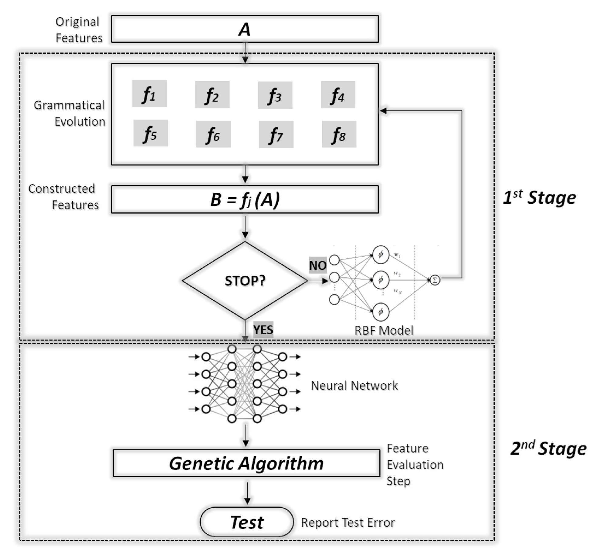
The proposed technique is divided into two phases. During the first phase, artificial new features are created from the original ones using grammatical evolution and a genetic algorithm. The new features are evaluated using a radial basis function (RBF) network [31] with H processing units. The RBF network is selected as the evaluator because the training procedure of RBF is much faster than those of artificial neural networks. Subsequently, in the second phase, the original dataset is transformed using the best located features and a genetic algorithm is used to train a neural network on the modified dataset. A schematic representation of the whole process is shown in Figure 1.
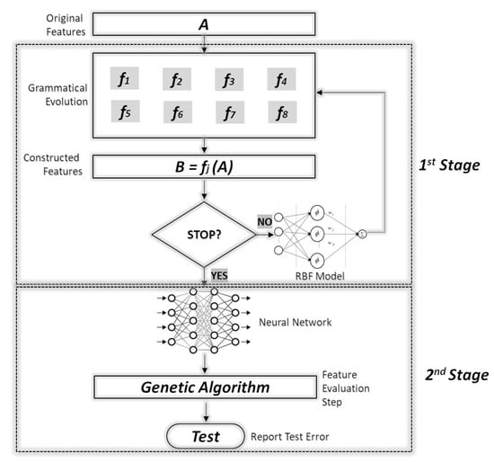
Figure 1.
Flowchart of the proposed algorithm.
2.1. Grammatical Evolution
Grammatical evolution is an evolutionary approach, where the chromosomes are random numbers standing for production rules of a given BNF (Backus–Naur form) grammar [32]. The grammatical evolution was initially used for regression [33,34] and to solve trigonometric identities [35], but it has been applied in a variety of scientific fields, such as the automatic composition of music [36], neural network construction [37,38], automatic constant creation [39], the evolution of video games [40,41], energy-demand estimation [42], combinatorial optimization [43], and cryptography [44]. The BNF grammar is defined as the set where
- N is the set of the non-terminal symbols, used to produce a series of terminal symbols through production rules.
- T is the set of terminal symbols of grammar. For example, terminal symbols could be the digits in an arithmetic expression of the operators.
- S is the starting non-terminal symbol of grammar. The production of a valid expression is initiated from this symbol.
- P is the set of production rules. Every rule is in the form or .
The original grammar is expanded in grammatical evolution, with the addition of a sequence number for each production rule. The chromosomes in grammatical evolution are integer numbers representing sequence numbers of production rules. Subsequently, the production procedure starts from the start symbol of the grammar and produces valid programs by replacing non-terminal symbols with the right hand of the selected production rule. The selection of the rule has two steps:
- Retrieve the next element from the given chromosome and denote it as V.
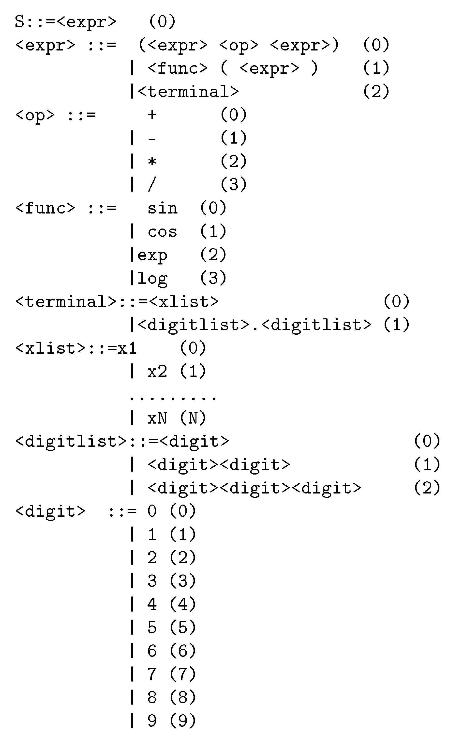
- The next production rule R is calculated bywhere K is the total number of production rules for the current non-terminal symbol. In the current work, the extended BNF grammar is illustrated in Figure 2. The non-terminal symbols are enclosed in the symbols < >, and the number N denotes the number of original features. For the COVID-19 case, N is considered as 1. An example of producing a valid expression is shown in the Table 1. The chromosome is and . The valid expression finally created is .
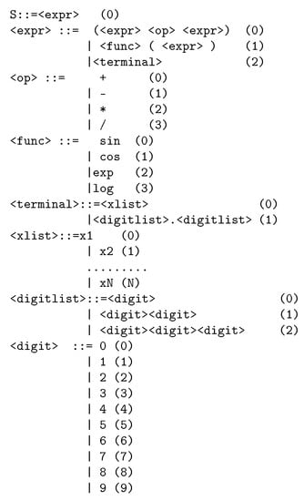 Figure 2. The grammar of the proposed method.
 Table 1. Steps to produce a valid expression from the BNF grammar.
Considering the above mapping procedure, the steps to produce artificial features for a given chromosome g are
- Divide the chromosome into parts. Each part will construct a separate feature.
- A feature is constructed for every using the grammar given in Figure 2.
- Construct a mapping functionwith being the pattern from the original set.
2.2. Feature Creation Step
In this step, a genetic algorithm in conjunction with the mapping procedure of Section 2.1 is used to produce artificial features. The fitness function of the genetic algorithm is the training error of an RBF neural network with H processing units. The steps are as follows:
- Initialization step
- (a)
- Set iter= 0, the current number of generations.
- (b)
- Consider the set , the original training set.
- (c)
- Set as the number of chromosomes in the genetic population.
- (d)
- Set as the number of constructed features.
- (e)
- Initialize randomly in range every element of each chromosome.
- (f)
- Set as the maximum number of generations.
- (g)
- Set as the selection rate.
- (h)
- Set as the mutation rate.
- Termination check step. If iter >= terminate.
- Calculate the fitness of every chromosome with the following procedure:
- (a)
- Create features using the mapping procedure of Section 2.1.
- (b)
- Construct the mapped training set
- (c)
- Train an RBF neural network C with H processing units on the new set and obtain the following training error:
- (d)
- Set
- Genetic Operators
- (a)
- Selection procedure: The chromosomes are sorted according to their fitness. The best are copied intact to the next generation. The genetic operations of crossover and mutation are applied to rest of the chromosomes.
- (b)
- Crossover procedure: During this process , offspring will be created. For every couple of produced offspring, two parents are selected using the well-known procedure of tournament selection. For every pair of parents, two offspring and are produced through one-point crossover. An example of one-point crossover is shown in Figure 3.
 Figure 3. An example of one-point crossover. A randomly selected point is chosen, and the two subparts of the parents are exchanged.
 - (c)
- Mutation procedure: For each element of every chromosome, a random number is produced. Subsequently, we randomly change the corresponding element if .
- Set iter = iter + 1 and goto Step 2.
2.3. Feature Evaluation Step
During this step, the best chromosome of the first step is obtained and used to create the modified train set
Afterwards, a genetic algorithm is used to train an artificial neural network with H hidden nodes for this dataset. The neural network used here is defined as a function , where w is the weight vector to be estimated through the genetic algorithm after the minimization of the following training error:
The neural network has a form also used in [45]. If the neural network has one processing level, every output of each hidden node is in the form:
where is the weight vector and is considered as the bias for output The function is the well-known sigmoid function given by
For a neural network with H hidden nodes, the final output is given by:
where is the weight for hidden node i. Hence, if we use one weight w for hidden nodes and biases, the following form could be used for the neural network:
The value d the size of input vector Additionally, the total number of parameters of vector is . The genetic algorithm used here is a global optimization technique [17,18] that has been applied with success in many problems such as electromagnetic problems [46], combinatorial problems [47], and the design of water distribution networks [48]. Additionally, it has been used to train artificial networks in some works from the relevant literature [49,50,51]. The steps of the genetic algorithm used in the second step of the proposed method are as follows:
- Initialization step.
- (a)
- Set as , the number of chromosomes that will participate.
- (b)
- Set as the maximum number of allowed generations.
- (c)
- Set as , the mutation rate.
- (d)
- Set as the selection rate.
- (e)
- Set, a small positive number, i.e., .
- (f)
- Randomly initialize the chromosomes . For the case of neural networks, every element of each chromosome is considered as a double precision number. Additionally, the size of each chromosome is
- (g)
- Set iter = 0
- Check for termination.
- (a)
- Obtain the best fitness
- (b)
- Terminate if OR
- Calculate fitness.
- (a)
- Fordo
- i.
- Create a neural network using the chromosome as a parameter vector.
- ii.
- Calculate the fitness value using Equation (4).
- (b)
- EndFor
- Application of genetic operators.
- (a)
- Selection operation. During selection, the chromosomes are classified according to their fitness. The first are copied without changes to the next generation of the population. The rest will be replaced by chromosomes that will be produced at the crossover.
- (b)
- Crossover operation. In the crossover operation, chromosomes are produced. For every couple of produced offspring, two parents are selected using tournament selection. For every pair of parents, two offspring and are produced according to the following equations:where is a random number with the property [52].
- (c)
- Mutation operation. For each element of every chromosome, a random number is produced, and the element is altered if .
- (d)
- Set iter = iter + 1.
- Goto step 2.
3. Experimental Results
The data were freely available from the https://ourworldindata.org/explorers/coronavirus-data-explorer (accessed on 10 September 2022), and were downloaded for the start of the pandemic until 10 September 2022. To enable the machine-learning models to better fit the data, the following fair normalization took place in every dataset.
- The number of cases was divided by .
- The number of deaths was divided by .
The following countries were selected for testing: Algeria, Argentina, Australia, Brazil, Bulgaria, Canada, Germany, Greece, Egypt, and Japan. For every country, two distinct datasets were obtained from the COVID-19 database, one dataset for the number of cases on every day of the pandemic and one dataset for the number of deaths on every day of the pandemic. Every run was executed 30 times for every dataset, and averages were measured. The random-number generator used was the drand48() of the C programming language. The parameters for the proposed method are listed in Table 2. The results for the COVID-19 cases are shown in the Table 3, and the results for the COVID-19 deaths are illustrated in Table 4. The columns in both tables have the following meaning:
- The column COUNTRY contains the name of the country.
- The column ADAM stands for the Adam optimization method [53] used to train a neural network with 10 processing nodes. The ADAM method is implemented in OptimLib, and it is available from https://github.com/kthohr/optim (accessed on 10 September 2022).
- The column MLPPSO represents the results using a neural network trained with the help of Particle Swarm Optimization method [54,55]. The number of PSO particles was set to , and the maximum number of allowed iterations was set to . The values for thes parameters are shown in the Table 2. Additionally, the BFGS method [56] was applied to the best particle of the swarm when the PSO finished, in order to enhance the results.
- The column MLPGEN stands for the results obtained by a neural network with ten processing units that was trained using a genetic algorithm [17,18]. The parameters for this algorithm are listed in the Table 2. Additionally, the BFGS was applied to the best chromosome after the termination of the genetic algorithm.
- The column FC1 stands for the results obtained by the proposed method with one constructed feature .
- The column FC2 stands for the results obtained by the proposed method with two constructed features .
- The column FC3 stands for the results obtained by the proposed method with three constructed features .

Table 2.
Experimental parameters.
Table 2.
Experimental parameters.
| Parameter | Value |
|---|---|
| 500 | |
| 200 | |
| H | 10 |
| 0.10 | |
| 0.05 | |

Table 3.
Total test error for the prediction of COVID-19 cases.
Table 3.
Total test error for the prediction of COVID-19 cases.
| Country | ADAM | MLPPSO | MLPGEN | FC1 | FC2 | FC3 |
|---|---|---|---|---|---|---|
| Algeria | 0.31 | 0.08 | 0.286 | 0.0025 | 0.0006 | 0.0002 |
| Argentina | 178.60 | 21.03 | 69.20 | 3.21 | 0.81 | 0.91 |
| Australia | 144.46 | 20.33 | 30.96 | 1.52 | 0.37 | 0.34 |
| Brazil | 198.26 | 81.94 | 75.79 | 11.93 | 8.97 | 6.50 |
| Bulgaria | 4.01 | 1.29 | 2.67 | 0.037 | 0.0098 | 0.01 |
| Canada | 27.68 | 6.12 | 20.65 | 0.33 | 0.20 | 0.15 |
| Germany | 274.34 | 135.15 | 92.50 | 25.05 | 25.11 | 14.36 |
| Greece | 25.07 | 12.08 | 9.25 | 3.62 | 1.60 | 2.75 |
| Egypt | 0.24 | 0.13 | 0.44 | 0.005 | 0.029 | 0.003 |
| Japan | 271.11 | 95.56 | 75.76 | 8.92 | 2.15 | 1.82 |
| Average | 112.41 | 37.37 | 37.75 | 5.46 | 3.92 | 2.68 |

Table 4.
Predicted deaths per country.
Table 4.
Predicted deaths per country.
| Country | ADAM | PSOGEN | MLPGEN | FC1 | FC2 | FC3 |
|---|---|---|---|---|---|---|
| Algeria | 0.40 | 0.15 | 0.66 | 0.009 | 0.002 | 0.002 |
| Argentina | 18.50 | 19.70 | 25.81 | 2.03 | 1.35 | 1.70 |
| Australia | 1.69 | 0.44 | 1.00 | 0.05 | 0.03 | 0.03 |
| Brazil | 416.54 | 282.46 | 230.52 | 52.42 | 16.75 | 16.57 |
| Bulgaria | 3.80 | 2.76 | 16.50 | 0.15 | 0.10 | 0.08 |
| Canada | 9.12 | 4.78 | 18.12 | 0.27 | 0.15 | 0.15 |
| Germany | 116.56 | 37.06 | 40.49 | 3.03 | 2.07 | 4.17 |
| Greece | 3.29 | 2.97 | 2.86 | 0.74 | 0.08 | 0.07 |
| Egypt | 2.57 | 0.79 | 8.88 | 0.07 | 0.03 | 0.02 |
| Japan | 43.10 | 22.07 | 13.74 | 0.32 | 0.12 | 0.13 |
| Average | 61.56 | 37.32 | 35.86 | 5.91 | 2.07 | 2.29 |
Additionally, in both tables, an additional row was added to indicate the average error and is denoted by AVERAGE. This extra column is graphically plotted in Figure 4 and Figure 5 for case predictions and deaths prediction, respectively.
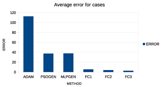
Figure 4.
Graphical representation of average error for predicting COVID-19 cases.
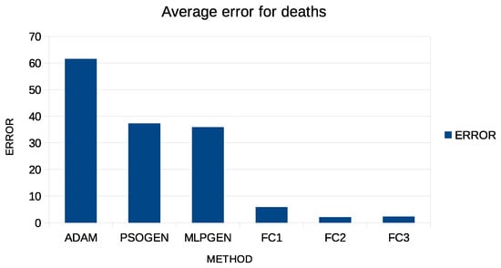
Figure 5.
Graphical representation of average error for predicting COVID-19 deaths.
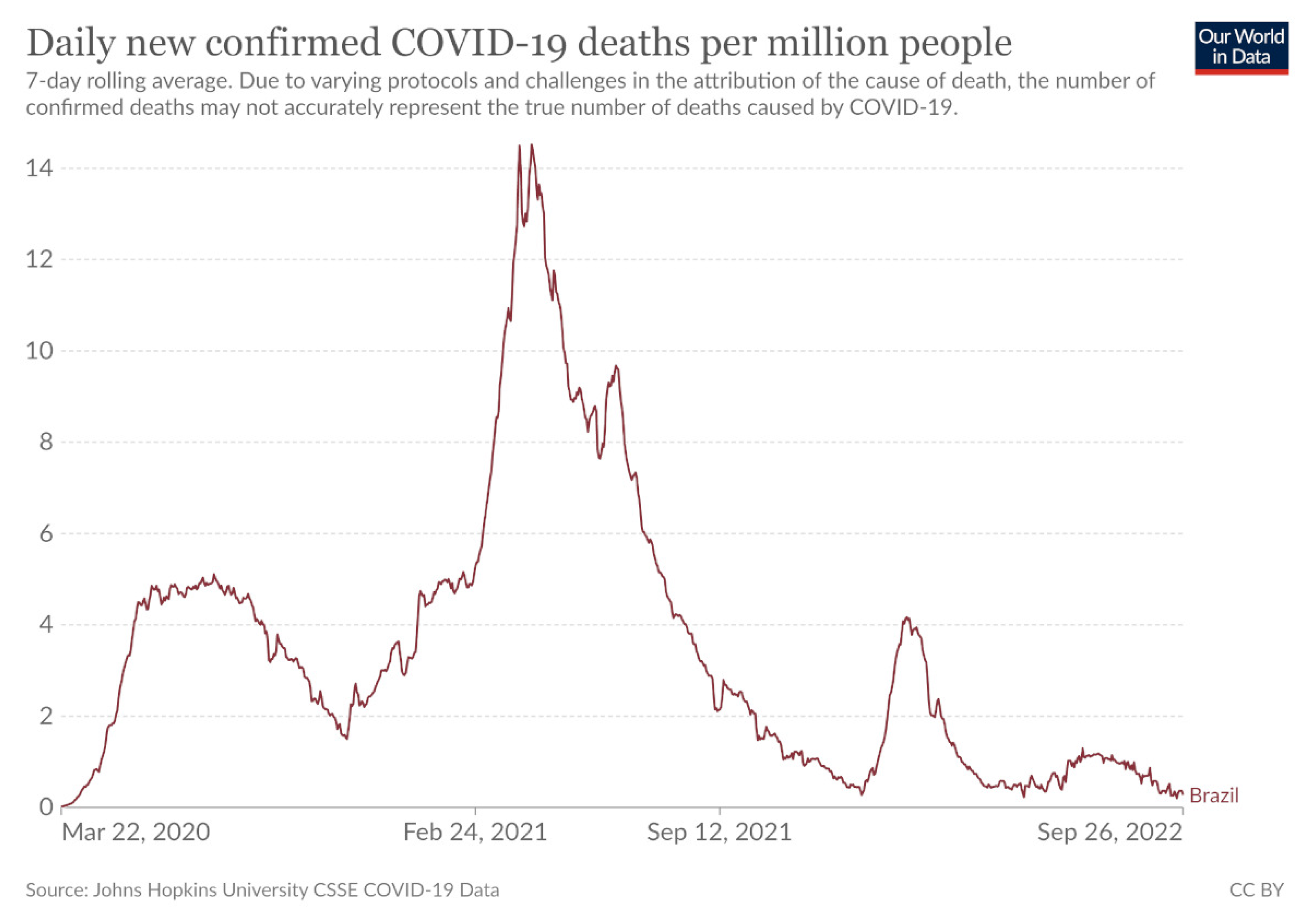
From the execution of the above experiments, it is clear in principle that the efficiency of the methods depends to a great extent on the country in question. In some countries, the test error is high, and in others it’s quite low. This is probably due to the different courses of the number of cases and the mortality rate in each country. For example, if one looks at the experimental results for Brazil, one will find that all the methods present a relatively high error. This may be due to the large and abrupt changes that the disease has caused in this country, as shown in Figure 6, which shows the course of deaths in this country and is available from Johns Hopkins University. However, even in this country using the proposed methodology, there was a large reduction in approximation error of 90%.
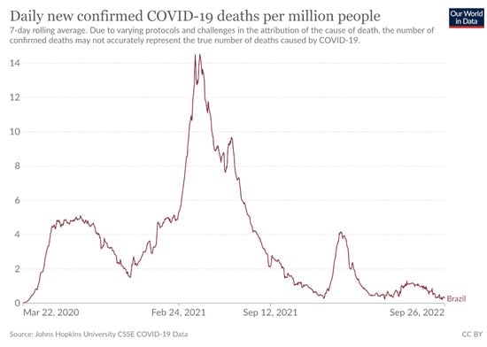
Figure 6.
The daily confirmed deaths for Brazil, available from John Hopkins University.
Moreover, the proposed method has higher accuracy than the other techniques, even if only one artificial feature is created. In fact, in some countries, the test error of the proposed technique is so low that it is almost zero. Using more than one feature appears to drastically reduce the error, although the reduction appears to be more significant between one and two features and less when a third constructed feature is added. Additionally, the Adam method appears to achieve worse results than the PSO and the genetic algorithm methods, and this is expected since this method is a local optimization technique, while the PSO and the genetic algorithms are global optimization methods.
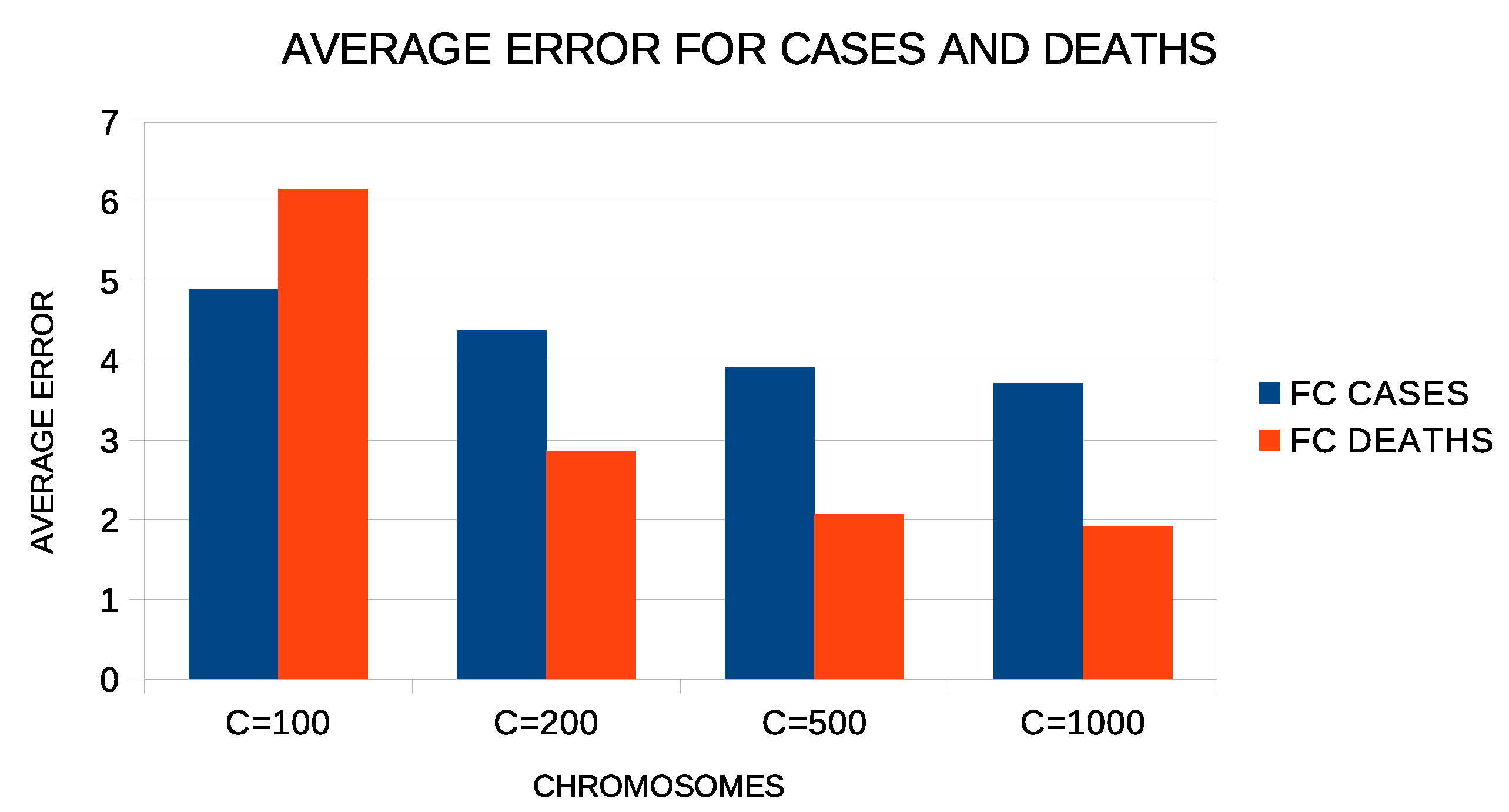
Additional experiments were performed to evaluate the parameters used in the proposed method. Figure 7 shows the average error of the proposed method with two constructed features for all experiment countries. In these experiments, a varying number of chromosomes was used from 100 to 1000. As expected, the proposed method reduces the average error as the number of chromosomes increases. This means, however, that the execution time of the method increases as well as the memory that will be needed to store the computational structures. Therefore, the value of 500 used in the proposed method for the number of chromosomes is a good compromise between the speed and efficiency of the proposed technique.
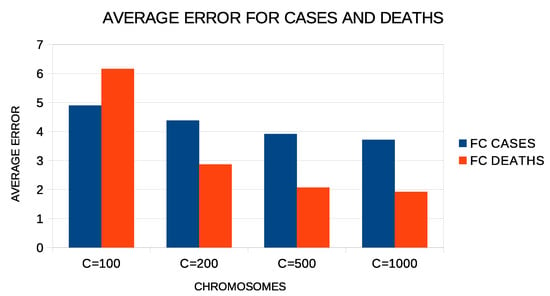
Figure 7.
Average test error for COVID-19 cases and deaths for different numbers of chromosomes and two constructed features.
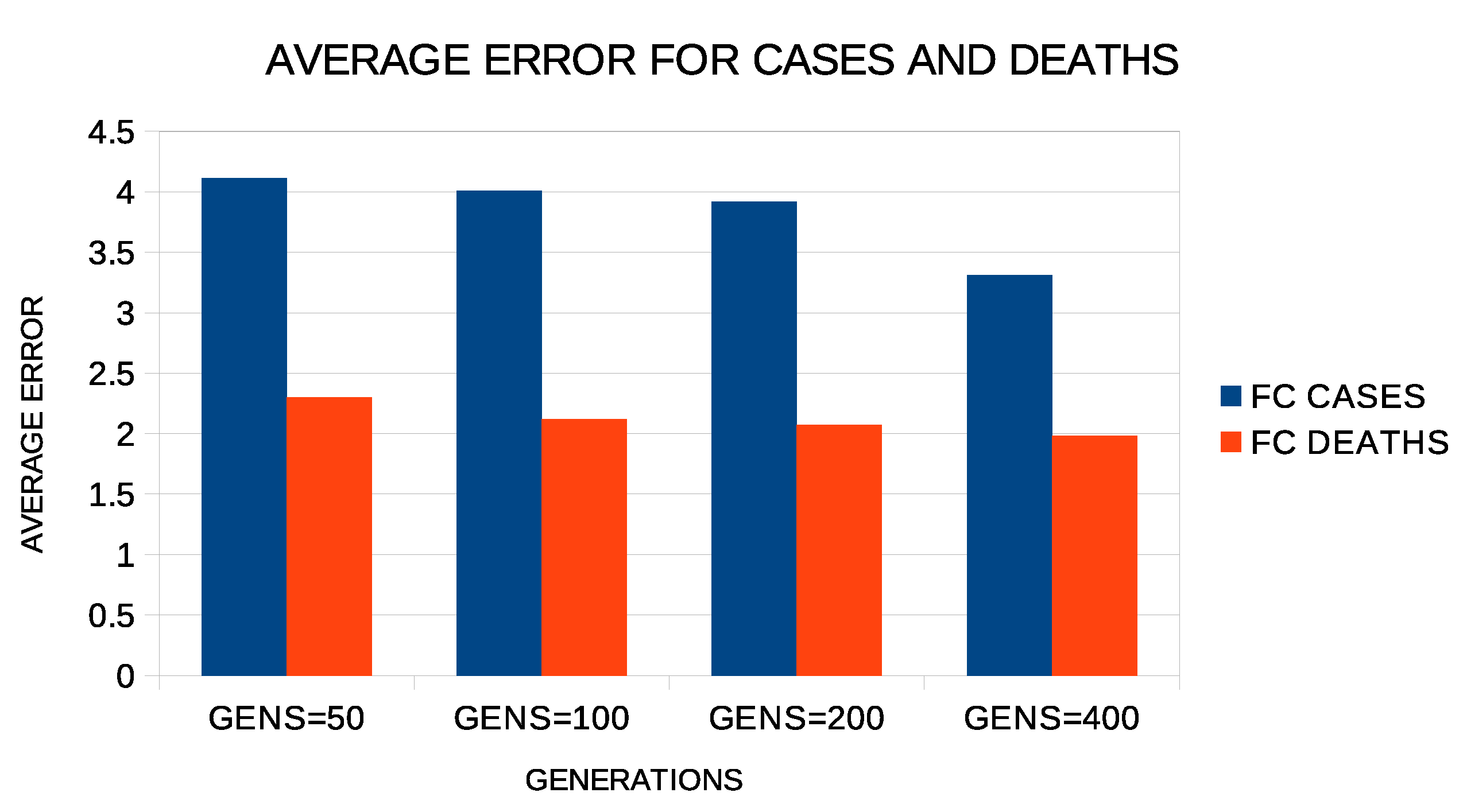
Regarding the number of generations of the genetic algorithm, similar experiments were carried out with this number between 50 and 400. The results of these experiments are shown in Figure 8. Again, increasing the number of generations seems to reduce the error, although the reduction is not as drastic as it was with the increase in chromosomes. Again, the choice of 200 made for the number of generations in the experiments appears to be a fair compromise.

Figure 8.
Average test error for COVID-19 cases and deaths for different numbers of generations and two constructed features.
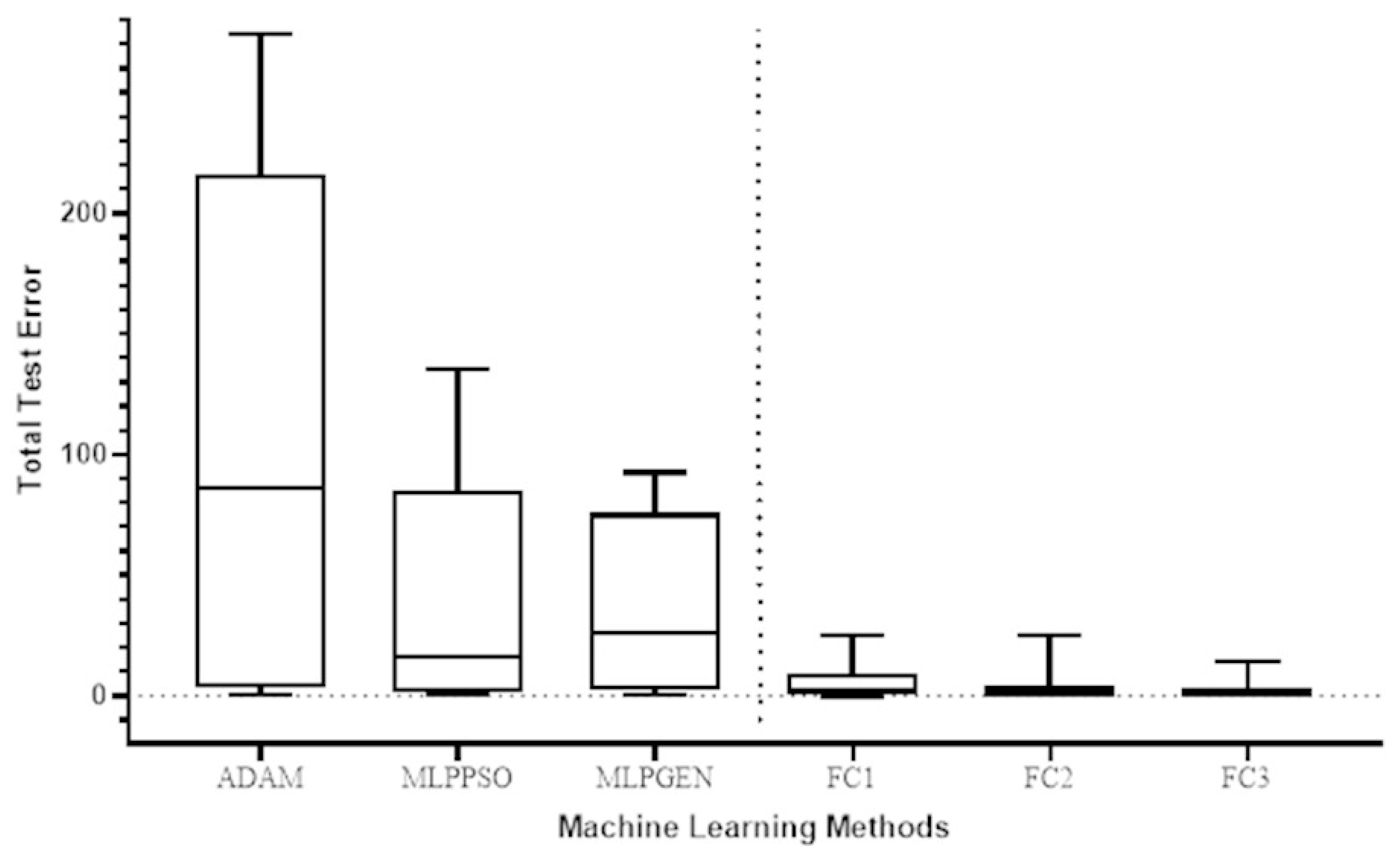
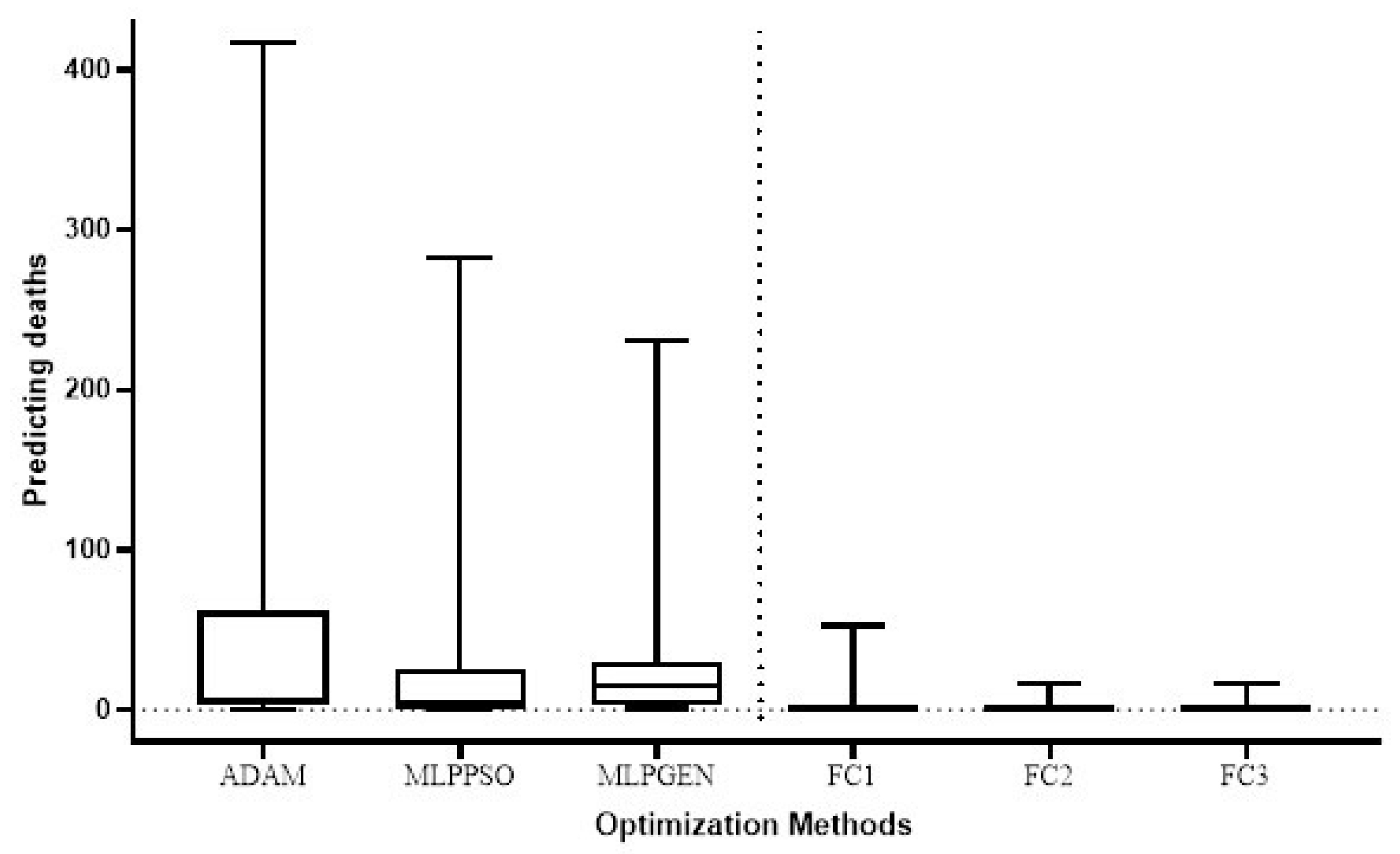
The Wilcoxon signed-rank test was used to compare the total test error for the prediction of COVID-19 cases in different countries of the proposed method (FC1, FC2, and FC3) with the respective total test error for the ADAM, MLPPSO, and MLPGEN optimization methods. The results obtained through those statistical tests are shown in Figure 9. We also compared the average error in predicting deaths per country of the proposed method (FC1, FC2, and FC3) with the average error for ADAM, MLPPSO, and MLPGEN optimization methods using the Wilcoxon signed-rank test. The results obtained through those statistical tests are shown in Figure 10.

Figure 9.
Box plot comparing the total test error for predicting COVID-19 cases among the optimization methods of different countries.

Figure 10.
Box plot comparing the average error in predicting deaths per country among the optimization methods.
4. Conclusions
In this paper, the use of a feature-construction technique to predict the cases of COVID19 disease and to predict the mortality due to it was presented. The prediction was made on widely available data for 10 randomly selected countries. The proposed method constructs new features from existing ones using grammatical evolution and evaluates them using a radial basis network (RBF). After the evaluation, the best resulting features are used to train an artificial neural network. The results of the proposed methodology were compared with those of other artificial neural network training techniques, and in all cases there was a dramatic reduction in the network’s error for both case-number prediction and mortality prediction. Furthermore, the more artificial features that are created, the lower the neural network error. Future research should include the physical interpretation of the generated features in relation to the nature of the problem. Additionally, future improvements to the method may include:
- The incorporation of more advanced stopping rules for the genetic algorithms of the two phases.
- The usage of other machine-learning models instead of the RBF network, to evaluate the constructed features.
- The usage of parallel techniques to speed up the feature-creation process.
- The use of a data technique that will also contain the demographic characteristics of each country, in order to establish whether there is a correlation of the rate of cases or mortality with the particular characteristics of some countries.
Author Contributions
I.G.T., A.T.T. and D.T. conceived the idea and methodology and supervised the technical part regarding the software. I.G.T. conducted the experiments, employing several datasets, and provided the comparative experiments. A.T.T. performed the statistical analysis. D.T. and all other authors prepared the manuscript. D.T. and I.G.T. organized the research team and A.T.T. supervised the project. All authors have read and agreed to the published version of the manuscript.
Funding
We acknowledge support of this work from the project “Immersive Virtual, Augmented and Mixed Reality Center of Epirus” (MIS 5047221) which is implemented under the Action “Reinforcement of the Research and Innovation Infrastructure”, funded by the Operational Programme “Competitiveness, Entrepreneurship and Innovation” (NSRF 2014-2020) and co-financed by Greece and the European Union (European Regional Development Fund).
Data Availability Statement
Not applicable.
Acknowledgments
We acknowledge support of this work from the project “Immersive Virtual, Augmented and Mixed Reality Center of Epirus” (MIS 5047221) which is implemented under the Action “Reinforcement of the Research and Innovation Infrastructure”, funded by the Operational Programme “Competitiveness, Entrepreneurship and Innovation” (NSRF 2014-2020) and co-financed by Greece and the European Union (European Regional Development Fund).
Conflicts of Interest
The authors declare no conflict of interest.
References
- Andersen, K.G.; Rambaut, A.; Lipkin, W.I.; Holmes, E.C.; Garry, R.F. The proximal origin of sars-cov-2. Nat. Med. 2020, 26, 450–452. [Google Scholar] [CrossRef] [PubMed]
- Wang, L.; Li, J.; Guo, S.; Xie, N.; Yao, L.; Cao, Y.; Day, S.W.; Howard, S.C.; Gra, J.C.; Gu, T.; et al. Real-time estimation and prediction of mortality caused by covid-19 with patient information based algorithm. Sci. Total Environ. 2020, 727, 138394. [Google Scholar] [CrossRef] [PubMed]
- Tomar, A.; Gupta, N. Prediction for the spread of covid- 19 in india and eectiveness of preventive measures. Sci. Total Environ. 2020, 728, 138762. [Google Scholar] [CrossRef] [PubMed]
- Zhang, X.; Ma, R.; Wang, L. Predicting turning point, duration and attack rate of covid-19 outbreaks in major western countries. Chaos Solitons Fractals 2020, 135, 109829. [Google Scholar] [CrossRef] [PubMed]
- Pinter, G.; Felde, I.; Mosavi, A.; Ghamisi, P.; Gloaguen, R. COVID-19 pandemic prediction for hungary; a hybrid machine learning approach. Mathematic 2020, 8, 890. [Google Scholar]
- Smith, M.; Alvarez, F. Identifying mortality factors from machine learning using shapley values a case of covid19. Expert. Appl. 2021, 176, 114832. [Google Scholar] [CrossRef] [PubMed]
- Loey, M.; Manogaran, G.; Taha, M.H.N.; Khalifa, N.E.M. A hybrid deep transfer learning model with machine learning methods for face mask detection in the era of the covid-19 pandemic. Measurement 2021, 167, 108288. [Google Scholar] [CrossRef]
- Mundial, I.Q.; Ul Hassan, M.S.; Tiwana, M.I.; Qureshi, W.S.; Alanazi, E. Towards facial recognition problem in COVID-19 pandemic. In Proceedings of the 2020 4rd International Conference on Electrical, Telecommunication and Computer Engineering (ELTICOM), Medan, Indonesia, 3–4 September 2020; pp. 210–214. [Google Scholar]
- Gavrilis, D.; Tsoulos, I.G.; Dermatas, E. Selecting and constructing features using grammatical evolution. Pattern Recognit Lett. 2008, 29, 1358–1365. [Google Scholar]
- O’Neill, M.; Ryan, C. grammatical evolution. IEEE Trans. Evol. Comput. 2001, 5, 349–358. [Google Scholar] [CrossRef]
- Gavrilis, D.; Tsoulos, I.G.; Dermatas, E. Neural recognition and genetic features selection for robust detection of e-mail spam. In Hellenic Conference on Articial Intelligence; Springer: Berlin/Heidelberg, Germany, 2006; pp. 498–501. [Google Scholar]
- Georgoulas, G.; Gavrilis, D.; Tsoulos, I.G.; Stylios, C.; Bernardes, J.; Groumpos, P.P. Novel approach for fetal heart rate classication introducing grammatical evolution. Biomed. Signal Process. Control 2007, 2, 69–79. [Google Scholar] [CrossRef]
- Smart, O.; Tsoulos, I.G.; Gavrilis, D.; Georgoulas, G. Grammatical evolution for features of epileptic oscillations in clinical intracranial electroencephalograms. Expert Syst. Appl. 2011, 38, 9991–9999. [Google Scholar] [CrossRef] [PubMed][Green Version]
- Tsoulos, I.G. QFC: A Parallel Software Tool for Feature Construction, Based on grammatical evolution. Algorithms 2022, 15, 295. [Google Scholar] [CrossRef]
- Bishop, C. Neural Networks for Pattern Recognition; Oxford University Press: Oxford, UK, 1995. [Google Scholar]
- Cybenko, G. Approximation by superpositions of a sigmoidal function. Math. Control. Signals Syst. 1989, 2, 303–314. [Google Scholar] [CrossRef]
- Goldberg, D. Genetic Algorithms in Search, Optimization and Machine Learning; Addison-Wesley Publishing Company: Reading, MA, USA, 1989. [Google Scholar]
- Michaelewicz, Z. Genetic Algorithms + Data Structures = Evolution Programs; Springer: Berlin, Germany, 1996. [Google Scholar]
- Ghosh, S.C.; Sinha, B.P.; Das, N. Channel assignment using genetic algorithm based on geometric symmetry. IEEE Trans. Veh. Technol. 2003, 52, 860–875. [Google Scholar] [CrossRef]
- Liu, Y.; Zhou, D. An Improved Genetic Algorithm with Initial Population Strategy for Symmetric TSP. Math. Probl. Eng. 2015, 2015, 212794. [Google Scholar]
- Han, S.; Barcaro, G.; Fortunelli, A.; Lysgaard, S.; Vegge, T.; Hansen, H.A. Unfolding the structural stability of nanoalloys via symmetry-constrained genetic algorithm and neural network potential. npj Comput. Mater. 2022, 8, 121. [Google Scholar] [CrossRef]
- Krippendorf, S.; Syvaeri, M. Detecting symmetries with neural networks. Mach. Learn. Sci. Technol. 2020, 2, 015010. [Google Scholar] [CrossRef]
- Qiao, Z.; Welborn, M.; Anandkumar, A.; Manby, F.R.; Miller, T.F., III. OrbNet: Deep learning for quantum chemistry using symmetry-adapted atomic-orbital features. J. Chem. Phys. 2020, 153, 124111. [Google Scholar] [CrossRef]
- Xi, B.; Tse, K.F.; Kok, T.F.; Chan, H.M.; Chan, H.M.; Chan, M.K.; Chan, H.Y.; Wong, K.Y.C.; Yuen, S.H.R.; Zhu, J. Machine-Learning-Assisted Acceleration on High-Symmetry Materials Search: Space Group Predictions from Band Structures. J. Phys. Chem. C 2022, 126, 12264–12273. [Google Scholar] [CrossRef]
- Selvaratnam, B.; Koodali, R.T.; Miró, P. Application of Symmetry Functions to Large Chemical Spaces Using a Convolutional Neural Network. J. Chem. Inf. Model. 2020, 60, 1928–1935. [Google Scholar] [CrossRef] [PubMed]
- Wang, Z.; Wang, C.; Zhao, S.; Du, S.; Xu, Y.; Gu, B.L.; Duan, W. Symmetry-adapted graph neural networks for constructing molecular dynamics force fields. Sci. China Phys. Mech. Astron. 2021, 64, 117211. [Google Scholar] [CrossRef]
- Tuan, N.H.; Mohammadi, H.; Rezapour, S. A mathematical model for COVID-19 transmission by using the Caputo fractional derivative. Chaos Solitons Fractals 2020, 140, 110107. [Google Scholar] [CrossRef] [PubMed]
- Panwar, V.S.; Uduman, P.S.; Gómez-Aguilar, J.F. Mathematical modeling of coronavirus disease COVID-19 dynamics using CF and ABC non-singular fractional derivatives. Chaos Solitons Fractals 2021, 145, 110757. [Google Scholar] [CrossRef]
- Shaikh, A.S.; Shaikh, I.N.; Nisar, K.S. A mathematical model of COVID-19 using fractional derivative: Outbreak in India with dynamics of transmission and control. Adv. Differ. Equ. 2020, 373. [Google Scholar] [CrossRef] [PubMed]
- Huzaifa, E.; Khan, A.; Shah, M.; Khan, M. Taylor Series Expansion Method To Compute Approximate Solution for Nonlinear Dynamical System. J. Fract. Calc. Nonlinear Syst. 2022, 3, 20–29. [Google Scholar] [CrossRef]
- Park, J.; Sandberg, I.W. Universal Approximation Using Radial-Basis-Function Networks. Neural Comput. 1991, 3, 246–257. [Google Scholar] [CrossRef] [PubMed]
- Backus, J.W. The Syntax and Semantics of the Proposed International Algebraic Language of the Zurich ACM-GAMM Conference. In Proceedings of the International Conference on Information Processing, UNESCO, Paris, France, 15–20 June 1959; pp. 125–132. [Google Scholar]
- Ryan, C.; Collins, J.; O’Neill, M. grammatical evolution: Evolving programs for an arbitrary language. In Genetic Programming. EuroGP 1998; Lecture Notes in Computer Science; Banzhaf, W., Poli, R., Schoenauer, M., Fogarty, T.C., Eds.; Springer: Berlin/Heidelberg, Germany, 1998; Volume 1391. [Google Scholar]
- O’Neill, M.; Ryan, M.C. Evolving Multi-line Compilable C Programs. In Genetic Programming. EuroGP 1999; Lecture Notes in Computer Science; Poli, R., Nordin, P., Langdon, W.B., Fogarty, T.C., Eds.; Springer: Berlin/Heidelberg, Germany, 1999; Volume 1598. [Google Scholar]
- Ryan, C.; O’Neill, M.; Collins, J.J. Grammatical evolution: Solving trigonometric identities. In Proceedings of the Mendel, 4th International Mendel Conference on Genetic Algorithms, Optimization Problems, Fuzzy Logic, Neural Networks, Rough Sets, Brno, Czech Republic, 24–26 June 1998. [Google Scholar]
- Puente, A.O.; Alfonso, R.S.; Moreno, M.A. Automatic composition of music by means of grammatical evolution. In Proceedings of the 2002 Conference on APL: Array Processing Languages: Lore, Problems, and Applications (APL ′02), Madrid, Spain, 22–25 July 2002; pp. 148–155. [Google Scholar]
- De Campos, L.M.L.; de Oliveira, R.C.L.; Roisenberg, M. Optimization of neural networks through grammatical evolution and a genetic algorithm. Expert Syst. Appl. 2016, 56, 368–384. [Google Scholar] [CrossRef]
- Soltanian, K.; Ebnenasir, A.; Afsharchi, M. Modular grammatical evolution for the Generation of Artificial Neural Networks. Evol. Comput. 2022, 30, 291–327. [Google Scholar] [CrossRef]
- Dempsey, I.; O’ Neill, M.; Brabazon, A. Constant creation in grammatical evolution. Int. J. Innov. Appl. 2007, 1, 23–38. [Google Scholar] [CrossRef]
- Galván-López, E.; Swafford, J.M.; O’Neill, M.; Brabazon, A. Evolving a Ms. PacMan Controller Using grammatical evolution. In Applications of Evolutionary Computation. EvoApplications 2010; Lecture Notes in Computer Science; Springer: Berlin/Heidelberg, Germany, 2010; Volume 6024. [Google Scholar]
- Shaker, N.; Nicolau, M.; Yannakakis, G.N.; Togelius, J.; O’Neill, M. Evolving levels for Super Mario Bros using grammatical evolution. In Proceedings of the 2012 IEEE Conference on Computational Intelligence and Games (CIG), Granada, Spain, 11–14 September 2012; pp. 304–331. [Google Scholar]
- Martínez-Rodríguez, D.; Colmenar, J.M.; Hidalgo, J.I.; Villanueva Micó, R.J.; Salcedo-Sanz, S. Particle swarm grammatical evolution for energy demand estimation. Energy Sci. Eng. 2020, 8, 1068–1079. [Google Scholar] [CrossRef]
- Sabar, N.R.; Ayob, M.; Kendall, G.; Qu, R. Grammatical Evolution Hyper-Heuristic for Combinatorial Optimization Problems. IEEE Trans Evol. Comput. 2013, 17, 840–861. [Google Scholar] [CrossRef]
- Ryan, C.; Kshirsagar, M.G.; Vaidya, G.; Cunningham, A.; Sivaraman, R. Design of a cryptographically secure pseudo random number generator with grammatical evolution. Sci. Rep. 2022, 12, 8602. [Google Scholar] [CrossRef] [PubMed]
- Tsoulos, I.G.; Gavrilis, D.; Glavas, E. Neural network construction and training using grammatical evolution. Neurocomputing 2008, 72, 269–277. [Google Scholar] [CrossRef]
- Haupt, R.L. An introduction to genetic algorithms for electromagnetics. Antennas Propag. Mag. 1995, 37, 7–15. [Google Scholar] [CrossRef]
- Grefenstette, J.J.; Gopal, R.; Rosmaita, B.J.; Van Gucht, D. Genetic Algorithms for the Traveling Salesman Problem. In Proceedings of the 1st International Conference on Genetic Algorithms, Pittsburgh, PA, USA, 24–26 July 1985; pp. 160–168. [Google Scholar]
- Savic, D.A.; Walters, G.A. Genetic Algorithms for Least-Cost Design of Water Distribution Networks. J. Water Resources Plan. Manag. 1997, 123, 67–77. [Google Scholar] [CrossRef]
- Leung, F.H.F.; Lam, H.K.; Ling, S.H.; Tam, P.K.S. Tuning of the structure and parameters of a neural network using an improved genetic algorithm. IEEE Trans. Neural Netw. 2003, 14, 79–88. [Google Scholar] [CrossRef] [PubMed]
- Sedki, A.; Ouazar, D.; El Mazoudi, E. Evolving neural network using real coded genetic algorithm for daily rainfall–runoff forecasting. Expert Syst. Appl. 2009, 36, 4523–4527. [Google Scholar] [CrossRef]
- Majdi, A.; Beiki, M. Evolving neural network using a genetic algorithm for predicting the deformation modulus of rock masses. Int. J. Rock Mech. Min. Sci. 2010, 47, 246–253. [Google Scholar] [CrossRef]
- Kaelo, P.; Ali, M.M. Integrated crossover rules in real coded genetic algorithms. Eur. J. Oper. 2007, 176, 60–76. [Google Scholar] [CrossRef]
- Kingma, D.P.; Ba, J.L. ADAM: A method for stochastic optimization. In Proceedings of the 3rd International Conference on Learning Representations (ICLR 2015), San Diego, CA, USA, 7–9 May 2015; pp. 1–15. [Google Scholar]
- Kennedy, J.; Eberhart, R.C. The particle swarm: Social adaptation in information processing systems. In New Ideas in Optimization; Corne, D., Dorigo, M., Glover, F., Eds.; McGraw-Hill: Cambridge, UK, 1999; pp. 11–32. [Google Scholar]
- Marini, F.; Walczak, B. Particle swarm optimization (PSO). A tutorial. Chemom. Intell. Lab. Syst. 2015, 149, 153–165. [Google Scholar] [CrossRef]
- Powell, M.J.D. A Tolerant Algorithm for Linearly Constrained Optimization Calculations. Math. Program. 1989, 45, 547–566. [Google Scholar] [CrossRef]
Publisher’s Note: MDPI stays neutral with regard to jurisdictional claims in published maps and institutional affiliations. |
© 2022 by the authors. Licensee MDPI, Basel, Switzerland. This article is an open access article distributed under the terms and conditions of the Creative Commons Attribution (CC BY) license (https://creativecommons.org/licenses/by/4.0/).

