Seismic Response Analysis of Uplift Terrain under Oblique Incidence of SV Waves

Abstract

In order to analyze the impact of seismic waves on the venue earthquake, based on the display finite element method, the viscoelastic artificial boundary is used to analyze the variation of the ground motion amplification coefficient and the Fourier spectrum of the raised terrain under different incident angles with SV wave oblique incidence on different slopes. This verification model analysis solution and numerical solution are better. The numerical simulation results show that as the degree of the slope increases, the seismic amplification coefficient increases, and its slope amplification coefficient changes significantly. The X direction coefficient is greater than Y’s magnification coefficient. The Fourier curve with a frequency of 0.2~1 Hz increases with the slope of the raised terrain; when the El Centro is incorporated at 30°, the Fourier spectrum amplitude decreases as the incident angle increases in the low-frequency band. The amplitude of the Fourier spectrum at the high-frequency band monitoring point changes with the incident angle. In the high-frequency band from 1 to 10 Hz, the rate of amplitude change is the largest. When the incident angle is at 0°, the amplification coefficient in the Y direction is basically symmetric.

1. Introduction

A large number of studies have shown that various irregular terrains have a certain influence on ground motions [1,2,3], such as raised terrain, river valley terrain, ridge, etc. The site effect has theoretical research and numerical analysis. Trifunac [4] studied the scattering of SH wave by canyon. The different incident angles of seismic waves correspond to the different seismic responses of soil. It is suggested that when the wavelength of the incident wave is smaller than the radius of a canyon, topography will have a significant effect on the incident wave. Tsaur [5] studied the scattering effect of an SH wave by elliptic protection topography, applied a series to solve the problem, and expressed the wave field by elliptic coordinate separation variables. The focusing effect is analyzed in the frequency domain and it is concluded that the geometric structure can cause the local amplification effect of seismic waves. Zhang [6] analyzed the effects of P, SV and Rayleigh waves on the seismic response of canyon topography by using complex functions, deduced the solution formula, obtained the scattered wave potential energy by using image methods, and studied the effects of canyon geometry and material parameters on the seismic response. Ba Zhenning [7] applied the boundary element method (IBEM) to analyze the influence of a basin on shear wave and longitudinal wave scattering. By solving Green’s function, it was found that the geometric size and material parameters of a basin and the incident angle of an incident wave had a significant influence on the seismic response of a basin. Wong [8] analyzed the impact of the incident angle, valley width and seismic wave wavelength on valley earthquakes by analyzing the scattering of SH waves from a semielliptical valley. For short incident waves, surface displacement amplitudes change rapidly from one point to another, while for the long waves and shallow canyons, displacement amplitudes display only a minor departure from the uniform half-space amplification. Akira Ohtsuki [9] studied the response of an SV wave incident on uneven ground to ground motion, using a combination of a particle model and finite element method (FEM) to calculate and verify the accuracy of the calculation results. The research results show that the incident wavelength, terrain and the feature size have a great influence on the slope displacement and magnification phenomenon. Yuan [10] used the wave function expansion method to study the scattering of plane SH waves by elastic half-space cylindrical hills. The frequency, incidence angle and radius ratio of seismic waves have obvious effects on ground motions. Tsaur [11] used the wave function expansion method to calculate the series solution, simplified the calculation formula of the semicircle, discussed the steady state of the parameters, and obtained the calculation results in the frequency domain. For the seismic dynamic response, most studies only study the vertical incidence of seismic waves, but the seismic dynamic response is more serious under oblique incidence. Fan [12] analyzed the dynamic response of rock slopes under different incident angles of seismic waves based on the viscous boundary. Yin [13] studied the oblique incidence of shear waves. The corresponding program for the development of the viscoelastic boundary was Abaqus software, which allows the input of seismic waves, and then the correctness of the method can be proved by numerical examples. The influence of the change of the incident angle of seismic waves on the seismic response was studied.

In this paper, the viscoelastic boundary condition is applied; the corresponding MATLAB program is compiled; the seismic wave is input in the form of the equivalent nodal load; and the input file is modified through the secondary development of Abaqus. The distribution of ground motions and the amplification effect on the site under the oblique incidence of SV waves are analyzed.

2. Methodology

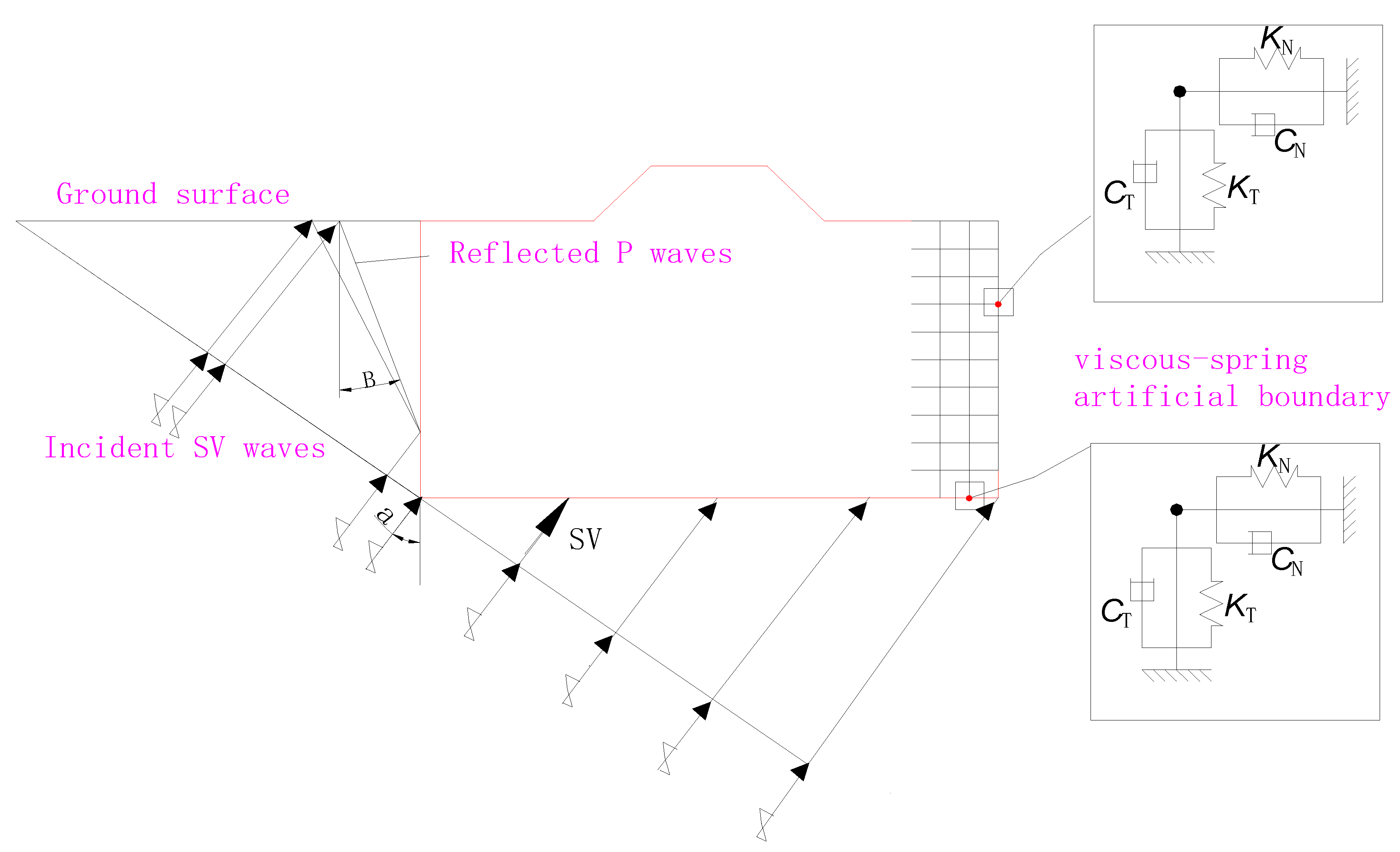
2.1. Establishment of Artificial Boundary

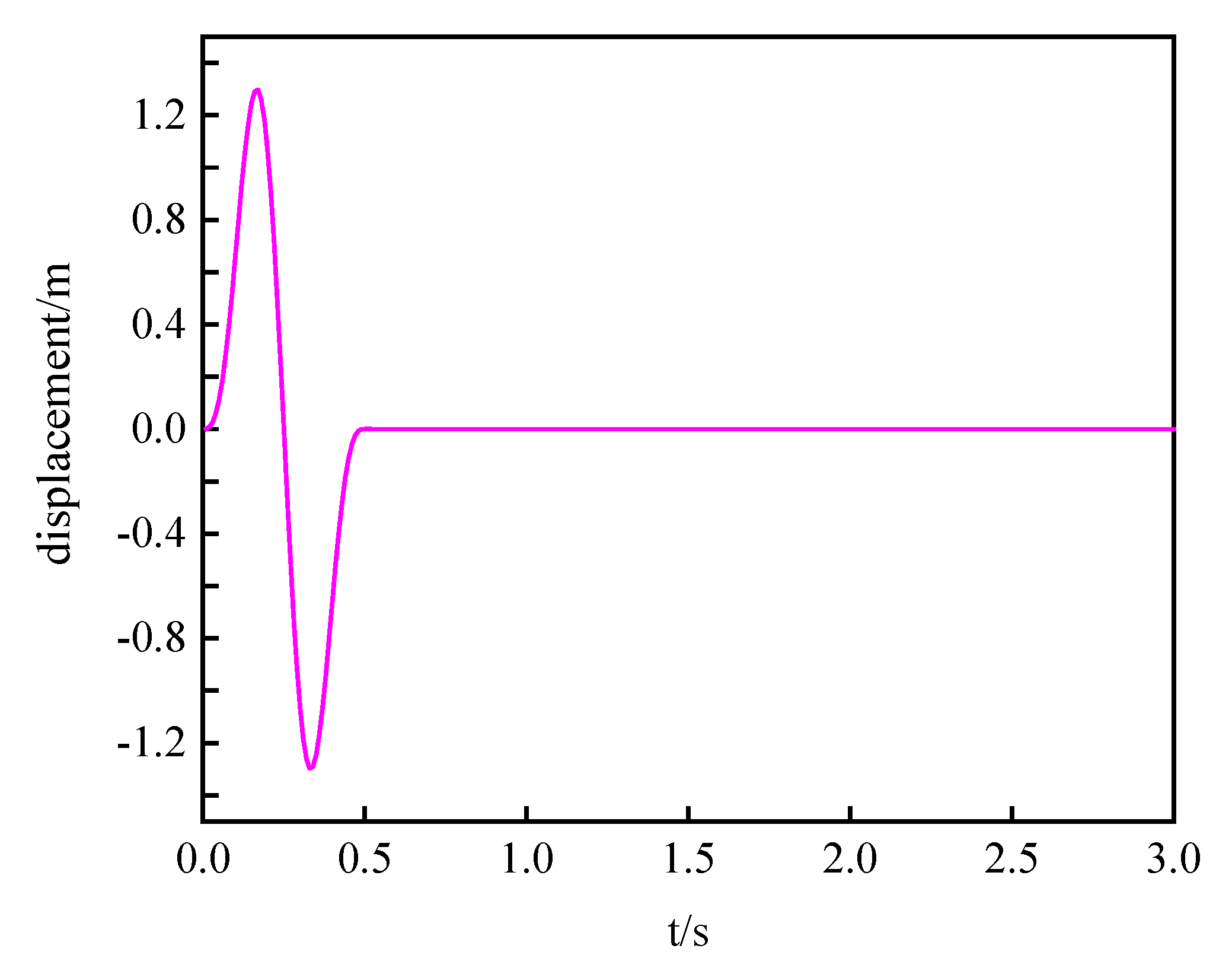
A viscous-spring artificial boundary can absorb the energy radiated from the computing area. This boundary is a good model for the effect of infinite foundations on the computational area. In a two-dimensional viscoelastic artificial boundary, spring and damping elements should be installed in both directions of each node on the boundary of the finite element model. Relevant studies [14] have shown that the accuracy of the viscoelastic boundary is relatively high, and the recovery force of soil in the later stage is relatively good. At the boundary nodes of the FEM model, elastic springs and dampers are established in parallel to implement the viscous-spring artificial boundary, as illustrated in Figure 1. Here, $K$ is the coefficient of the elastic spring, and $C$ is the coefficient of the damper, which can be defined as follows.

$$K_{\mathrm{N}}=\frac{1}{1+A}\cdot \frac{\lambda +2G}{R}\cdot A_l, C_{\mathrm{N}}=B\rho c_p\cdot A_l$$

(1)

$$K_{\mathrm{T}}=\frac{1}{1+A}\frac{G}{R}\cdot A_l, C_{\mathrm{T}}=B\rho c_s\cdot A_l$$

(2)

where the subscripts N and T represent the normal direction and tangential direction, respectively. $R$ indicates the distance from the scattered wave source to the artificial boundary; $c_p$ and $c_s$ are the velocities of the compression wave and shear wave in the medium, respectively. $G$ is the shear modulus; $\rho$ is the mass density; and A and B are the modified coefficients, where good values for the coefficients are 0.8 and 1.1, respectively [15]. $A_l$ represents the influence area of the artificial boundary on each node, for example, at node $l$, $A_l=(A_1+A_2)/2$, and the seismic wave oblique incidence model is depicted in Figure 1.

2.2. Input Method

The total wavefield motion equation of the finite element time-domain method is shown as:

$$m_1{\ddot{u}}_{li}+{\displaystyle \sum _{k=1}^{n_e}{\displaystyle \sum _{j=1}^n{c}_{likj}}}{\dot{u}}_{kj}+{\displaystyle \sum _{k=1}^{n_e}{\displaystyle \sum _{j=1}^n{k}_{likj}}}{u}_{kj}=A_l{\sigma }_{li}$$

(3)

$m_l$ is the mass of the node; $k_{likj}$ is the stiffness of node $k$ direction $j$ to node $l$ direction $i$; $c_{likj}$ is the damping coefficient; $u_{kj}$ is the displacement of node $k$ direction $j$; ${\dot{u}}_{kj}$ is the speed; ${\ddot{u}}_{li}$ is the acceleration; ${\sigma }_{li}$ is the force exerted by the infinite far field at $i$ in the direction of node $l$ on the finite near field; and $A_l$ is the influence area of the node.

The free field and the scattered field form the total wave field.

$$u_{li}=u_{li}{}^f+u_{li}{}^s$$

(4)

$${\sigma }_{li}={\sigma }_{li}{}^f+{\sigma }_{li}{}^s$$

(5)

$u_{li}{}^f$ is the displacement of the free field or internal field; $u_{li}{}^s$ is the scattered field or the lay field displacement. The stress relation of the artificial boundary point is

$${\sigma }_{li}{}^s=-k_{li}{u}_{li}{}^s-c_{li}{\dot{u}}_{li}{}^s$$

(6)

$k_{li}$ and $c_{li}$ are viscoelastic boundary parameters.

The finite element equations of motion for viscoelastic boundary are obtained

$$m_1{\ddot{u}}_{li}+{\displaystyle \sum _{k=1}^{n_e}{\displaystyle \sum _{j=1}^n(c_{likj}}}+{\delta }_{lk}{\delta }_{ij}{A}_l{c}_{li}){\dot{u}}_{kj}+{\displaystyle \sum _{k=1}^{n_e}{\displaystyle \sum _{j=1}^n(k_{likj}+{\delta }_{lk}{\delta }_{ij}{A}_l{c}_{li})}}{u}_{kj}=A_l({\sigma }_{li}{k}_{li}{u}_{li}{}^f+c_{li}{\dot{u}}_{li}{}^f+{\sigma }_{li}{}^f)$$

(7)

The problem of ground motion input is transformed into the problem of equivalent nodal force on the artificial boundary surface.

Plane SV wave incident at angle $\alpha$ generates SV wave with reflection angle $\alpha$ and P wave with reflection angle $\beta$. The reflection angle and reflected wave amplitude are

$${\beta }_p=\arcsin (\frac{c_p\sin \alpha }{c_s})$$

(8)

$$A_1=\frac{c_s^2\sin 2\alpha \sin 2{\beta }_p-c_p^2{\cos }^{2}2\alpha }{c_s^2\sin 2\alpha \sin 2{\beta }_p+c_p^2{\cos }^{2}2\alpha }$$

(9)

$$A_2=\frac{2c_p{c}_s\sin 2\alpha \cos 2\alpha }{c_s^2\sin 2\alpha \sin 2{\beta }_p+c_p^2{\cos }^{2}2\alpha }$$

(10)

The ratio of the reflected SV wave amplitude to the incident SV wave amplitude is $A_1$, the ratio of the P wave amplitude to the incident SV wave amplitude is $A_2$, and the velocities of P and S waves are $c_p$ and $c_s$, respectively. The critical angle of incident SV wave is

$$\alpha \langle \arcsin (c_s/c_p)$$

(11)

The internal traveling field at the left artificial boundary consists of incident SV waves $u_0(t-△t_1)$, reflecting the SV wave $A_1{u}_0(t-△t_2)$ and the reflected P wave $A_2{u}_0(t-△t_3)$. The free field displacement and stress are

$$\left\{\begin{array}{ll}{u}_{ix}^f(t)=& u_0(t-\Delta t_1)\cos \alpha -A_1{u}_0(t-\Delta t_2)\cos \alpha \\ & +A_2{u}_0(t-\Delta t_3)\sin {\beta }_p\\ u_{iy}^f(t)=& -u_0(t-\Delta t_1)\sin \alpha -A_1{u}_0(t-\Delta t_2)\sin \alpha \\ & -A_2{u}_0(t-\Delta t_3)\cos {\beta }_p\end{array}\right.$$

(12)

$$\left\{\begin{array}{ll}{\sigma }_{ix}^f=& \frac{G}{c_s}\sin 2\alpha \left[{\dot{u}}_0(t-\Delta t_1)-A_1{\dot{u}}_0(t-\Delta t_2)\right]\\ & +A_2\frac{\lambda +2G{\sin }^2{\beta }_p}{c_p}{\dot{u}}_0(t-\Delta t_3)\\ {\sigma }_{iy}^f=& \frac{G}{c_s}\cos 2\alpha \left[{\dot{u}}_0(t-\Delta t_1)+A_1{\dot{u}}_0(t-\Delta t_2)\right]\\ & -A_2\frac{G\sin 2{\beta }_p}{c_p}{\dot{u}}_0(t-\Delta t_3)\end{array}\right.$$

(13)

The bottom viscoelastic boundary is formed by incident SV waves $u_0(t-\Delta t_4)$, reflecting the SV wave $A_1{u}_0(t-\Delta t_5)$ and reflected P waves $A_2{u}_0(t-\Delta t_6)$. The free field displacement and stress are

$$\left\{\begin{array}{ll}{u}_{ix}^f(t)=& u_0(t-\Delta t_4)\cos \alpha -A_1{u}_0(t-\Delta t_5)\cos \alpha \\ & +A_2{u}_0(t-\Delta t_6)\sin {\beta }_p\\ u_{iy}^f(t)=& -u_0(t-\Delta t_4)\sin \alpha -A_1{u}_0(t-\Delta t_5)\sin \alpha \\ & -A_2{u}_0(t-\Delta t_6)\cos {\beta }_p\end{array}\right.$$

(14)

$$\left\{\begin{array}{ll}{\sigma }_{ix}^f=& \frac{G}{c_s}\cos 2\alpha \left[{\dot{u}}_0(t-\Delta t_4)-A_1{\dot{u}}_0(t-\Delta t_5)\right]\\ & -A_2\frac{G\sin 2{\beta }_p}{c_p}{\dot{u}}_0(t-\Delta t_6)\\ {\sigma }_{iy}^f=& \frac{G}{c_s}\sin 2\alpha \left[-{\dot{u}}_0(t-\Delta t_4)+A_1{\dot{u}}_0(t-\Delta t_5)\right]\\ & +A_2\frac{\lambda +2G{\cos }^2{\beta }_p}{c_p}{\dot{u}}_0(t-\Delta t_6)\end{array}\right.$$

(15)

The right viscoelastic boundary is represented by the incident SV wave $u_0(t-\Delta t_7)$. Reflecting the SV wave $A_1{u}_0(t-\Delta t_8)$ and reflected P waves $A_2{u}_0(t-\Delta t_9)$. The free field displacement and stress are

$$\left\{\begin{array}{ll}{u}_{ix}^f(t)=& u_0(t-\Delta t_7)\cos \alpha -A_1{u}_0(t-\Delta t_8)\cos \alpha \\ & +A_2{u}_0(t-\Delta t_9)\sin {\beta }_p\\ u_{iy}^f(t)=& -u_0(t-\Delta t_7)\sin \alpha -A_1{u}_0(t-\Delta t_8)\sin \alpha \\ & -A_2{u}_0(t-\Delta t_9)\cos {\beta }_p\end{array}\right.$$

(16)

$$\left\{\begin{array}{ll}{\sigma }_{ix}^f=& \frac{G}{c_s}\sin 2\alpha \left[-{\dot{u}}_0(t-\Delta t_7)+A_1{\dot{u}}_0(t-\Delta t_8)\right]\\ & -A_2\frac{\lambda +2G{\sin }^2{\beta }_p}{c_p}{\dot{u}}_0(t-\Delta t_9)\\ {\sigma }_{iy}^f=& \frac{G}{c_s}\sin 2\alpha \left[-{\dot{u}}_0(t-\Delta t_7)-A_1{\dot{u}}_0(t-\Delta t_8)\right]\\ & +A_2\frac{G\sin 2{\beta }_p}{c_p}{\dot{u}}_0(t-\Delta t_9)\end{array}\right.$$

(17)

$\Delta t_1~\Delta t_9$ are the delay time of each incident wave:

$$\left\{\begin{array}{l}\Delta t_1={\mathrm{y}}_0\cos \alpha /c_s\\ \Delta t_2=(2Ly-y_0)\cos \alpha /c_s\\ \Delta t_3=(Ly-y_0)/(c_p\cos {\beta }_p)+\left[Ly-(Ly-y_0)\tan \alpha \tan {\beta }_p\right]\cos \alpha /c_s\\ \Delta t_4=x_0\sin \alpha /c_s\\ \Delta t_5=(2Ly+x_0\tan \alpha )\cos \alpha /c_s\\ \Delta t_6=Ly/(c_p\cos {\beta }_p)+(Ly\cos \alpha +x_0\sin \alpha -Ly\tan {\beta }_p\sin \alpha )/c_s\\ \Delta t_7={\mathrm{y}}_0\cos \alpha /c_s+Lx\sin \alpha /c_s\\ \Delta t_8=(2Ly-{\mathrm{y}}_0)\cos \alpha /c_s+Lx\sin \alpha /c_s\\ \Delta t_9=(Ly-{\mathrm{y}}_0)/(c_p\cos {\beta }_p)+\left[Ly-(Ly-y_0)\tan \alpha \tan {\beta }_p\right]\cos \alpha /c_s+Lx\sin \alpha /c_s\end{array}\right.$$

(18)

In this paper, the critical angle of the oblique incident SV wave is $\alpha =\arcsin (\frac{c_s}{c_p})$ for 30°. In Abaqus, secondary development was carried out and the corresponding programs were programmed to apply seismic waves.

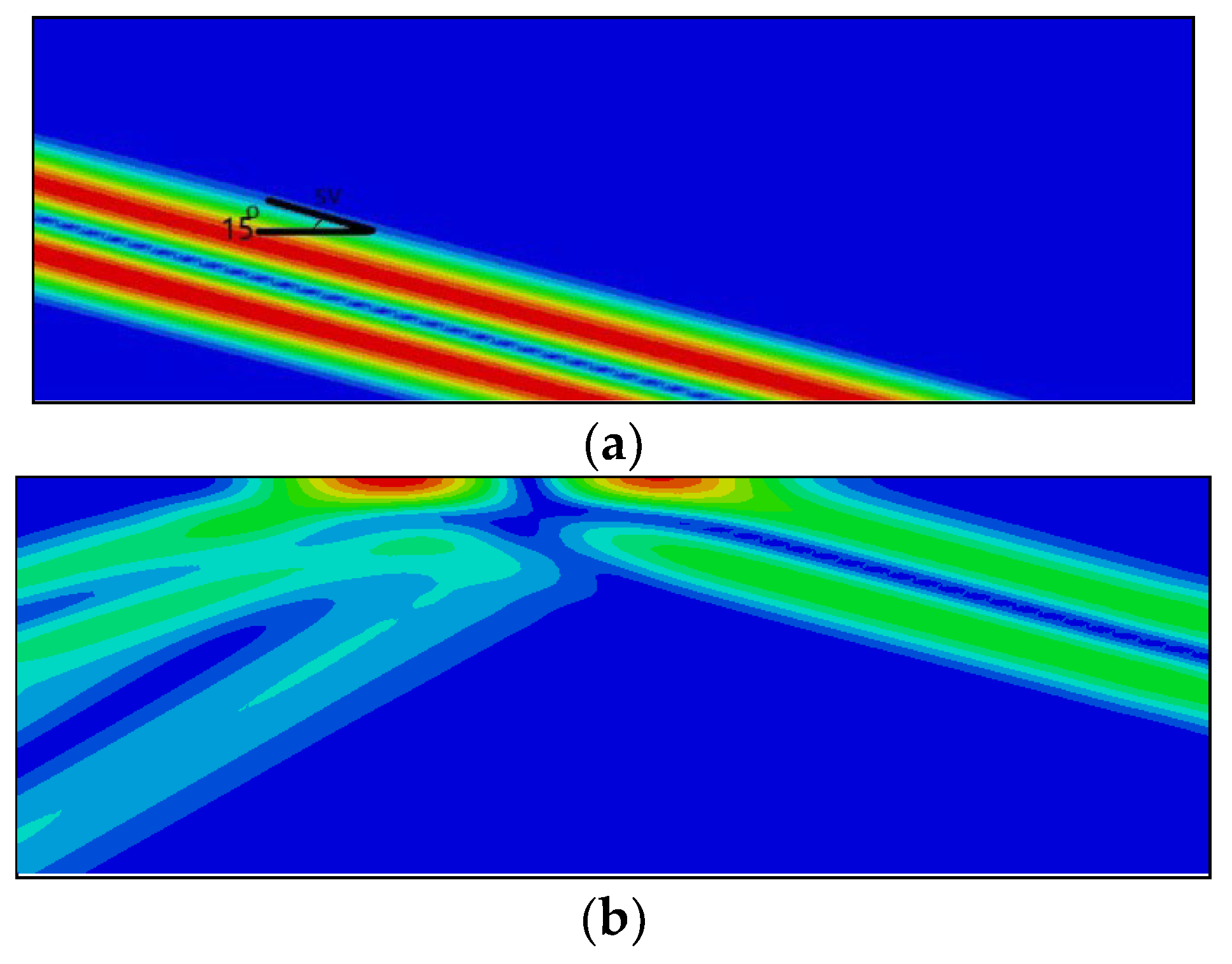
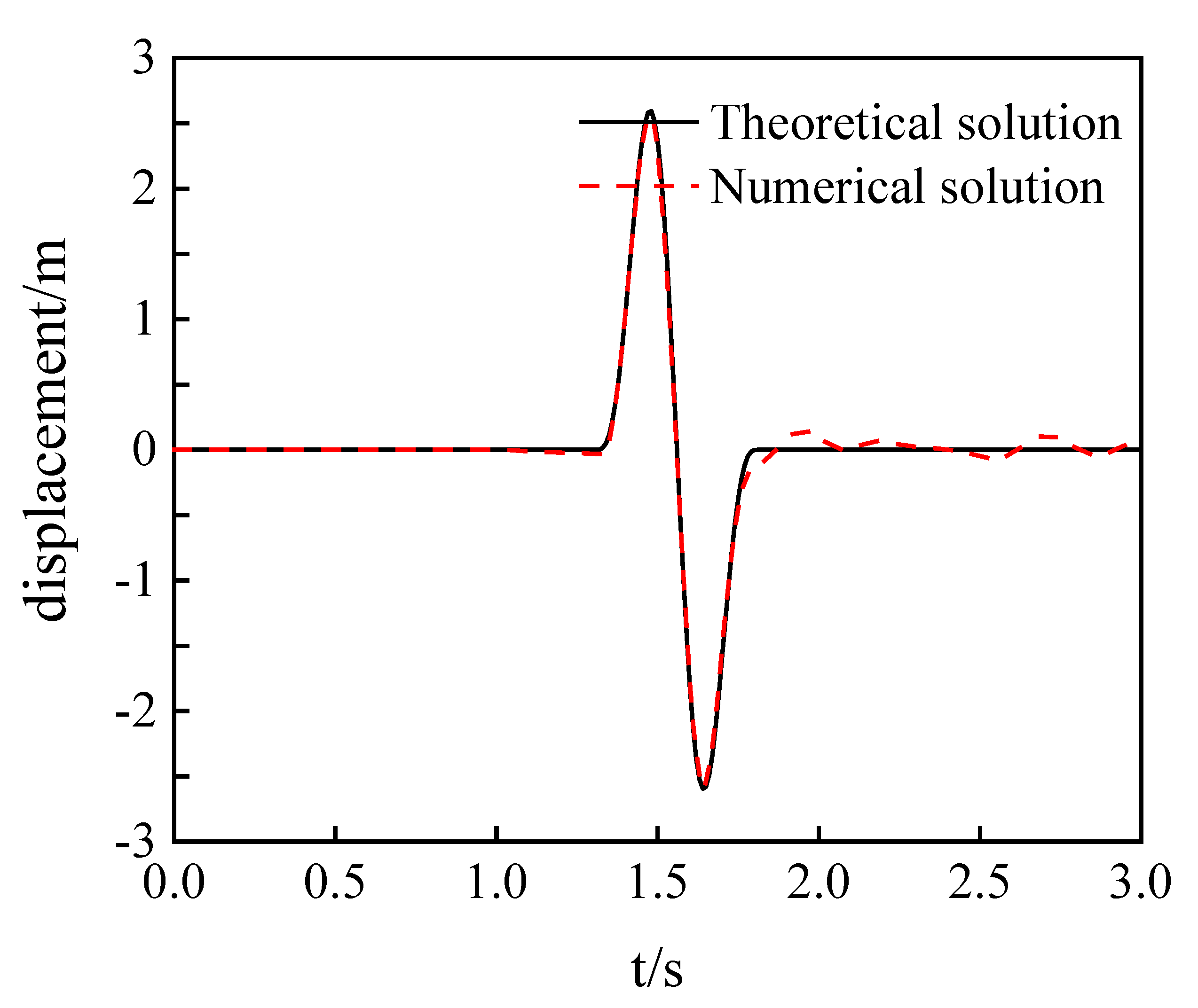
3. Seismic Input Verification

The elastic half-space model, as shown in Figure 2, was established in Abaqus. The model size was 1000 m × 500 m, with an SV wave on a 15° oblique incidence two-dimensional plane, the density of soil was $\rho$ = 2000 kg/m³, the elastic modulus was $E$ = 2 GPa, Poisson’s ratio $\mu$ was 0.3, and point A was used as the monitoring point for analysis. The analytical solution is used to verify the correctness of the numerical solution, so as to judge the correctness of the finite element model.

The time–history curve of the incident wave displacement is shown in Figure 3. We imported the node information file into MATLAB to calculate amplitude, load and spring file in the model in the form of nodal forces. The calculation results are shown in Figure 4.

The displacement field cloud diagram of SV wave at 15° oblique incidence is shown in Figure 4. The figure shows the oblique incidence of seismic waves, and the color represents the intensity of the superposition of seismic waves. It can be seen from Figure 5 that the numerical solution is basically the same as the theoretical solution, which verifies the correctness of the model.

4. Seismic Response Analysis of Raised Terrain

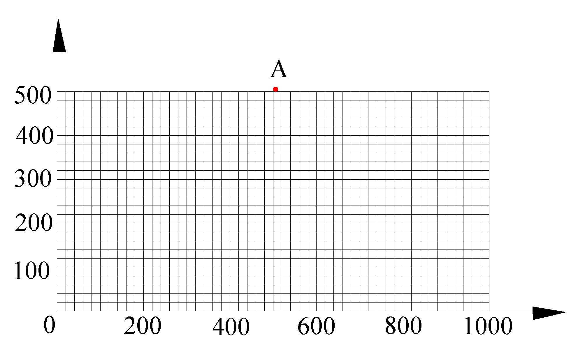
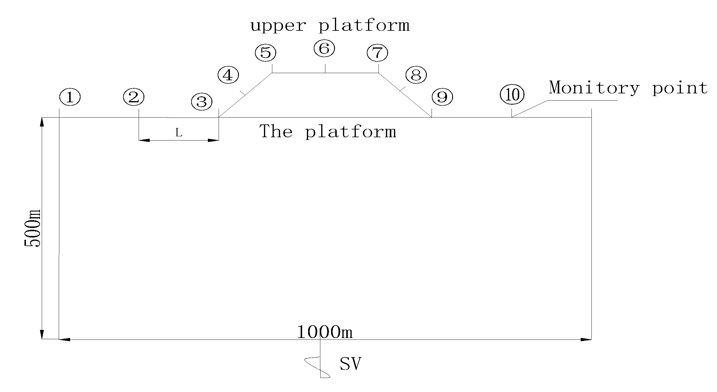
4.1. Establishing Finite Element Model

The finite element model of the raised terrain was 1000 m in length, 500 m in height, 100 m in platform height and 100 m in upper platform length. The corresponding monitoring points were arranged on the ground surface of the raised terrain, as shown in Figure 6. The modulus of elasticity: $E$ = 4.318 Gpa; Poisson’s ratio: $\mu$ = 0.25; density: $\rho$ = 1700 kg/m³, shear wave velocity: $c_s$ = 1000 m/s; and compression wave velocity: $c_p$ = 1732 m/s.

The angle of the foot of the terrain was measured as 30°, 45° and 60°, respectively. The seismic waves are obliquely incident from the left side of the terrain at 0°, 15° and 30°, respectively. The seismic waves are shown in Figure 7. The absolute value of the ratio between peak surface acceleration $A_{\max }$ and peak incident wave acceleration $A_{\max }{{}_{,}}_{input}$ is used as the ground motion amplification coefficient $\beta$, $\beta =\left|A_{\max }/A_{\max }{{}_{,}}_{input}\right|$. Figure 7 shows the seismic wave curve, and Figure 8 shows the Fourier spectrum of seismic wave.

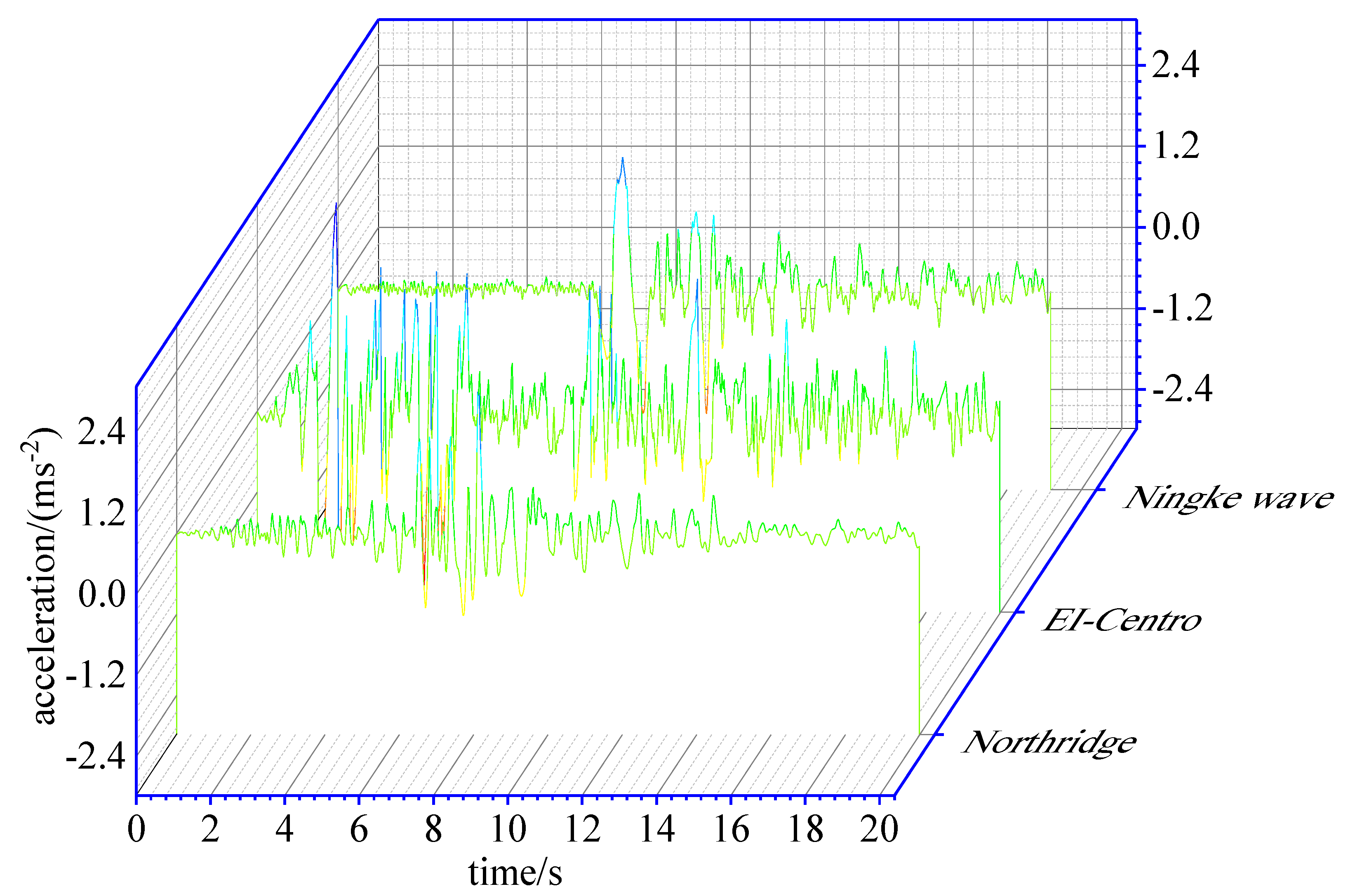
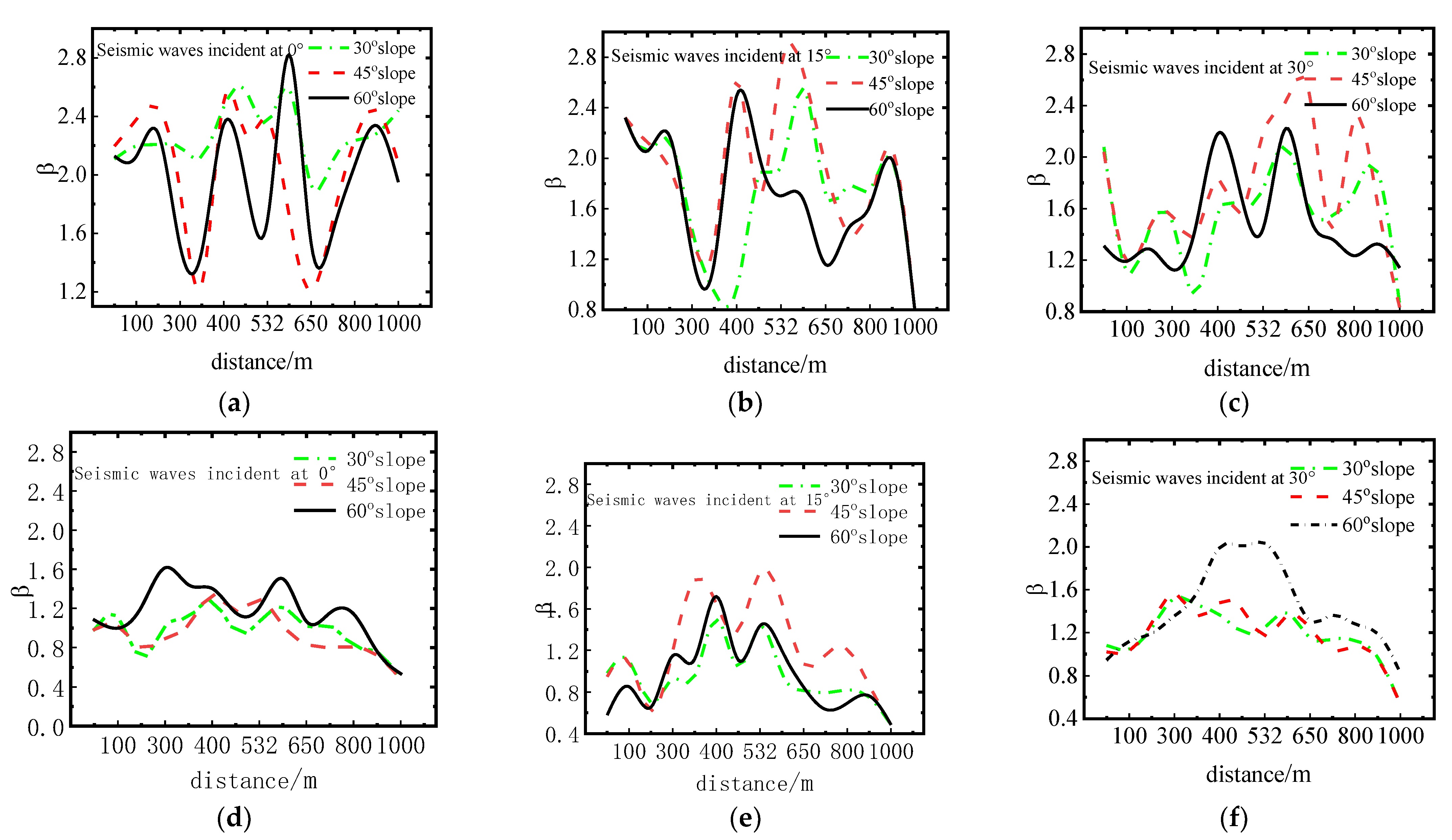
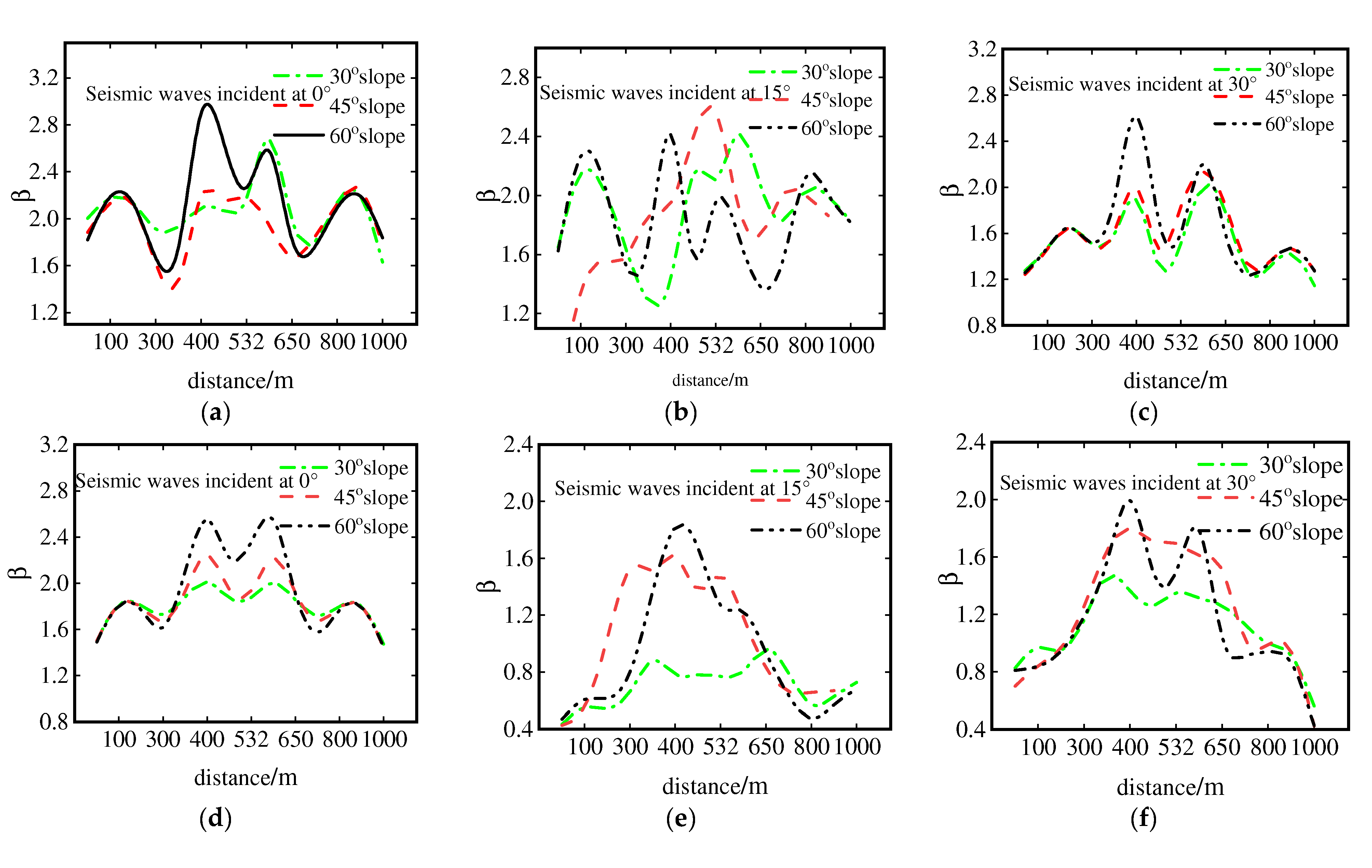
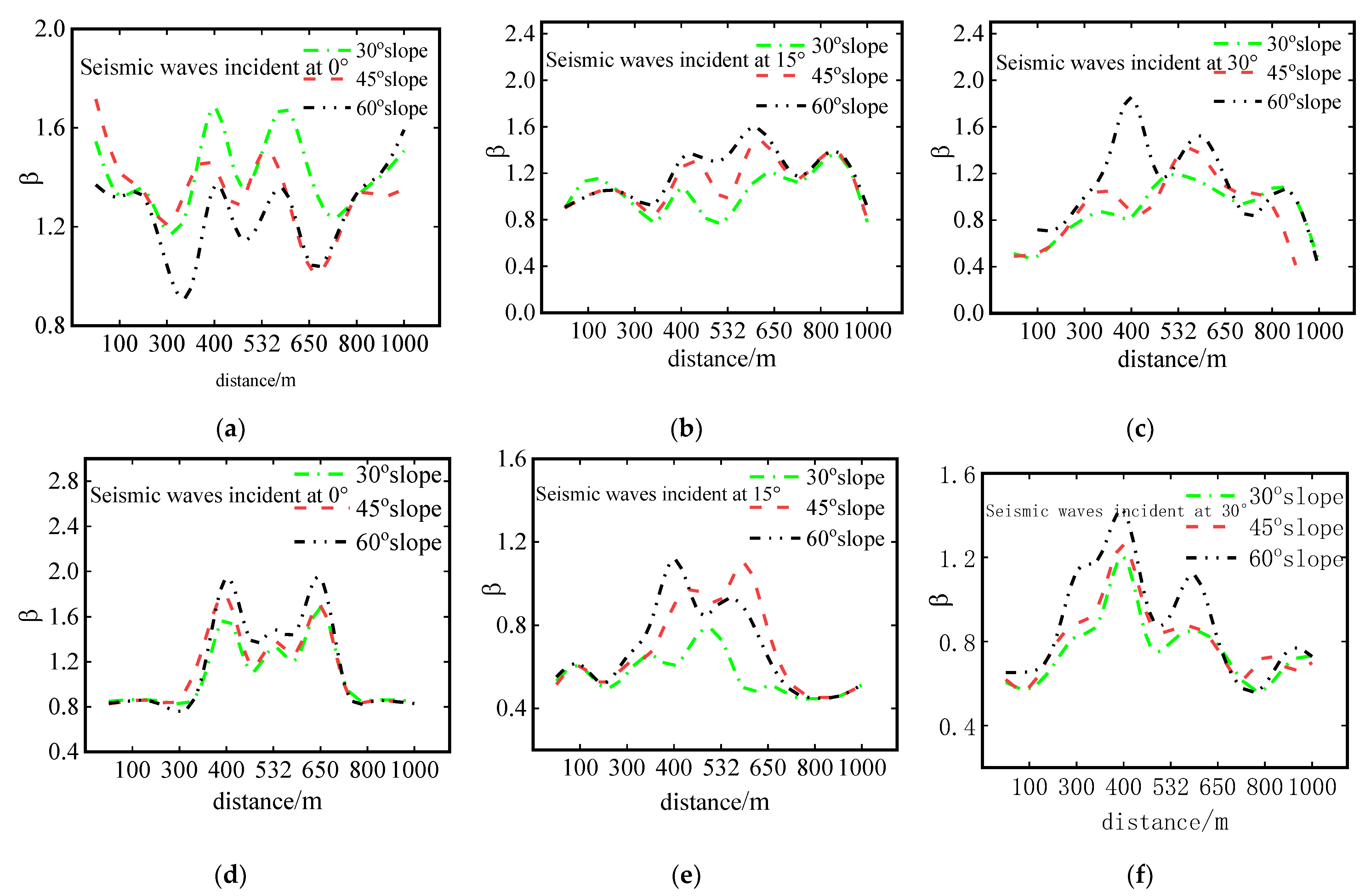
4.2. Response of Slope and Incident Angle to Ground Vibration of Raised Terrain

It can be seen from Figure 9, Figure 10 and Figure 11 that, when the incident angle is constant, the influence of the slope angle variation on the distribution of seismic amplification coefficient is analyzed. The incident angle is 15°, and for the x component, the left and right sides are not symmetric; the left-hand side is bigger than the right-hand side. The 45° slope is greater than the 30° slope. For the y component, the left and right sides are basically symmetrical, the 45° slope is larger than the 60° slope, which is larger than the 30° slope, and the amplification coefficient is less than two.

When the slope is fixed, the seismic amplification coefficient is affected by the incident angle of the seismic wave. When the slope is 60°, the left and right sides are basically symmetric. When a 0° incident occurs, the maximum value appears at monitoring point 7. For 15° incidence, the maximum value occurs at monitoring point 5. When the incidence is at 30°, the maximum value appears at monitoring point five.

It can be seen that the X-direction component is larger than the Y-direction component in the case of vertical incident seismic waves, thereby indicating that the ground motion amplification effect in the X-direction is more significant and earthquake destruction is greater. The oblique incidence of the SV wave will produce a reflected P wave and SV wave. Due to the complexity of the convex terrain, the complex reflection and scattering effect of seismic waves occur during the propagation process. The X-direction amplification coefficient is obviously asymmetric, and the Y-direction amplification coefficient on the left and right sides of the terrain has a certain symmetry.

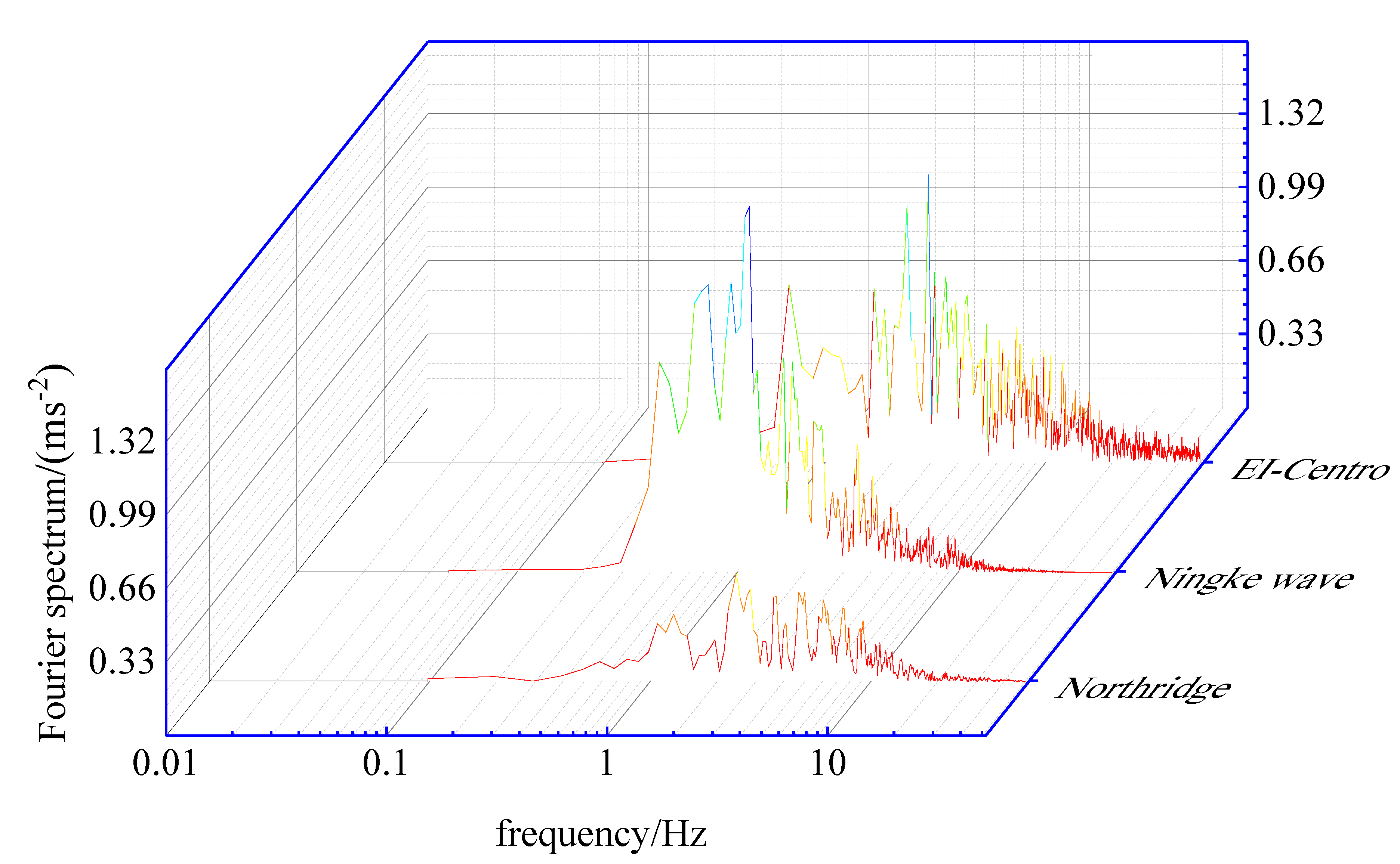
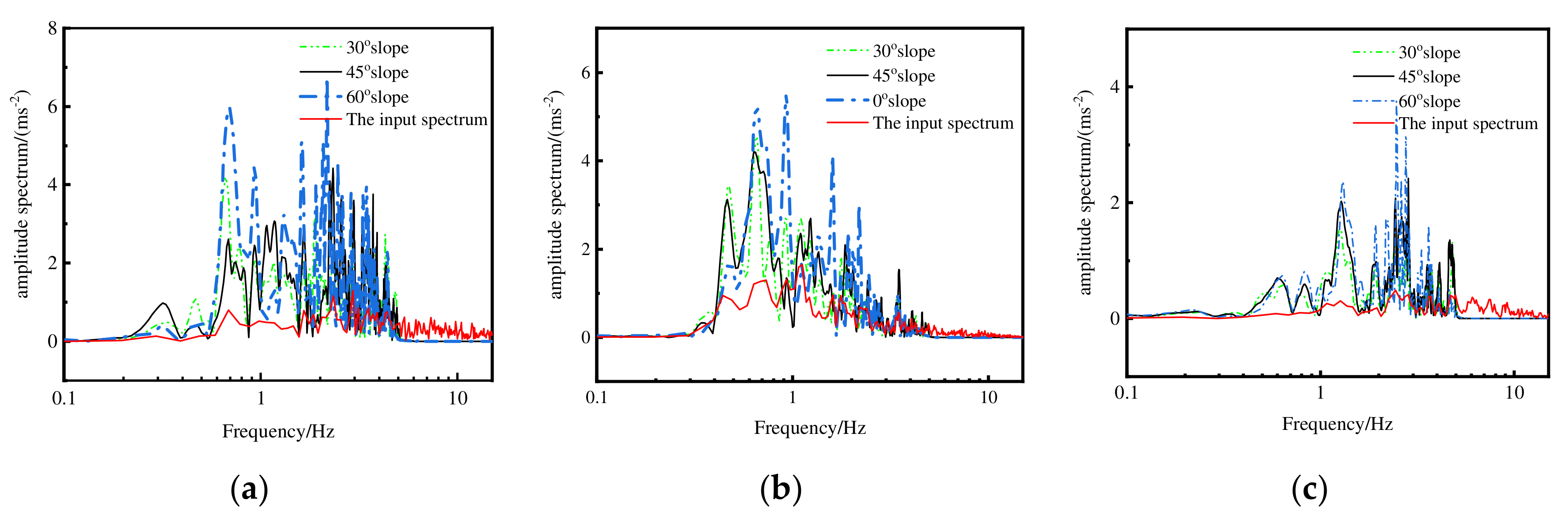
4.3. Effect of Topography on Fourier Spectrum of Ground Motion

The Fourier spectrum of the midpoint at the top of the slope is shown in Figure 12. Three kinds of seismic waves incident diagonally on the raised terrain with different slopes at different incident angles. It can be seen that the raised terrain has a significant amplification effect on the ground motion. The frequency is more obvious in the segment of 0.2~1 Hz. The overall change characteristic is that the Fourier spectrum value increases with the increase of the slope of the raised terrain. When the three seismic waves incident vertically on the raised terrain of different slopes, with frequencies ranging from 0.2 Hz to 1 Hz, and the Ningke wave incident, the Fourier general difference value is significant, and the Fourier spectrum value of the 30° slope in the low-frequency band is greater than that of the 45° slope. As shown in Figure 13, the influence of different incident angles on the Fourier spectrum of the raised terrain is analyzed under a certain slope. When the El Centro wave incident on the slope of 30°, the amplitude of the Fourier spectrum decreases with the increase of the incident angle in the low-frequency band, and the amplitude of the Fourier spectrum increases with the increase of the incident angle in the high-frequency band. The amplitude change rate is the largest. When the Ningke wave is oblique incident, the amplitude change in the input spectrum is basically the same as that of the seismic wave at 30°. The influence of low frequency and high frequency is the same as that of the El Centro wave. The amplitude of the Fourier spectrum is generally small when the Northridge wave is oblique incident. In short, the variation of the Fourier spectrum in the seismic site shows obvious differences under the coupling conditions of different incident angles and different frequencies.

5. Results

In this paper, the seismic response of raised terrain was selected, and the dynamic finite element method was used to simulate the ground motion amplification coefficient and Fourier spectrum variation of raised terrain with different angles of incidence by using a viscoelastic artificial boundary, and some laws were obtained.

(1)

When the slope is constant, the distribution of the oblique incident ground motion is much more complex than that of the vertical incident ground motion.

(2)

When the incident angle was constant, the amplification factor increased with the increase in the slope, and the left side of the site was larger than the right side. The amplification coefficients of the Y components were all less than two.

(3)

When the slope was fixed, with the increase of the incidence angle, the maximum value of the amplification coefficient shifted from the No. 7 monitoring point to the No. 5 monitoring point at the top of the slope, and the maximum value moved backward.

(4)

According to the Fourier spectrum curve diagram, the frequency was more obvious in the segment of 0.2~1 Hz, and the overall change was characterized by the larger Fourier spectrum value as the slope of the raised terrain increased.

(5)

When the El Centro wave was slanted into a 30° slope, the amplitude of the Fourier spectrum decreased with the increase of the incidence angle in the low-frequency band, and the amplitude of the Fourier spectrum increased with the increase of the incidence angle in the high-frequency band, and the change rate of the amplitude was the largest in the high-frequency band of 1–10 Hz.

References

1. Sánchez-Sesma, F.J.; Campillo, M. Topographic effects for incident p, sv and rayleigh waves. Tectonophysics 1993, 218, 113–125. [Google Scholar] [CrossRef]
2. Zhao, C.; Valliappan, S. Seismic wave scattering effects under different canyon topographic and geological conditions. Soil Dyn. Earthq. Eng. 1993, 12, 129–143. [Google Scholar] [CrossRef]
3. Lee, S.J.; Komatitsch, D.; Huang, B.S.; Tromp, J. Effects of Topography on Seismic-Wave Propagation:An Example from Northern Taiwan. Bull. Seismol. Soc. Am. 2009, 99, 314–325. [Google Scholar] [CrossRef] [Green Version]
4. Trifunac, M.D. Scattering of plane SH waves by a semi-cylindrical canyon. Earthq. Eng. Struct. Dyn. 1973, 1, 267–281. [Google Scholar] [CrossRef]
5. Tsaur, D.H. Scattering and focusing of SH waves by a lower semielliptic convex topography. Bull. Seismol. Soc. Am. 2011, 101, 2212–2219. [Google Scholar] [CrossRef]
6. Zhang, C.; Liu, Q.J.; Deng, P. Surface Motion of a Half-Space with a Semicylindrical Canyon under P, SV, and Rayleigh Waves. Bull. Seismol. Soc. Am. 2017, 107, 809–820. [Google Scholar] [CrossRef]
7. Ba, Z.; Wang, Y.; Liang, J.; Lee, V.W. Wave scattering of plane p, sv, and sh waves by a 3d alluvial basin in a multilayered half-space. Bull. Seismol. Soc. Am. 2020, 110, 576–595. [Google Scholar] [CrossRef]
8. Wong, H.L.; Trifunac, M.D. Scattering of plane SH waves by a semi-elliptical canyon. Earthq. Eng. Struct. Dyn. 1974, 3, 157–169. [Google Scholar] [CrossRef]
9. Ohtsuki, A.; Harumi, K. Effect of topography and subsurface inhomogeneities on seismic SV waves. Earthq. Eng. Struct. Dyn. 1983, 11, 441–462. [Google Scholar] [CrossRef]
10. Yuan, X.M.; Men, F.L. Scattering of plane SH waves by a semi-cylindrical hill. Earthq. Eng. Struct. Dyn. 1992, 21, 1091–1098. [Google Scholar] [CrossRef]
11. Tsaur, D.H.; Chang, K.H. Scattering and focusing of SH waves by a convex circular-arctopography. Geophys. J. Int. 2009, 177, 222–234. [Google Scholar] [CrossRef] [Green Version]
12. Fan, G.; Zhang, L.M.; Li, X.Y.; Fan, R.L.; Zhang, J.J. Dynamic response of rock slopes to oblique incident SV waves. Eng. Geol. 2018, 247, 94–103. [Google Scholar] [CrossRef]
13. Yin, C.; Li, W.H.; Zhao, C.G.; Kong, X.A. Impact of tensile strength and incident angles on a soil slope under earthquake SV-waves. Eng. Geol. 2019, 260, 105192. [Google Scholar] [CrossRef]
14. Deeks, A.J.; Randolph, M.F. Axisymmetric time-domain transmitting boundaries. J. Eng. Mech. 1994, 120, 25–42. [Google Scholar] [CrossRef]
15. Du, X.L.; Zhao, M.; Wang, J.T. A stress artificial boundary in FEA for near-field wave problem. Chin. J. Theor. Appl. Mech. 2006, 38, 49–56. [Google Scholar]
Figure 1. SV wave oblique incidence model.
Symmetry 14 02244 g001
Figure 2. This is a finite element model diagram (unit: m).
Symmetry 14 02244 g002
Figure 3. Time−history curve of incident SV wave displacement.
Symmetry 14 02244 g003
Figure 4. Displacement contours. (a) t = 0.8 s; (b) t = 1.6 s.
Symmetry 14 02244 g004
Figure 5. Comparison of the curves of theoretical and numerical displacement.
Symmetry 14 02244 g005
Figure 6. Layout of raised terrain and monitoring points.
Symmetry 14 02244 g006
Figure 7. Seismic wave acceleration.
Symmetry 14 02244 g007
Figure 8. Seismic Fourier spectrum.
Symmetry 14 02244 g008
Figure 9. El Centro wave with different angles of incidence and different slopes of raised terrain β . (a) x( θ = 0°); (b) x( θ = 15°); (c) x( θ = 30°); (d) y( θ = 0°); (e) y( θ = 15°); (f) y( θ = 30°).
Symmetry 14 02244 g009
Figure 10. Ningke wave with different angles of incidence and different slopes of raised terrain β . (a) x( θ = 0°); (b) x( θ = 15°); (c) x( θ = 30°); (d) y( θ = 0°); (e) y( θ = 15°); (f) y( θ = 30°).
Symmetry 14 02244 g010
Figure 11. Northridge wave with different angles of incidence and different slopes of raised terrain β . (a) x( θ = 0°); (b) x( θ = 15°); (c) x( θ = 30°); (d) y( θ = 0°); (e) y( θ = 15°); (f) y( θ = 30°).
Symmetry 14 02244 g011
Figure 12. Fourier spectrum of acceleration at the top of different slopes under 0° incident seismic wave. (a) El Centro waves; (b) Ningke waves; (c) Northridge waves.
Symmetry 14 02244 g012
Figure 13. Fourier spectrum of 30° acceleration at the top of the slope under different seismic waves and different incident angles. (a) El Centro waves; (b) Ningke waves; (c) Northridge waves.
Symmetry 14 02244 g013
Publisher’s Note: MDPI stays neutral with regard to jurisdictional claims in published maps and institutional affiliations.