Abstract
This paper discusses and compares several computed tomography (CT) algorithms capable of dealing with incomplete data. This type of problem has been proposed for a symmetrical grid and symmetrically distributed transmitters and receivers. The use of symmetry significantly speeds up the process of constructing a system of equations that is the foundation of all CT algebraic algorithms. Classic algebraic approaches are effective in incomplete data scenarios, but suffer from low convergence speed. For this reason, we propose the use of nature-inspired algorithms which are proven to be effective in many practical optimization problems from various domains. The efficacy of nature-inspired algorithms strongly depends on the number of parameters they maintain and reproduce, and this number is usually substantial in the case of CT applications. However, taking into account the specificity of the reconstructed object allows to reduce the number of parameters and effectively use heuristic algorithms in the field of CT. This paper compares the efficacy and suitability of three nature-inspired heuristic algorithms: Artificial BeeColony (ABC), Ant Colony Optimization (ACO), and Clonal Selection Algorithm (CSA) in the CT context, showing their advantages and weaknesses. The best algorithm is identified and some ideas of how the remaining methods could be improved so as to better solve CT tasks are presented.
1. Introduction
In the classic formulation of the computed tomography (CT) reconstruction problem, the interior of the examined object is reconstructed on the basis of its X-rays (projections) with a beam of penetrating radiation. Since each type of matter has a different ability to absorb radiation energy, appropriate algorithms recreate the interior of the examined object based on the energy loss of the emitted radiation beam. However, it is required that there are enough of these projections—many X-ray angles and many rays for each of these angles (see Kotelnikov’s theorem [1]).
In the classical approach (e.g., in medical tomography), modern tomographs are perfectly capable of recreating the examined interior. They find an image (also three-dimensional) with the desired accuracy (resolution) within a satisfactory time for doctors. Therefore, most of the work in this field concerns not the reproduction process itself, but rather a later stage—the analysis of this image or obtaining similar results with a lower dose of radiation (see, e.g., [2]).
Unfortunately, in many cases, we are not able to obtain projections that meet the desired criteria. An example of such a situation is the examination of a coal seam, in which there may be stone overgrowths that are not good for economic reasons, or pressurized gas tanks that are dangerous due to the threat to the life of the working crew. Such phenomena are really dangerous. In the largest Polish catastrophe caused by rock ejection (undetected compressed gas tank), which happened in the second half of the 20th century, nearly 20 miners were killed in the Nowa Ruda mine.
When examining the coal seam, the projections obtained are highly one-sided, because they can only be made between two opposite walls. Of course, there are methods of examining coal seams (e.g., drilling is performed), but these methods are uneconomical (and sometimes also dangerous), because mining must be suspended for the duration of the test.
Meeting the assumptions about the projection quality is a guarantee of the success of the process of recreating the interior of the tested object. However, the lack of its fulfillment does not exclude the final success. CT algorithms, which on the basis of the obtained projections return the image of the examined object, can be divided into two groups: analytical algorithms [3,4,5] and algebraic algorithms [6,7,8]. The conducted research has shown that the analytical algorithms cannot cope with a too-small number of scanning angles and therefore cannot be used in the problem of an incomplete dataset (see, e.g., [9]). For this reason, we focus on algebraic algorithms.
In the literature, it is difficult to find works on the use of heuristic algorithms in the CT problem (as presented in the following paper). The overwhelming majority of works using these algorithms in this task concern not the process of reproduction itself, but the analysis of an already obtained image [10,11,12]. The lack of works similar to this one results from the difficulty of using heuristic algorithms in the CT task. The classic approach would require too many parameters to be recreated. On the other hand, the conducted research and attempts to accelerate the playback (see, e.g., [9,13]) indicated the shortcomings of the classical approach. Therefore, we have leaned towards this line of research (see, for example, in [14], its first steps).
2. Algebraic Algorithms
For CT tasks, one can create any meshes, but in order to speed up the calculations, we use symmetry of engineeredmeshes and the symmetrical arrangement of transmitters and receivers of penetrating radiation. In the algebraic algorithms we are considering, it is assumed that the reproduced area can be divided into of identical squares (pixels), and this division is so dense that it can be assumed that the density distribution function has a constant value on each of these pixels. Thanks to this assumption, the energy loss of a single ray can be presented as the sum of the energy losses of this ray on individual pixels through which this ray passes. On the other hand, the energy loss on a single pixel is proportional to the length of this ray on that pixel (knowing the discretization density n and the equations of lines containing the rays, this length can be determined) and to the value of the function on this pixel (we have to recreate this value).
Considering all the rays in sequence, we obtain a system of linear equations of the form
where A is a matrix of the dimension coefficients (m is the number of projections made), X is a vector of unknown lengths N (each element is an unknown value of the function on successive pixels), and B is a vector of length m (each of its elements is the projection value, i.e., the total energy loss of the given ray).
Matrix A does not allow the use of classical methods of solving systems of linear equations. A large part of algebraic algorithms is based on Kaczmarz’s idea which is a special tag for the ART (algebraic reconstruction technique) algorithm, which is described below. In this algorithm, is i-th row of A, is the classically defined dot product in the space , is an i-th projection (in other words is an i-th element of B), , is the norm of the vector, in this case its length, and is the relaxation parameter. Algorithm 1 presents the ART procedure.
The ART algorithm runs as long as the stop condition is satisfied. Often the stop condition is a predetermined number of iterations (we assume that one iteration is going through all the lines of the A matrix, i.e., it is executing m projections). It is also assumed that the stop condition is a measure of the change of successive solutions—if the solutions change by less than a given amount, the algorithm ends its work. A combination of both conditions is also used.
| Algorithm 1: Algorithm ART. |
3. Task Formulation and Idea
In the case of an incomplete dataset, which is represented here by the coal seam survey, projections are obtained as shown in Figure 1, where orange points indicate radiation transmitters, red—receivers, brown arrows indicate ray paths and directions, and green rectangles—objects to be detected. We are dealing with the problem of an incomplete dataset because the obtained X-rays (projections) are “one-sided”. In medical tomography, projections are obtained from any angle (for a large number of such angles). In the examination of the coal seam, we can obtain data only on the basis of projections drawn between two opposite walls. Despite the fact that we can collect a lot of such data (e.g., as much as in medical tomography), their quality (not in the sense of the accuracy of measurements, but in the sense of the data on the interior of the examined object carried by these projections) will differ significantly from the information obtained in the tomography medical. As long as we assumed the symmetry of the grid and the distribution of transmitters and receivers of penetrating radiation, at this stage, due to the heterogeneity of the studied area, we obtain projection asymmetry, and in this case it leads to a solution.
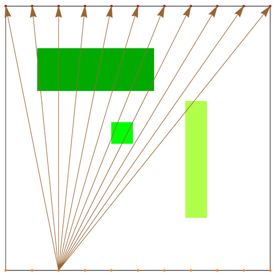
Figure 1.
Schematic model of CT rays’ projections in incomplete data processing mode.
The number of radiation sources and receivers determines the number of m rows of the A matrix of the (1) equation system, while the squared discretization density of the studied area determines the number of unknowns N. On the basis of the projections obtained in this way, the interior of the examined object should be recreated, i.e., the value of the density distribution function for each of the pixels should be found.
As we already mentioned, the analytical algorithms are sensitive to the quality of the projection (in this case, their number is not so important, but their unidirectional nature is), but they recreate the interior of the examined objects with a satisfactory accuracy. Although algebraic algorithms turned out to be useful in the problem of incomplete datasets, for stable, detected opaque elements, their problem is playback time—with increasing resolution (value of the N parameter), the number of rows of the equation system must increase (1), and this entails the need to perform a correspondingly larger number of iterations, which significantly extends the time (in the classic formulation of the CT reconstruction problem, a dozen or so iterations are often enough to obtain a satisfactory result, and in the presented problem of an incomplete dataset, the number of iterations can be counted in thousands).
Some attempts, most often effective, have been made to speed up the work of these algorithms. These methods include the selection of optimal values of reconstruction parameters, the introduction of chaotic algorithms, theoretical considerations on parallel computing—the introduction of block algorithms, or practical research related to the use of parallel computing in block algorithms [13,14].
These actions improved the recovery time; however, it seems that the mentioned time could be reduced much more. For this purpose, an innovative approach is used—heuristic algorithms are used to solve the CT task. Although naturally inspired algorithms were used in the problem of computed tomography [15,16,17,18,19,20], these approaches were of a different nature—these algorithms did not solve the (1) equation system, but had already reconstructed the image to improve its quality or cooperate with analytical algorithms.
In this work we compare the usefulness of three types of heuristic algorithms that have a very wide range of applications, e.g., for optimization of induction motors, continuous casting process research, to target recognition for low-altitude aircraft, to reduce noise pollution in rooms, airport traffic control, optimization of queries in a distributed database, aiding production planning, improving vehicle energy efficiency, analysis and segmentation of magnetic resonance images, prediction of wear symptoms of rubber products, solving the problem of nursing work planning, optimization of low microgrid configuration tensions, improvements in the system of granting access to data science resources, and even in viticulture and many others [21,22,23,24,25,26,27,28,29,30,31,32,33].
The first is the Artificial Bee Colony (ABC) algorithm. The ABC algorithm, similar to most nature-inspired algorithms, bases the method of its operation on the actual behavior of a certain organism. It was created on the basis of observations of bees looking for food. Bees are divided into three groups: randomly searching for food sources, searching for food in known sources, and observers waiting in the hive and making decisions about the choice of food source. The search for a solution in this algorithm is based on the information exchange system between different types of bees. The first to notice such behavior of bees was Frish, who at the end of the first half of the 20th century investigated and described this phenomenon [34]. Such behavior is based on the fact that when a new source of food is discovered (if, in the opinion of a given bee, this source is attractive), the bee informs other bees about the location of this source by appropriate movements (waggle dance). The initial bee moves in a straight line. Its direction is the angle between the sun and the food source, and its length is the distance to that source. Frish noticed that 75 ms of dancing (in a straight line) corresponded to 100 m off-road. The bee then returns in a semicircle (left or right) to its original position. The vibrations of the bee are an additional element of the dance. They determine the quality of the food. The actual bee dance can be seen (along with the description of the meaning of the dancing bee’s behavior), e.g., under the link [35]. An algorithm describing this behavior of bees was introduced by Karaboga in 2005 [36]. The equivalent of food sources are vectors from the considered space, the quality of food is interpreted by the value of the minimized functional, and the probability of selecting the source depends on the value of the functional. In general, it can be said that the area under investigation is searched twice—first the whole area is searched in general, and then the most promising areas in more detail.
Algorithm 2 presents the ABC procedure.
| Algorithm 2: Algorithm ABC. |
|
The second algorithm used in this work is the Ant Colony Optimization (ACO) algorithm. This is one of the best known swarm optimization algorithms. It was proposed by Dorigo in his doctoral dissertation [37], and later this method was developed; many sources mention Toksari [37] as the most important. This algorithm was created on the basis of observation of the behavior of ants searching for food and passing on knowledge about it to other ants. As in the case of bees, which conveyed information about their food source to other bees by means of appropriate dance, ants transmit information about the food place to other ants by means of scent traces (pheromone). Initially, the ants (represented by the appropriate vectors) run randomly across the field. The ant that comes back with food will take the shortest path and its pheromone trace will be the strongest, because it will have the least time to evaporate (the equivalent of the best ant is the vector for which the functional has the lowest value). The remaining ants do not have to choose the directions randomly, they make the decision to choose the path on the basis of pheromone traces left by the previous population, thus strengthening this trace (in the algorithm, the probability of choosing a direction corresponds to it). Of course, in order to not become stuck in the local minimum, the location of the ants must be modified (the values of the algorithm parameters correspond to this). Interesting applications and a slightly different approach to this algorithm can be found, among others, in the works [37,38].
Algorithm 3 presents the ACO procedure.
| Algorithm 3: Algorithm ACO. |
|
The third algorithm used in this work is the Clonal Selection Algorithm (CSA) [39]. This algorithm is based on the functioning of the mammalian immune system. The body produces antibodies to fight harmful foreign organisms (antigens). The effectiveness of combating them depends on the measure of how similar antibodies are to antigens. In the algorithm, this antigen is the solution sought, and the antibody is the solution obtained by the algorithm.
The algorithm shows that part of the population is cloned. The number of clones produced depends on their quality. All clones undergo a maturation process. Clones undergo random hypermutation. The clones are then validated. The best clones replace the previous ones from which they were created. The remaining elements of the population that were not cloned are replaced by new random elements.
Algorithm 4 presents the CSA procedure.
| Algorithm 4: Algorithm CSA. |
|
The idea of using heuristic algorithms in solving the CT task is as follows: in the coal seam, the density distribution is discrete and high-contrast; additionally, the resolution does not have to be very high—only tanks of considerable size are dangerous, although the possibility of reproducing elements was tested (with success) as the size of a single pixel.
For this reason, we can assume that in the area under consideration there may or may not be elements (we assume that there are no more than three) that have the shape of rectangles on which the density distribution function has a constant value. In turn, these rectangles can have at most a common segment.
Thanks to this approach, the cases in which the discussed method can be used are not limited, and the number of simultaneously recreated parameters (solution space dimension) is , where is the number of rectangles to be recreated. One rectangle is characterized by two coordinates of two opposite vertices and the value of the density distribution function on that rectangle.
The aim is to recreate the interior of the tested object based on the projection. The minimized functional here is:
where is real project, and is position for established objects.
4. Results
We start the experiments with the usability analysis of the ABC, ACO, and CSA algorithms in the case when in the searched area there is one rectangle , where the density distribution function takes the value 1. Initially, we run the programs for 400 pixels and 58 of sources and receivers of rays (for this resolution it is the optimal value of m). At this point, it is important to note a certain advantage of heuristic algorithms—they are not sensitive to increasing discretization. In classical algorithms, the recovery time significantly increases with the increase of the n parameter, in these algorithms only projections should be determined, and these only require, depending on the approach to this problem, either to multiply the matrix A and the vector X (this vector can be obtained very easily on the basis of the solution generated at a given stage), or by directly determining it (also on the same basis).
Figure 2 shows, for the ABC algorithm, the relationship between the number of iterations and the value of the objective functional (3) for different numbers of s bees.
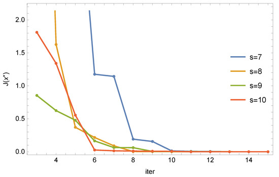
Figure 2.
ABC algorithm: relationship between the number of iterations and the value of the objective function for different numbers of bees.
Each of the parameter sets was run 10 times and the best one was selected from the series of results. As can be seen, after 10 iterations, the reproduction errors are very small, but for 10 bees, such results are obtained from 6 iterations. For example, for 6 iterations, for 10 bees, the rectangle R was recreated as follows: , the function assumed the value , and the objective function was . For 15 iterations and 10 bees, the values were equal to:
We now conduct similar tests for the ACO algorithm. In this algorithm there is an additional narrowing parameter , which we take depending on the number of iterations I according to the formula .
Figure 3 shows the relationship between the number of iterations and the value of the objective function (3) for different numbers of ants p for the ACO algorithm.
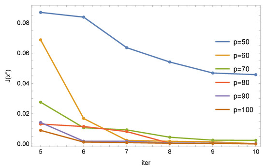
Figure 3.
ACO algorithm: relationship between the number of iterations and the value of the objective function for different numbers of ants.
Each of the parameter sets was run 10 times and the best one was selected from the series of results. As can be seen, this algorithm behaves correctly—the value of the objective function decreases with an increase in the number of iterations and with an increase in the number of ants. We can also notice that the algorithm responds better to increasing the number of ants. For example, for 6 iterations, for 100 ants, the R rectangle was recreated as follows: , function assumed the value , and the objective function was . For 10 iterations and for 100 bees, the values were equal to:
We now conduct similar tests for the CSA algorithm. This algorithm already has many more parameters, so it is not as intuitive as the previous two algorithms. After preliminary research and using previous experiences, we used the standard algorithm parameters. Figure 4 shows the dependence of the value of the objective function on the number of iterations for different sizes of the population.
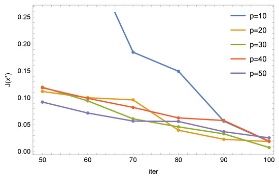
Figure 4.
CSA algorithm: relationship between the number of iterations and the value of the objective function for the size of the population.
Each of the parameter sets was run 10 times and the best one was selected from the series of results. As can be seen, this algorithm behaves correctly—the value of the objective function decreases with an increase in the number of iterations and with an increase in the size of the population. We can also notice that starting from a population of 20 individuals, the distribution of errors looks similar. For example, for 70 iterations, for a population of 70, the rectangle R was recreated as follows: , function assumed the value , and the objective function took a value of . For 100 iterations and for 100 positions, the values were equal to:
Figure 5, Figure 6 and Figure 7 graphically show the evolution of solutions obtained in ABC, ACO, and CSA algorithms, depending on the number of iterations. The dashed line is the exact solution. The restored value of the function on this rectangle is also given in the middle of the approximate solution (the exact value is 1).
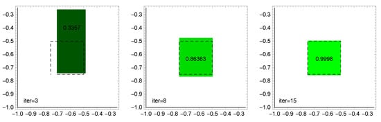
Figure 5.
ABC algorithm: evolution of solutions depending on the number of iterations (8 bees).
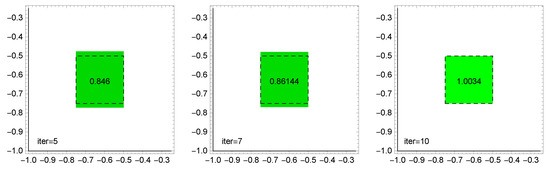
Figure 6.
ACO algorithm: evolution of solutions depending on the number of iterations (100 ants).
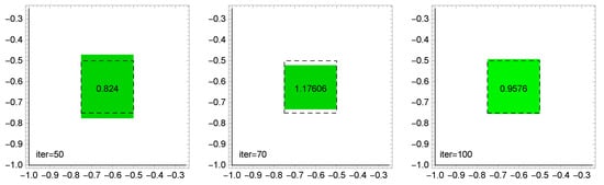
Figure 7.
CSA algorithm: evolution of solutions depending on the number of iterations (population size 100).
In subsequent tests, we increased the number of rectangles by one. This time we have two rectangles, and , where the density distribution function takes values equal to 1 and 2, respectively.
The program is structured in such a way that if the objective function does not reach the satisfactory value while searching for one rectangle, it restarts, searching for two rectangles (likewise, it may increase the number of rectangles to three). In the ABC algorithm, it turned out that it copes with this problem. For example, for 9 bees and 15 iterations, the program returned the following recreations:
Unfortunately, the ACO and CSA algorithms are not able to recreate two (and therefore also three) rectangles. This is probably caused by the way of representing rectangles and solution vectors as well as the specificity of algorithms that use the measure of similarity between successive solutions. As a result, good solutions may be interpreted as seemingly different. There are already some ideas on how to overcome this problem, but this requires a lot of additional and time-consuming research to be carried out in the future.
Since the main aim of the research carried out here was to shorten the recovery time, we now compare the working times of reconstructing one rectangle for the algorithms under consideration. In Table 1, Table 2 and Table 3, the working times of the algorithms for different sizes of the population and the number of iterations are collected. After selecting the best pairs of these parameters, Table 4 presents a statement for the best of these algorithms: the value of the goal function , the average of the goal function values, the standard deviation of these results, and the average time needed to obtain these plays.

Table 1.
ABC algorithm: time t (ms) to obtain a solution and maximum coefficient of variation depending on the size of the p population and the number of iterations I.
Table 2.
ACO algorithm: time t (ms) to obtain a solution and maximum coefficient of variation depending on the size of the p population and the number of iterations I.
Table 3.
CSA algorithm: time (ms) to obtain a solution and maximum coefficient of variation depending on the size of the p population and the number of iterations I.
Table 4.
ABC algorithm: value of the goal function to solve the best , the average of the value of the goal function , the standard deviation of these results , and the average time to obtain them, t, for 8, 9, and 10 runs.
As a measure of algorithm convergence, we use the maximum coefficient of variation, the size of which represents the repeatability of the obtained results in many samples. Assuming that , for are n independent solutions of the same problem obtained in n independent trials, the maximum coefficient of variation is given by the formula:
where is the average restore value of i-th parameter, and d is the number of parameters restored.
Comparing the obtained results, it can be easily noticed that even the most time-consuming set of parameters in the ABC algorithm generates a time shorter than the least time-consuming pair of parameters in the other algorithms. In addition, and in the ABC algorithm are definitely exaggerated values, and in the other algorithms, the set of parameter pairs for the shortest times is too small. In conjunction with the fact that the ABC algorithm can also deal with a larger number of reconstructed rectangles, it becomes the clear winner among the algorithms compared here. In addition, it should be mentioned that the time needed to recreate the interior of the object is incomparably shorter than the time needed by the classic CT algorithms (in the case of an incomplete dataset).
As can be seen, the ABC algorithm is not only effective but is also stable. The mean value of the objective function is as low as and the standard deviation is . The average time also does not differ from the corresponding (see Table 1) previously obtained time.
Finally, underlining the usefulness of the ABC algorithm, in Figure 8 we show how it recreates the three rectangles shown in Figure 1:
and the density distribution function on these rectangles is equal to 1, 2, and , respectively.
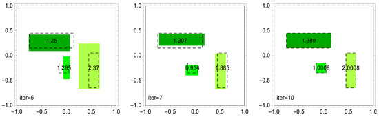
Figure 8.
ABC algorithm: evolution of solutions depending on the number of iterations (10 bees).
5. Conclusions
The tested algorithms turned out to be useful in solving the task of computed tomography with an incomplete dataset. All of the considered algorithms are characterized by significantly shorter recovery times than the classic CT algorithms with an incomplete dataset. Among the heuristic algorithms discussed in this paper, the ABC algorithm turned out to be the best in many respects. It had the best play times, was the most intuitive to use (no extra parameters), and was good at handling multiple rectangles.
A further direction of research will be the modification of approaches to the ACO and CSA algorithms, so that they also correctly reproduce the tested objects with more than one rectangle. The next step will be to modify the idea by recreating other types of objects.
Author Contributions
Conceptualization, A.Z.; Formal analysis, M.P., A.Z. and M.W.; Project administration, M.P.; Software, A.Z.; Visualization, M.P.; Writing—original draft, M.W.; Writing—review & editing, M.W. All authors have read and agreed to the published version of the manuscript.
Funding
Authors would like to acknowledge contribution to this research from the Rector of the Silesian University of Technology, Gliwice, Poland under pro-quality grant no. 09/010/RGJ22/0066 and no. 09/010/RGJ22/0068.
Institutional Review Board Statement
Not applicable.
Informed Consent Statement
Not applicable.
Data Availability Statement
Not applicable.
Conflicts of Interest
The authors declare no conflict of interest.
References
- Natterer, F. The Mathematics of Computerized Tomography; Wiley: Hoboken, NJ, USA, 1986. [Google Scholar]
- Malczewski, K. Image Resolution Enhancement of Highly Compressively Sensed CT/PET Signals. Algorithms 2020, 13, 129. [Google Scholar] [CrossRef]
- Averbuch, A.; Shkolnisky, Y. 3D Fourier Based Discrete Radon Transform. Appl. Comput. Harmon. Anal. 2003, 15, 33–69. [Google Scholar] [CrossRef]
- Lewitt, R. Reconstruction algorithms: Transform methods. Proc. IEEE 1983, 71, 390–408. [Google Scholar] [CrossRef]
- Waldén, J. Analysis of direct Fourier method for computed tomography. IEEE Trans. Med. Imaging 2000, 19, 211–222. [Google Scholar] [CrossRef]
- Andersen, A.H.; Kak, A.C. Algebraic Reconstruction in CT from limited views. Simultaneous algebraic reconstruction technique (SART): A superior implementation of the ART algorithm. Ultrason. Imaging 1984, 6, 81–94. [Google Scholar] [CrossRef]
- Gordon, R.; Bender, R.; Herman, G. Algebraic reconstruction techniques (ART) for three-dimensional electron microscopy and X-ray photography. J. Theor. Biol. 1970, 29, 471–481. [Google Scholar] [CrossRef]
- Guan, H.; Gordon, R. Computed tomography using algebraic reconstruction techniques with different projection access schemes: A comparison study under practical situation. J. Theor. Biol. 1996, 41, 1727–1743. [Google Scholar] [CrossRef] [PubMed]
- Hetmaniok, E.; Ludew, J.; Pleszczyński, M. Examination of stability of the computer tomography algorithms in case of the incomplete information for the objects with non-transparent elements. In Selected Problems on Experimental Mathematics; Silesian University of Technology Press: Gliwice, Poland, 2017; pp. 39–59. [Google Scholar]
- Woźniak, M.; Siłka, J.; Wieczorek, M. Deep neural network correlation learning mechanism for CT brain tumor detection. Neural. Comput. Appl. 2021, 1–16. [Google Scholar] [CrossRef]
- Sage, A.; Badura, P. Intracranial Hemorrhage Detection in Head CT Using Double-Branch Convolutional Neural Network, Support Vector Machine, and Random Forest. Appl. Sci. 2020, 10, 7577. [Google Scholar] [CrossRef]
- Khan, M.A.; Alhaisoni, M.; Tariq, U.; Hussain, N.; Majid, A.; Damaševičius, R.; Maskeliūnas, R. COVID-19 Case Recognition from Chest CT Images by Deep Learning, Entropy-Controlled Firefly Optimization, and Parallel Feature Fusion. Sensors 2021, 21, 7286. [Google Scholar] [CrossRef]
- Pleszczyński, M. Implementation of the computer tomography parallel algorithms with the incomplete set of data. PeerJ Comput. Sci. 2021, 7, e339. [Google Scholar] [CrossRef] [PubMed]
- Pleszczyński, M.; Zielonka, A.; Połap, D.; Woźniak, M.; Mańdziuk, J. Polar Bear Optimization for Industrial Computed Tomography with Incomplete Data. In Proceedings of the 2021 IEEE Congress on Evolutionary Computation (CEC), Kraków, Poland, 28 June–1 July 2021; pp. 681–687. [Google Scholar]
- Ashour, A.S.; Samanta, S.; Dye, N.; Kausar, N.; Abdessalemkaraa, W.B.; Hassanien, A.E. Computed Tomography Image Enhancement Using Cuckoo Search: A Log Transform Based Approach. J. Signal Inf. Process. 2017, 6, 244–257. [Google Scholar] [CrossRef]
- Dey, N.; Ashour, A.S. Meta-Heuristic Algorithms in Medical Image Segmentation: A Review. IGI Glob. Adv. Appl. Metaheuristic 2018, 6, 185–203. [Google Scholar]
- Lohvithee, M.; Sun, W.; Chretien, S.; Soleimani, M. Ant Colony-Based Hyperparameter Optimisation in Total Variation Reconstruction in X-ray Computed Tomography. Sensors 2021, 21, 591. [Google Scholar] [CrossRef] [PubMed]
- Chen, Y.-C.; Wang, H.-C.; Su, T.-J. Particle Swarm Optimization for Image Noise Cancellation. In Proceedings of the First International Conference on Innovative Computing, Information and Control—Volume I (ICICIC’06), Beijing, China, 30 August–1 September 2006; pp. 587–590. [Google Scholar]
- Würfl, T.; Ghesu, F.C.; Christlein, V.; Maier, A. Deep Learning Computed Tomography. In Proceedings of the Medical Image Computing and Computer-Assisted Intervention—MICCAI 2016, Athens, Greece, 17–21 October 2016; pp. 432–440. [Google Scholar]
- Shahamatnia, E.; Ebadzadeh, M.M. Application of particle swarm optimization and snake model hybrid on medical imaging. In Proceedings of the 2011 IEEE Third International Workshop On Computational Intelligence in Medical Imaging, Paris, France, 11–15 April 2011; pp. 1–8. [Google Scholar]
- Ang, L.M.; Seng, K.P.; Ge, F.L. Natural Inspired Intelligent Visual Computing and Its Application to Viticulture. Sensors 2017, 17, 1186. [Google Scholar] [CrossRef] [PubMed]
- Campelo, F.; Guimaraes, F.G.; Igarashi, H.; Ramirez, J.A. A clonal selection algorithm for optimization in electromagnetics. IEEE Trans. Magn. 2005, 41, 1736–1739. [Google Scholar] [CrossRef]
- Donati, A.V.; Krause, J.; Thiel, C.; White, B.; Hill, N. An Ant Colony Algorithm for Improving Energy Efficiency of Road Vehicles. Energies 2020, 13, 2850. [Google Scholar] [CrossRef]
- Guo, X.; Yuan, X.; Hou, G.; Zhang, Z.; Liu, G. Natural Aging Life Prediction of Rubber Products Using Artificial Bee Colony Algorithm to Identify Acceleration Factor. Polymers 2022, 14, 3439. [Google Scholar] [CrossRef] [PubMed]
- Kubicek, J.; Varysova, A.; Cerny, M.; Hancarova, K.; Oczka, D.; Augustynek, M.; Penhaker, M.; Prokop, O.; Scurek, R. Performance and Robustness of Regional Image Segmentation Driven by Selected Evolutionary and Genetic Algorithms: Study on MR Articular Cartilage Images. Sensors 2022, 22, 6335. [Google Scholar] [CrossRef]
- Muniyan, R.; Ramalingam, R.; Alshamrani, S.S.; Gangodkar, D.; Dumka, A.; Singh, R.; Gehlot, A.; Rashid, M. Artificial Bee Colony Algorithm with Nelder–Mead Method to Solve Nurse Scheduling Problem. Mathematics 2022, 10, 2576. [Google Scholar] [CrossRef]
- Mohsin, S.A.; Younes, A.; Darwish, S.M. Dynamic Cost Ant Colony Algorithm to Optimize Query for Distributed Database Based on Quantum-Inspired Approach. Symmetry 2021, 13, 70. [Google Scholar] [CrossRef]
- Paprocka, I.; Krenczyk, D.; Burduk, A. The Method of Production Scheduling with Uncertainties Using the Ants Colony Optimisation. Appl. Sci. 2021, 11, 171. [Google Scholar] [CrossRef]
- Rokicki, Ł. Optimization of the Configuration and Operating States of Hybrid AC/DC Low Voltage Microgrid Using a Clonal Selection Algorithm with a Modified Hypermutation Operator. Energies 2021, 14, 6351. [Google Scholar] [CrossRef]
- Tao, W.; Ma, Y.; Xiao, S.; Cheng, Q.; Wang, Y.; Chen, Z. An Active Indoor Noise Control System Based on CS Algorithm. Appl. Sci. 2022, 12, 9253. [Google Scholar] [CrossRef]
- Xu, B.; Ma, W.; Ke, H.; Yang, W.; Zhang, H. An Efficient Ant Colony Algorithm Based on Rank 2 Matrix Approximation Method for Aircraft Arrival/Departure Scheduling Problem. Processes 2022, 10, 1825. [Google Scholar] [CrossRef]
- Xu, C.; Duan, H. Artificial bee colony (ABC) optimized edge potential function (EPF) approach to target recognition for low-altitude aircraft. Pattern Recognit. Lett. 2010, 31, 1759–1772. [Google Scholar] [CrossRef]
- Zamri, N.E.; Mansor, M.A.; Mohd Kasihmuddin, M.S.; Alway, A.; Mohd Jamaludin, S.Z.; Alzaeemi, S.A. Amazon Employees Resources Access Data Extraction via Clonal Selection Algorithm and Logic Mining Approach. Entropy 2020, 22, 596. [Google Scholar] [CrossRef]
- von Frish, K. Die tänze der bienen. Österr. Zool. Z. 1948, 1, 1–48. [Google Scholar]
- Available online: https://www.youtube.com/watch?v=1MX2WN-7Xzc (accessed on 24 September 2022).
- Karaboga, D. An Idea Based on Honey Bee Swarm for Numerical Optimization; Technical Report—TR06; Computer Engineering Department, Engineering Faculty, Erciyes University: Kayseri, Turkey, 2005. [Google Scholar]
- Toksari, M.D. Ant colony optimization for finding the global minimum. Appl. Math. Comput. 2006, 176, 308–316. [Google Scholar] [CrossRef]
- Socha, K.; Dorigo, M. Ant colony optimization for continuous domains. Eur. J. Oper. Res. 2008, 185, 1155–1173. [Google Scholar] [CrossRef]
- de Castro, L.N.; Von Zuben, F.J. Learning and optimization using the clonal selection principle. IEEE Trans. Evol. Comput. 2002, 6, 239–251. [Google Scholar] [CrossRef]


Publisher’s Note: MDPI stays neutral with regard to jurisdictional claims in published maps and institutional affiliations. |
© 2022 by the authors. Licensee MDPI, Basel, Switzerland. This article is an open access article distributed under the terms and conditions of the Creative Commons Attribution (CC BY) license (https://creativecommons.org/licenses/by/4.0/).