A Method Converting Multi-Properties Objective Reachability Problems to Multi-Objective Sets Reachability Problems over FKS

Abstract

In this paper, we focus on the symmetrical relationship between multi-properties objective reachability problems and multi-objective sets reachability problems over FKS based on Zadeh logic. First, we give the formal definitions of those two problems. Then, we study their relationships and find that a multi-properties objective reachability problem and a special case of multi-objective sets reachability problems have symmetry. Finally, we give a polynomial time algorithm based on this symmetry to convert a multi-properties objective reachability problem to a multi-objective sets reachability problem. In addition, an illustrative example is listed to express some possible application methods based on our work.

1. Introduction

Fuzzy set theory is widely used in artificial intelligence [1,2,3,4], which pays more attention to the true value of the properties, a kind of uncertainty caused by unclear concept extension [5,6,7]. For example, we can not give an accurate definition and boundary between baldness and non-baldness. Planning algorithms [8,9,10,11,12] aim to find strategies which perform well (or even optimally) for a given objective. With the development of fuzzy theory in application, it will become more and more common that the problems related to the combination of planning algorithms and fuzzy theory [13,14,15,16,17,18,19]—for instance, whether there is a treatment during which the patient remains relaxed and his blood pressure was not high, where relaxed and not high are two fuzzy concepts, or this problem, whether there is a process during which a student learns mathematics, philosophy, biology, and chemistry well under the curriculum of one semester, where well is also a fuzzy concept. From the above examples, we can see that there are two classes of multi-problems: one is an objective with multi-properties, and another is a property but with multi-objectives. We describe the multi-properties objective reachability problem and multi-objective sets reachability problem, respectively. These two problems are also common, and there is some related work about those two problems listed in the following two paragraphs.

For the multi-properties objective reachability problem, there has been lots of related research work [20,21,22]. Hartmanns et al. [20] use Markov decision processes as the model and use sequential value iteration studying multi-cost bounded trade-off in Markov decision processes. Quatmann et al. [21] use Markov automata as the model, convert multiple properties objective problems in Markov automata to problems in Markov decision processes and problems in digitization Markov automata, and investigate algorithms.

For the multi-objective sets reachability problem, there also has been lots of related research work [9,23,24,25,26,27]. Chatterjee et al. [9] use graphs, Markov decision processes, and games on graphs as the models, investigate the sequential target reachability problems, and give polynomial algorithms to solve them. Li et al. [24,26] use a multi-valued transition system as the model, use trace sets expressing paths with specific properties and study some problems related to reachability by automata theory.

However, the above studies are all based on probability or multi-value and could be not able to describe and solve the examples in the paragraph above, and there are no formal definitions of these two problems in fuzzy scenarios. In other words, the formal definitions of those two problems in fuzzy scenarios are ambiguous, and the relationship and symmetry between them are the same. Zadeh fuzzy logic is a special fuzzy logic, based on which we maybe find a method to solve the problems of fuzzy scenarios. At the same time, there have been many studies on Zadeh fuzzy theory [19,28,29,30], which are also good theoretical bases for us. Therefore, we first give the formal definitions of those two problems in Zadeh fuzzy scenarios, and then study the relationship between them. In addition, we propose some possible application methods based on their relationship.

The goals of this paper are to formally describe two classes of multi-problems in Zadeh fuzzy logic which are gradually emerging due to the application and development of fuzzy theory in artificial intelligence, and to explain the relationships between the two problems, which means that we could solve one problem to solve another or use the solution of one problem in the process of solving another problem. The main contributions of this paper are as follows:

(1)

The formal definition of the multi-properties objective reachability problem and multi-objective sets reachability problem over FKS based on Zadeh logic is proposed, which can be used to describe some multi-requirements of fuzzy systems;

(2)

The symmetry between a multi-properties objective reachability problem and a special case of multi-objective sets reachability problems is studied, which is also a method of transforming a multi-properties objective reachability problem over FKS based on Zadeh logic to a multi-objective sets reachability problem. In this way, we can investigate the relationship between properties by studying the relationship between sets. At the same time, this also establishes a link between the two multi-problems in Zadeh fuzzy scenarios;

(3)

A polynomial time conversion algorithm is proposed and analysed, and an illustrative example is listed, which means that our method and algorithm are applicable.

Structure of the paper. The rest of the paper is organized as follows: In Section 2, the basic theoretical knowledge of fuzzy mathematics and fuzzy Kripke structures are given. In Section 3, we introduce the formal definitions of the multi-properties objective reachability problem and the multi-objective sets reachability problem over FKS based on Zadeh logic, and propose a method from which we can transmit a multi-properties objective reachability problem over FKS based on Zadeh logic to a multi-objective sets reachability problem. The polynomial time conversion algorithm is also proposed in Section 3. In Section 4, an illustrative example is listed to show the details of our method and algorithm, and some possible application methods of combining properties and objective sets. Section 5 summarizes this paper and gives the future research directions.

2. Preliminaries

Fuzzy set is a mathematical concept proposed by Zadeh in 1965. Fuzziness is due to the uncertainty caused by the breaking of the law of the excluded middle, i.e., the transition from one state to another is a continuous process when quantitative changes accumulate and eventually result in a qualitative change, which makes there be no clear boundary between “stability” and “instability”. Let us first review some notions of fuzzy sets and fuzzy logics. For a detailed introduction to the notions, the reader may refer to [5,6,7,31].

Let X be a universal set. A fuzzy set A of X is a function which associates each element in X a value in the interval $[0,1]$, i.e., $A:X⟶[0,1]$. For $x\in X$, $A\left(x\right)$ is the membership of x in the fuzzy set A. $\mathcal{F}\left(X\right)$ represents the set of all fuzzy sets in X, i.e., $\mathcal{F}\left(X\right)=\left\{A\right|A:X⟶[0,1]\}$. For $A,B\in \mathcal{F}\left(X\right)$, we use $A\cup B$ and $A\cap B$ to represent the union and intersection of A and B, respectively, where $(A\cup B)\left(x\right)=A\left(x\right)\vee B\left(x\right)=max\left\{A\right(x),B(x\left)\right\}$ and $(A\cap B)\left(x\right)=A\left(x\right)\wedge B\left(x\right)=min\left\{A\right(x),B(x\left)\right\}$. We can easily know that the union and intersection have idempotent law, commutative law, associative law, absorption law, and distributive law, which are important in our work.

Next, we recall some notations and definitions concerning FKSs. For a detailed introduction to the notions, the reader may refer to [28].

A fuzzy Kripke structure over $AP$ is a tuple $\mathcal{K}=(S,P,s_0,L)$, where

• S is a countable, non-empty set of states;
• P is a mapping from $S\times S$ to $[0,1]$, also known as fuzzy transition function;
• $s_0\in S$ is the initial state;
• L is a labeling function $L:S⟶\mathcal{F}\left(AP\right)$ that assigns a truth value in $[0,1]$ to an atomic proposition in a state.

An FKS is said to be finite if both S and $AP$ are finite.

A state sequence $s_0{s}_1{s}_2\cdots \in S^{\omega }$ over $\mathcal{K}$ is an infinite path from $s_0$ iff $P(s_{i-1},s_i)>0$ for every $i\ge 1$, where $S^{\omega }$ denotes the set of all infinite state sequences over S. For simplicity, we use ${\pi }^{\mathcal{K}}$ to denote an infinite path and ${\widehat{\pi }}^{\mathcal{K}}$ to denote a finite prefix of ${\pi }^{\mathcal{K}}$ which is also called a path fragment. We denote by ${\pi }^{\mathcal{K}}\left(i\right)$ the $(i+1)$-st state of ${\pi }^{\mathcal{K}}$. We write $\Pi (\mathcal{K},s)$ for the set of all infinite paths starting from state s of $\mathcal{K}$. The truth value of a path fragment ${\widehat{\pi }}^{\mathcal{K}}=s_0{s}_1\cdots s_n$ is defined as $\mathbb{P}({\widehat{\pi }}^{\mathcal{K}})=P(s_0,s_1)\wedge \cdots \wedge P(s_{n-1},s_n)$. In addition, we use $\underset{i=0}{\overset{n-1}{\wedge }}P(s_i,s_{i+1})$ to denote $P(s_0,s_1)\wedge \cdots \wedge P(s_{n-1},s_n)$ for simplicity. When the context is clear, we write $\pi$, $\widehat{\pi }$, $\Pi \left(s\right)$ for ${\pi }^{\mathcal{K}}$, ${\widehat{\pi }}^{\mathcal{K}}$, $\Pi (\mathcal{K},s)$ by dropping the notation $\mathcal{K}$.

In the rest of the paper, we consider finite FKSs.

3. Multi-Properties Objective Reachability Problem and Multi-Objective Sets Reachability Problem over FKS Based on Zadeh Logic

In this section, we first propose the formal definitions of the multi-properties objective reachability problem (MPOR) and the multi-objective sets reachability problem (MOSR) over FKS based on fuzzy logic, and then prove that an MPOR can be reduced to an MOSR in polynomial time.

First, let us give a definition of path property truth value, which is used to describe the truth value of an atomic proposition in a finite path of an FKS.

Definition 1.

Let $\mathcal{K}=(S,P,s_0,L)$ be an FKS with $AP=\left\{x_i\right|0\le i\}$, and $\widehat{\pi }=s_0{s}_1\cdots s_n\in \Pi \left(s_0\right)$. Then, the path property truth value for $x\in AP$ is defined as

$$\begin{array}{cc}\hfill \mathbb{P}(\widehat{\pi },x)& =L\left(x\right)\left(s_0\right)\wedge P(s_0,s_1)\wedge L\left(x\right)\left(s_1\right)\wedge P(s_1,s_2)\wedge L\left(x\right)\left(s_2\right)\wedge \cdots \wedge P(\left(s_{n-1}\right),s_n)\wedge L\left(x\right)\left(s_n\right)\hfill \\ & =L\left(x\right)\left(s_0\right)\underset{i=0}{\overset{n-1}{\wedge }}(P(s_i,s_{i+1})\wedge L\left(x\right)\left(s_{i+1}\right)).\hfill \end{array}$$

Based on Definition 1, the definition of multi-properties objective reachability problems over FKS based on Zadeh logic is as follows:

Input: An FKS $\mathcal{K}=(S,P,s_0,L)$ with $AP=\left\{x_i\right|0\le i\}$, a multi-properties objective threshold function $f:AP\to [0,1]$, and an operator functions $⊳:AP\to \{<,\le ,>,\ge \}$.

Output: A path fragment $\widehat{\pi }=s_0{s}_1{s}_2\cdots s_n$ such that: $\mathbb{P}(\widehat{\pi },x_i){⊳}_{x_i}f\left(x_i\right)$ for every $x_i\in AP$ where ${⊳}_{x_i}=⊳\left(x_i\right)$.

In addition, the definition of multi-objective sets reachability problems over FKS based on Zadeh logic is as follows:

Input: An FKS $\mathcal{K}=(S,s_0,R,L)$, a series of states sets $O_1\cup O_2\cup \cdots \cup O_m=N\subseteq S$, and an objective threshold function $f:\{O_1,\cdots ,O_m\}\to [0,1]$.

Output: A path fragment $\widehat{\pi }=s_0{s}_1{s}_2\cdots s_n$ such that: For every $O_i\in \{O_1,\cdots ,O_m\}$, there is a $s_i^{\prime }=o_i$ such that $o_i\in O_i$, $\mathbb{P}(s_0\cdots s_i^{\prime })\ge f\left(O_i\right)$ and $\{s_j^{\prime },s_i^{\prime }\}\neg \subseteq O_i$ for every $j<i$.

We can know that an MPOR is a problem of $AP$ and an MOSR is a problem of S, which is the most different between them.

After the formal definitions of these two problems, we prove that an MPOR can be reduced to an MOSR in polynomial time, and give algorithms for this transformation.

Let $\mathcal{K}=(S,P,s_0,L)$ be an FKS with $AP=\{x_i,0\le i\}$, $f:AP\to [0,1]$ be a multi-properties objective threshold function, and $⊳:AP\to \{<,\le ,>,\ge \}$ be an operator function. We will discuss two special cases $⊳:AP\to \{>,\ge \}$ and $⊳:AP\to \{<,\le \}$ for MPOR, and discuss the general case $⊳:AP\to \{<,\le ,>,\ge \}$ for MPOR based on the above two special cases.

3.1. Upper Threshold Function

Here, we consider the upper threshold function of the form $⊳:AP\to \{>,\ge \}$ for every $x\in AP$. Then, for every $x_i\in AP$ and every path fragment $\widehat{\pi }$ starting from $s_0$,

$$\begin{array}{cc}\mathbb{P}(\widehat{\pi },x_i)\hfill & =L\left(x_i\right)\left(s_0\right)\underset{i=0}{\overset{n-1}{\wedge }}(P(s_i,s_{i+1})\wedge L\left(x_i\right)\left(s_{i+1}\right))\hfill \\ \hfill & \le L\left(x_i\right)\left(s_0\right)\hfill \end{array},$$

which means that we can only compare $L\left(x_i\right)\left(s_0\right)$ with $f\left(x_i\right)$ and obtain the result.

Example 1.

For the FKS $\mathcal{K}=\{\{s_0,s_1,s_2\},s_0,P,L\}$ with $AP=\{A,B,C\}$ in Figure 1, suppose that $f=\left\{\right(A,0.3),(B,0.5),(C,0.6\left)\right\}$ and $⊳=\left\{\right(A,>),(B,\ge ),(C,>\left)\right\}$. We compare $L\left(A\right)\left(s_0\right)$ with $0.3$, $L\left(B\right)\left(s_0\right)$ with $0.5$ and $L\left(C\right)\left(s_0\right)$ with $0.6$ and find that $L\left(A\right)\left(s_0\right)>0.3$ and $L\left(B\right)\left(s_0\right)\ge 0.5$ are true, but $L\left(C\right)\left(s_0\right)>0.6$ is false. Thus, we can know that there is not a path fragment $\widehat{\pi }=s_0{s}_1{s}_2\cdots s_n$ in $\mathcal{K}$ such that: $\mathbb{P}(\widehat{\pi },x_i){⊳}_{x_i}f\left(x_i\right)$ for every $x_i\in AP$ because $L\left(C\right)\left(s_0\right)$ makes $\mathbb{P}(\widehat{\pi },C)\neg >0.6$ for every path starting from $s_0$.

3.2. Lower Threshold Function

The form of the lower threshold function is $⊳:AP\to \{<,\le \}$ for every $x\in AP$. Then, we can reduce it to an MOSR by the following reduction.

Reduction 1. 

Let$\mathcal{K}=(S,P,s_0,L)$be an FKS with$AP=\{x_i,0\le i\}$, $f:AP\to [0,1]$be a multi-properties objective threshold function, and$⊳:AP\to \{<,\le \}$be an operator function. Then, we construct the following FKS${\mathcal{K}}^{\prime }=(S^{\prime },P^{\prime },s_0^{\prime },L^{\prime })$:

• $S^{\prime }\subseteq S\times S\cup \left\{(start,s_0)\right\}$, and $(s_i,s_j)\in S^{\prime }$ iff $P(s_i,s_j)>0$ or $(s_i,s_j)=(start,s_0)$,
• $s_0^{\prime }=(start,s_0)$,
• $P^{\prime }((s_i,s_j),(s_i^{\prime },s_j^{\prime }))=1$ iff $s_j=s_i^{\prime }$,
• $L^{\prime }\left(x\right)(s_i,s_j)=L\left(x\right)\left(s_i\right)\wedge P(s_i,s_j)\wedge L\left(x\right)\left(s_j\right)$ for every $x\in AP$ and $s_i,s_j\in S$,
  $L^{\prime }\left(x\right)(start,s_0)=1\wedge L\left(x\right)\left(s_0\right)$.

In addition, construct set$O_x$for every$x\in AP$by the following:

• $(s_i,s_j)\in O_x$ iff $L^{\prime }\left(x\right)(s_i,s_j){⊳}_{x}f\left(x\right)$.

We can know that the running time of Reduction 1 is polynomial because all of the constructing operation is in polynomial time. Then, we prove that an MPOR can be reduced to an MOSR based on Reduction 1. We can know that

$$\begin{array}{cc}\hfill L^{\prime }\left(x\right)(start,s_0)\wedge L^{\prime }\left(x\right)(s_0,s_i)& =1\wedge L\left(x\right)\left(s_0\right)\wedge L\left(x\right)\left(s_0\right)\wedge P(s_0,s_i)\wedge L\left(x\right)\left(s_i\right)\hfill \\ \hfill & =L\left(x\right)\left(s_0\right)\wedge P(s_0,s_i)\wedge L\left(x\right)\left(s_i\right)\hfill \\ \hfill & =L^{\prime }\left(x\right)(s_0,s_i),\hfill \end{array}$$

from the absorption law of ∧, which is widely used in the proof of Theorem 1.

Theorem 1.

Let ${\mathcal{K}}^{\prime }=(S^{\prime },P^{\prime },s_0^{\prime },L^{\prime })$ and $O_x$ for every $x\in AP$ be given by Reduction 1 when applied to $\mathcal{K}=(S,P,s_0,L)$ with $AP=\{x_i,0\le i\}$, $f:AP\to [0,1]$, and $⊳:AP\to \{<,\le \}$. Then, the MPOR of $\mathcal{K}$ with $AP$, f, and ⊳ returns a path if and only if the MOSR of ${\mathcal{K}}^{\prime }$ with $O_x$ for every $x\in AP$ and $f:\{O_{x_1},\cdots ,O_{x_{\left|AP\right|}}\}\to 0$ returns a path.

Proof of Theorem 1. 

First, for the ‘if’ part, suppose that the MOSR of ${\mathcal{K}}^{\prime }$ with $O_x$ for every $x\in AP$ and $f:\{O_{x_1},\cdots ,O_{x_{\left|AP\right|}}\}\to 0$ returns a path $(start,s_0)(s_0,s_1)(s_1,s_2)(s_2,s_3)\cdots$$(s_{n-1},s_n)$. From the definition of MOSR, we know, that for every $O_x$, there is a $(s_i,s_{i+1})\in O_x$ such that: $(s_j,s_{j+1})\notin O_x$ for every $0\le j<i$ and $\mathbb{P}((s_0,s_1)\cdots (s_i,s_{i+1}))\ge 0$, and $L^{\prime }\left(x\right)(s_i,s_{i+1}){⊳}_{x}f\left(x\right)$ from Reduction 1. We can know that, for every $x\in AP$,

$$\begin{array}{cc}\hfill & {\mathbb{P}}^{{\mathcal{K}}^{\prime }}((start,s_0)(s_0,s_1)\cdots (s_i,s_{i+1})\cdots (s_{n-1},s_n),x)\hfill \\ \hfill & =L^{\prime }\left(x\right)(start,s_0)\wedge L^{\prime }\left(x\right)(s_0,s_1)\wedge P^{\prime }((s_0,s_1),(s_1,s_2))\wedge L^{\prime }\left(x\right)(s_1,s_2)\wedge \cdots \hfill \\ \hfill & \wedge L^{\prime }\left(x\right)(s_{i-1},s_i)\wedge P^{\prime }((s_{i-1},s_i),(s_i,s_{i+1}))\wedge L^{\prime }\left(x\right)(s_i,s_{i+1})\wedge \cdots \hfill \\ \hfill & \wedge L^{\prime }\left(x\right)(s_{n-2},s_{n-1})\wedge P^{\prime }((s_{n-2},s_{n-1}),(s_{n-1},s_n))\wedge L^{\prime }\left(x\right)(s_{n-1},s_n)\hfill \\ \hfill & \le L^{\prime }\left(x\right)(s_i,s_{i+1})\hfill \\ \hfill & {⊳}_{x}f\left(x\right),\hfill \end{array}$$

from Definition 1 and absorption law of ∧. Then, in $\mathcal{K}$, for every $x\in AP$

$$\begin{array}{cc}\hfill {\mathbb{P}}^{\mathcal{K}}(s_0{s}_1\cdots s_n,x)& =L\left(x\right)\left(s_0\right)\underset{i=0}{\overset{n-1}{\wedge }}(P(s_i,s_{i+1})\wedge L\left(x\right)\left(s_{i+1}\right))\hfill \\ \hfill & =L\left(x\right)\left(s_0\right)\wedge P(s_0,s_1)\wedge L\left(x\right)\left(s_1\right)\wedge L\left(x\right)\left(s_1\right)\wedge P(s_1,s_2)\wedge L\left(x\right)\left(s_2\right)\wedge \cdots \hfill \\ \hfill & \wedge L\left(x\right)\left(s_{n-1}\right)\wedge P(s_{n-1},s_n)\wedge L\left(x\right)\left(s_n\right)\hfill \\ \hfill & =L^{\prime }\left(x\right)(start,s_0)\wedge L^{\prime }\left(x\right)(s_0,s_1)\wedge L^{\prime }\left(x\right)(s_1,s_2)\wedge \cdots \wedge L^{\prime }\left(x\right)(s_{n-1},s_n)\hfill \\ \hfill & =L^{\prime }\left(x\right)(start,s_0)\wedge 1\wedge L^{\prime }\left(x\right)(s_0,s_1)\wedge 1\wedge L^{\prime }\left(x\right)(s_1,s_2)\wedge \cdots \hfill \\ \hfill & \wedge L^{\prime }\left(x\right)(s_{n-2},s_{n-1})\wedge 1\wedge L^{\prime }\left(x\right)(s_{n-1},s_n)\hfill \\ \hfill & ={\mathbb{P}}^{{\mathcal{K}}^{\prime }}((start,s_0)(s_0,s_1)\cdots (s_{n-1},s_n),x)\hfill \\ \hfill & {⊳}_{x}f\left(x\right),\hfill \end{array}$$

from the idempotent law and absorption law of ∧.

Thus, the path $s_0{s}_1\cdots s_n$ is a path returning by the MPOR of $\mathcal{K}$ with $AP$, f, and ⊳.

Second, for the ‘only if’ part, suppose that the MPOR of $\mathcal{K}$ with $AP$, f, and ⊳ returns a path $s_0{s}_1\cdots s_n$. Then, we can know that $P(s_i,s_{i+1})>0$ for every $0\le i<n$ from the definition of path fragment. Therefore, $(s_i,s_{i+1})\in S^{\prime }$ and $(start,s_0)(s_0,s_1)\cdots (s_i,s_{i+1})\cdots (s_{n-1},s_n)$ is a path fragment of ${\mathcal{K}}^{\prime }$. From the absorption law and idempotent law of ∧, we have that, for every $x\in AP$,

$$\begin{array}{cc}\hfill & {\mathbb{P}}^{{\mathcal{K}}^{\prime }}((start,s_0)(s_0,s_1)\cdots (s_i,s_{i+1})\cdots (s_{n-1},s_n),x)\hfill \\ \hfill & =L^{\prime }\left(x\right)(start,s_0)\wedge L^{\prime }\left(x\right)(s_0,s_1)\wedge P^{\prime }((s_0,s_1),(s_1,s_2))\wedge L^{\prime }\left(x\right)(s_1,s_2)\wedge \cdots \hfill \\ \hfill & \wedge L^{\prime }\left(x\right)(s_{n-2},s_{n-1})\wedge P^{\prime }((s_{n-2},s_{n-1}),(s_{n-1},s_n))\wedge L^{\prime }\left(x\right)(s_{n-1},s_n)\hfill \\ \hfill & =L^{\prime }\left(x\right)(s_0,s_1)\wedge 1\wedge L^{\prime }\left(x\right)(s_1,s_2)\wedge \cdots \wedge L^{\prime }\left(x\right)(s_{n-2},s_{n-1})\wedge 1\wedge L^{\prime }\left(x\right)(s_{n-1},s_n)\hfill \\ \hfill & =L\left(x\right)\left(s_0\right)\wedge P(s_0,s_1)\wedge L\left(x\right)\left(s_1\right)\wedge L\left(x\right)\left(s_1\right)\wedge P(s_1,s_2)\wedge L\left(x\right)\left(s_2\right)\wedge \cdots \hfill \\ \hfill & \wedge L\left(x\right)\left(s_{n-1}\right)\wedge P(s_{n-1},s_n)\wedge L\left(x\right)\left(s_n\right)\hfill \\ \hfill & ={\mathbb{P}}^{\mathcal{K}}(s_0{s}_1\cdots s_n,x)\hfill \\ \hfill & {⊳}_{x}f\left(x\right).\hfill \end{array}$$

We could know that there must be a $L^{\prime }\left(x\right)(s_i,s_{i+1}){⊳}_{x}f\left(x\right)$ from the definition of ∧. Therefore, $(s_i,s_{i+1})\in O_x$ from Reduction 1. Hence, the MOSR of ${\mathcal{K}}^{\prime }$ with $O_x$ for every $x\in AP$ and $f:\{O_{x_1},\cdots ,O_{x_{\left|AP\right|}}\}\to 0$ returns path $(start,s_0)(s_0,s_1)\cdots (s_i,s_{i+1})\cdots (s_{n-1},s_n)$. □

Algorithm 1 is the pseudo code of transformation from MPOR to MOSR. Its correctness is proved by Theorem 1. Then, we analyze its complexity.

Algorithm 1 Conversion algorithm

Require:  An FKS $\mathcal{K}=(S,P,s_0,L)$ with $AP=\left\{x_i\right|0\le i\}$, a multi-properties objective threshold function $f:AP\to [0,1]$, and an operator function $⊳:AP\to \{<,\le ,>,\ge \}$ Ensure:  An FKS ${\mathcal{K}}^{\prime }=(S^{\prime },P^{\prime },s_0^{\prime },L^{\prime })$ with $O_x$ for every $x\in AP$  1: Construct $S^{\prime }$  2: Construct $P^{\prime }$ based on $S^{\prime }$  3: Construct $L^{\prime }$ for every $x\in AP$ and $s\in S^{\prime }$  4: Construct $O\left[x\right]$ for every $x\in A{P}_B$

Theorem 2.

Algorithm 1 has running time $O\left(\right|P|\times |AP\left|\right)$.

Proof of Theorem 2. 

Line 1 runs in time $O\left(\right|P\left|\right)$. Line 2 runs in time $O\left(\right|P\left|\right)$. Line 3 runs in time $O\left(\right|P|\times |AP\left|\right)$. Line 4 runs in time $O\left(\right|P|\times |AP\left|\right)$. Thus, the running time of Algorithm is $O\left(\right|P|\times |AP\left|\right)$. □

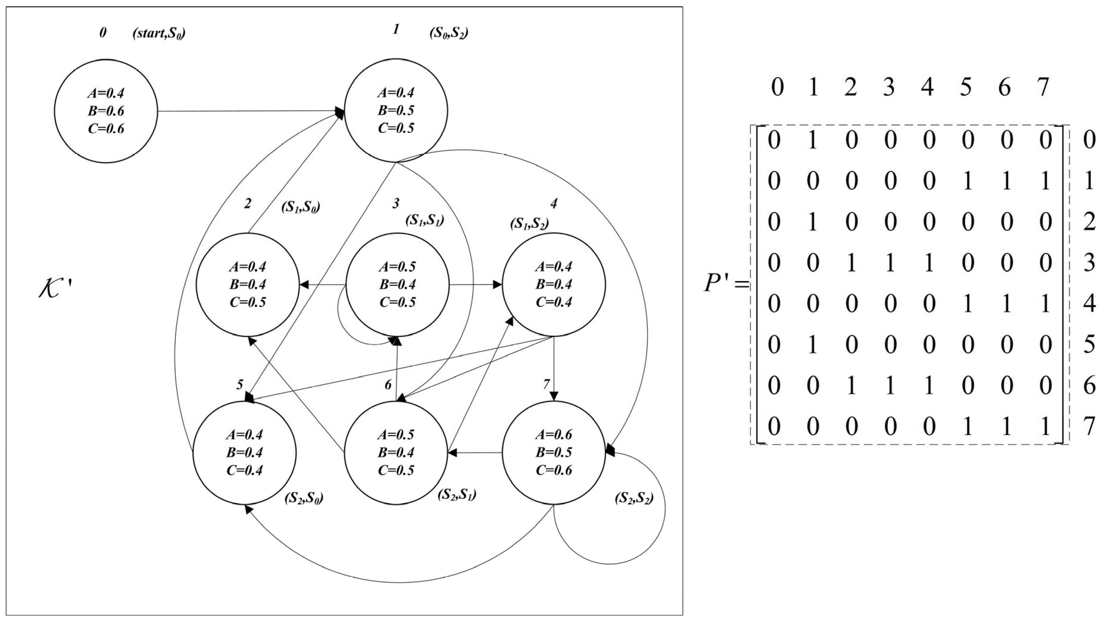
Example 2.

For the FKS $\mathcal{K}$ in Figure 1, suppose that $f=\left\{\right(A,0.5),(B,0.5),(C,0.5\left)\right\}$ and $⊳=\left\{\right(A,<),(B,\le ),(C,<\left)\right\}$.

We construct ${\mathcal{K}}^{\prime }$ where ${\mathcal{K}}^{\prime }$ and $P^{\prime }$ are shown in Figure 2, where the truth values of $x\in AP$ in states are marked in states. In addition, $s_0^{\prime }$ is the state $(start,s_0)$, i.e., state 0.

Then, we construct set $O_x$ for every $x\in AP$ and have $O_A=\{0,1,2,4,5\}$, $O_B=\{1,2,3,4,5,$$6,7\}$ and $O_C=\{4,5\}$.

Thus, we can find a path fragment in ${\mathcal{K}}^{\prime }$ passing through at least one state in each of sets $O_A$, $O_B$, and $O_C$, to find out whether there is a path fragment $\widehat{\pi }$ in $\mathcal{K}$ which makes $\mathbb{P}(\widehat{\pi },x){⊳}_{x}f\left(x\right)$ for every $x\in AP$.

3.3. Mixed Threshold Function

Here, we consider the general case which is a mixture of the upper threshold function and the lower threshold, i.e., $⊳:AP\to \{<,\le ,>,\ge \}$. Then, we can also use the Reduction 1 to find the path fragment, but we need to process ${\mathcal{K}}^{\prime }$ to meet those conditions, which require $\mathbb{P}(\widehat{\pi },x)>f\left(x\right)$ or $\mathbb{P}(\widehat{\pi },x)\ge f\left(x\right)$ for some $x\in AP$.

The process is as follows:

Reduction 2.

Let$\mathcal{K}=(S,P,s_0,L)$be an FKS with$AP=\{x_i,0\le i\}$, $f:AP\to [0,1]$be a multi-properties objective threshold function, and$⊳:AP\to \{<,\le ,>,\ge \}$be an operator function.

First, we construct $A{P}_U=\left\{x\right|{⊳}_x\in \{>,\ge \}\&x\in AP\}$ and $A{P}_B=\left\{x\right|{⊳}_x\in \{<,\le \}\&x\in AP\}$ to divide $AP$ by ⊳. Then, we construct the following FKS ${\mathcal{K}}^{″}=(S^{″},P^{″},s_0^{″},L^{″})$.

• $S^{″}\subseteq S\times S\cup \left\{(start,s_0)\right\}$,and$(s_i,s_j)\in S^{\prime }$iff$(s_i,s_j)=(start,s_0)$or:$P(s_i,s_j)>0$and$L\left(x\right)\left(s_i\right)\wedge P(s_i,s_j)\wedge L\left(x\right)\left(s_j\right){⊳}_{x}f\left(x\right)$for every$x\in A{P}_U$,
• $s_0^{″}=(start,s_0)$
• $P^{″}((s_i,s_j),(s_i^{\prime },s_j^{\prime }))=1$ iff $s_j=s_i^{\prime }$,
• $L^{″}\left(x\right)(s_i,s_j)=L\left(x\right)\left(s_i\right)\wedge P(s_i,s_j)\wedge L\left(x\right)\left(s_j\right)$ for every $x\in AP$ and $s_i,s_j\in S$,
  $L^{″}\left(x\right)(start,s_0)=1\wedge L\left(x\right)\left(s_0\right)$.

In addition, construct set$O_x$for every$x\in AP$by the following:

• $(s_i,s_j)\in O_x$ iff $L^{″}\left(x\right)(s_i,s_j){⊳}_{x}f\left(x\right)$ for every $x\in A{P}_B$.

Please note that the differences between Reduction 1 and Reduction 2 are adding restrictions in states set and the objective states sets. Then, we prove Theorem 3 to describe how to convert.

Theorem 3.

Let ${\mathcal{K}}^{″}=(S^{″},P^{″},s_0^{″},L^{″})$ and $O_x$ for every $x\in AP$ be given by Reduction 2 when applied to $\mathcal{K}=(S,P,s_0,L)$ with $AP=\{x_i,0\le i\}$, $f:AP\to [0,1]$, and $⊳:AP\to \{<,\le ,>,\ge \}$. Then, the MPOR of $\mathcal{K}$ with $AP$, f, and ⊳ returns a path if and only if $L^{″}\left(x\right)(start,s_0){⊳}_{x}f\left(x\right)$ for every $x\in A{P}_U$ and the MOSR of ${\mathcal{K}}^{″}$ with $O_x$ for every $x\in AP$ and $f:\{O_{x_1},\cdots ,O_{x_{\left|AP\right|}}\}\to 0$ returns a path.

Proof of Theorem 3. 

First, for the ‘if’ part, suppose that $L^{″}\left(x\right)(start,s_0){⊳}_{x}f\left(x\right)$ for every $x\in A{P}_U$ and the MOSR of ${\mathcal{K}}^{″}$ with $O_x$ for every $x\in AP$ and $f:\{O_{x_1},\cdots ,O_{x_{\left|AP\right|}}\}\to 0$ returns a path $(start,s_0)(s_0,s_1)(s_1,s_2)(s_2,s_3)\cdots (s_{n-1},s_n)$. Then, from the proof in Theorem 1, we can know that, in $\mathcal{K}$ for every $x\in A{P}_B$,

$$\begin{array}{c}\hfill \mathbb{P}(s_0\cdots s_n,x){⊳}_{x}f\left(x\right).\end{array}$$

In addition, from Reduction 2, we know that, for every $x\in A{P}_U$ and $0\le i\le n-1$,

$$\begin{array}{cc}\hfill L^{″}\left(x\right)(s_i,s_{i+1})& =L\left(x\right)\left(s_i\right)\wedge P(s_i,s_j)\wedge L\left(x\right)\left(s_j\right)\hfill \\ \hfill & {⊳}_{x}f\left(x\right).\hfill \end{array}$$

Thus, for every $x\in A{P}_U$,

$$\begin{array}{cc}\hfill \mathbb{P}(s_0\cdots s_n,x)& =L\left(x\right)\left(s_0\right)\underset{i=0}{\overset{n-1}{\wedge }}(P(s_i,s_{i+1})\wedge L\left(x\right)\left(s_{i+1}\right))\hfill \\ \hfill & =1\wedge L\left(x\right)\left(s_0\right)\underset{i=0}{\overset{n-1}{\wedge }}(P(s_i,s_{i+1})\wedge L\left(x\right)\left(s_{i+1}\right))\hfill \\ \hfill & =1\wedge L\left(x\right)\left(s_0\right)\wedge P(s_0,s_1)\wedge L\left(x\right)\left(s_1\right)\wedge P(s_1,s_2)\wedge L\left(x\right)\left(s_2\right)\wedge \cdots \hfill \\ \hfill & \wedge L\left(x\right)\left(s_{n-1}\right)\wedge P(s_{n-1},s_n)\wedge L\left(x\right)\left(s_n\right)\hfill \\ \hfill & =L^{″}\left(x\right)(start,s_0)\wedge L^{″}\left(x\right)(s_0,s_1)\cdots L^{″}\left(x\right)(s_{n-1},s_n)\hfill \\ \hfill & {⊳}_{x}f\left(x\right)\wedge f\left(x\right)\cdots \wedge f\left(x\right)\hfill \\ \hfill & =f\left(x\right),\hfill \end{array}$$

from the the absorption law and idempotent law of ∧ and Reduction 2.

Hence, $\mathbb{P}(s_0\cdots s_n,x){⊳}_{x}f\left(x\right)$ for every $x\in A{P}_B\cup A{P}_U=AP$, which means that the MPOR of $\mathcal{K}$ with $AP$, f, and ⊳ returns a path $s_0\cdots s_n$.

Second, for the ‘only if’ part, suppose that the MPOR of $\mathcal{K}$ with $AP$, f, and ⊳ returns a path $s_0\cdots s_n$.

Then, we can know from Definition 1 and the definition of MPOR that, for every $x\in A{P}_U$,

$$\begin{array}{cc}\hfill \mathbb{P}(s_0\cdots s_n,x)& =L\left(x\right)\left(s_0\right)\underset{i=0}{\overset{n-1}{\wedge }}(P(s_i,s_{i+1})\wedge L\left(x\right)\left(s_{i+1}\right))\hfill \\ \hfill & =1\wedge L\left(x\right)\left(s_0\right)\underset{i=0}{\overset{n-1}{\wedge }}(P(s_i,s_{i+1})\wedge L\left(x\right)\left(s_{i+1}\right))\hfill \\ \hfill & =1\wedge L\left(x\right)\left(s_0\right)\wedge L\left(x\right)\left(s_0\right)\wedge P(s_0,s_1)\wedge L\left(x\right)\left(s_1\right)\wedge \cdots \hfill \\ \hfill & \wedge L\left(x\right)\left(s_i\right)\wedge P(s_i,s_{i+1})\wedge L\left(x\right)\left(s_{i+1}\right)\wedge \cdots \hfill \\ \hfill & \wedge L\left(x\right)\left(s_{n-1}\right)\wedge P(s_{n-1},s_n)\wedge L\left(x\right)\left(s_n\right)\hfill \\ \hfill & {⊳}_{x}f\left(x\right)\hfill \end{array}$$

which means that $L^{″}\left(x\right)(start,s_0)=1\wedge L\left(x\right)\left(s_0\right){⊳}_{x}f\left(x\right)$ and $L\left(x\right)\left(s_i\right)\wedge P(s_i,s_{i+1})\wedge L\left(x\right)\left(s_{i+1}\right){⊳}_{x}f\left(x\right)$ for every $0\le i\le n-1$. Therefore, $(s_i,s_{i+1})\in S^{″}$ from Reduction 2. Hence, $(start,s_0)(s_0,s_1)(s_1,s_2)(s_2,s_3)\cdots (s_{n-1},s_n)$ is a path of ${\mathcal{K}}^{″}.$

From the proof of Theorem 1, we can obtain immediately that $(start,s_0)(s_0,s_1)\cdots (s_{n-1},s_n)$ is the returned path in the MOSR of ${\mathcal{K}}^{″}$ with $O_x$ for every $x\in AP$ and $f:\{O_{x_1},\cdots ,O_{x_{\left|AP\right|}}\}\to 0$.  □

Algorithm 2 is the pseudo code of transformation from MPOR to MOSR. Its correctness is proved by Theorem 3. Then, we analyze its complexity.

Algorithm 2 Conversion algorithm

Require:  An FKS $\mathcal{K}=(S,P,s_0,L)$ with $AP=\left\{x_i\right|0\le i\}$, a multi-properties objective threshold function $f:AP\to [0,1]$, and an operator function $⊳:AP\to \{<,\le ,>,\ge \}$ Ensure:  An FKS ${\mathcal{K}}^{″}=(S^{″},P^{″},s_0^{″},L^{″})$ with $O_x$ for every $x\in AP$  1:  Divide $AP$ into $A{P}_U$ and $A{P}_B$  2:  Compare $L\left(x\right)\left(s_i\right)\wedge P(s_i,s_j)\wedge L\left(x\right)\left(s_j\right)$ with $f\left(x\right)$ for every $x\in A{P}_U$, and construct $S^{″}$  3:  Construct $P^{″}$ based on $S^{″}$  4:  Construct $L^{″}$ for every $x\in AP$ and $s\in S^{″}$  5:  Construct $O\left[x\right]$ for every $x\in A{P}_B$

Theorem 4.

Algorithm 2 has running time $O\left(\right|P|\times |AP\left|\right)$.

Proof. 

Line 1 runs in time $O\left(\right|AP\left|\right)$. Line 2 runs in time $O\left(\right|P|\times |AP\left|\right)$. Line 3 runs in time $O\left(\right|P\left|\right)$. Line 4 runs in time $O\left(\right|P|\times |AP\left|\right)$. Line 5 runs in time $O\left(\right|P|\times |AP\left|\right)$. Thus, the running time of Algorithm is $O\left(\right|P|\times |AP\left|\right)$. □

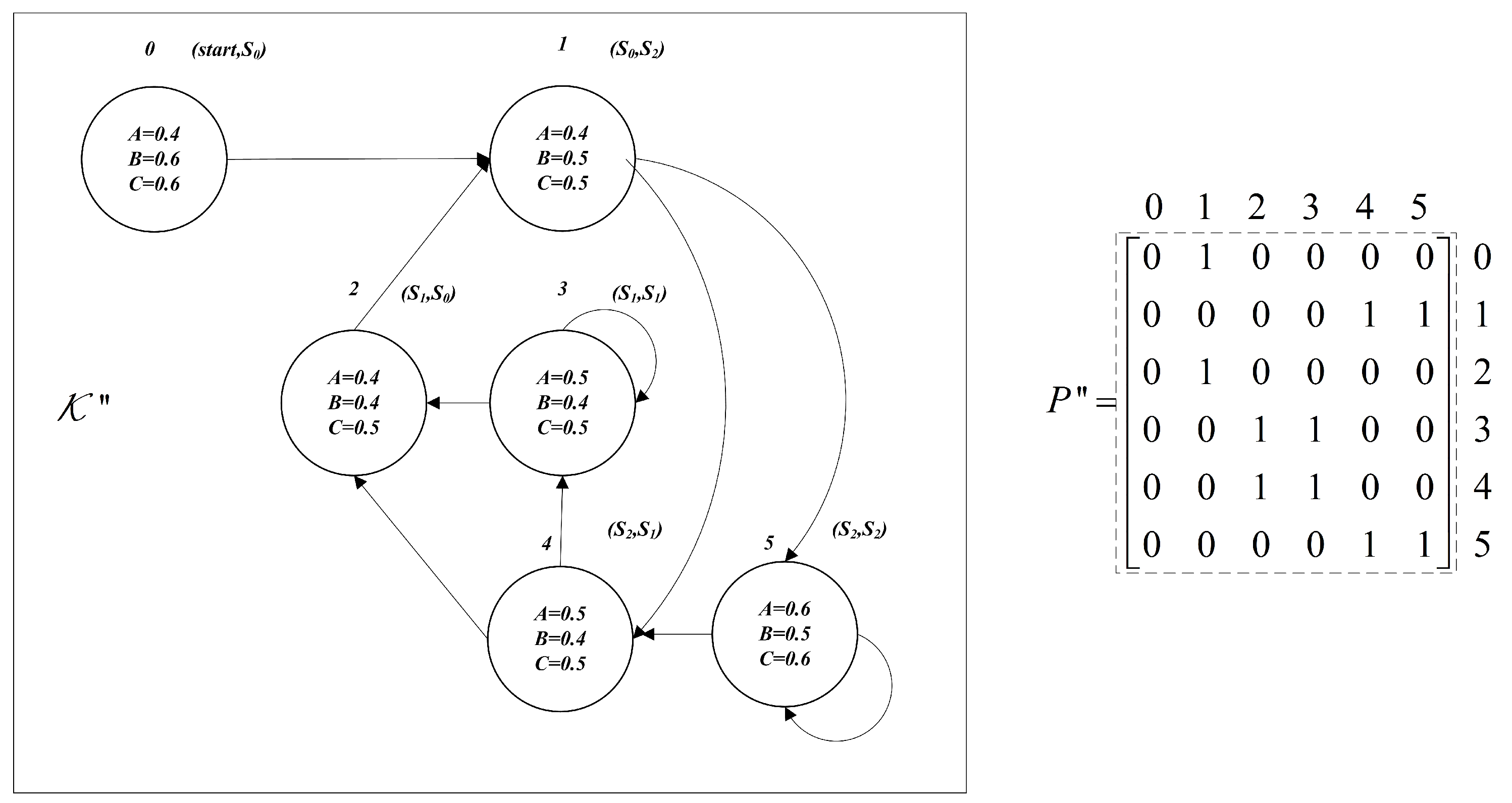
Example 3.

For the FKS $\mathcal{K}$ in Figure 1, suppose that $f=\left\{\right(A,0.5),(B,0.5),(C,0.5\left)\right\}$ and $⊳=\left\{\right(A,<),(B,\le ),(C,\ge \left)\right\}$.

First, we divide $AP$ into $A{P}_U=\left\{C\right\}$ and $A{P}_B=\{A,B\}$.

Second, we construct ${\mathcal{K}}^{″}$ where ${\mathcal{K}}^{″}$ and $P^{″}$ are shown in Figure 3, where the truth values of $x\in AP$ in states are marked in states. In addition, $s_0^{″}$ is the state $(start,s_0)$, i.e., state 0.

Then, we construct set $O_x$ for every $x\in AP$ and have $O_A=\{0,1,2\}$ and $O_B=\{1,2,3,4,5\}$.

Thus, we can find a path fragment in ${\mathcal{K}}^{\prime }$ passing through at least one state in each of sets $O_A$ and $O_B$, to find out whether there is a path fragment $\widehat{\pi }$ in $\mathcal{K}$, which makes $\mathbb{P}(\widehat{\pi },x){⊳}_{x}f\left(x\right)$ for every $x\in AP$.

4. Illustrative Example

Let us illustrate the algorithm by applying it to the disease diagnosis system studied in [24,28,32].

Assume that there is a new infectious disease in an area, where all physicians have no complete knowledge about the disease. The physicians by their experience think that some symptoms may be the features of this disease, and a treatment may be useful for treating the disease. A fuzzy Kripke structure can be used to model the treatment processes of a patient.

For simplicity, the physicians consider roughly the patient’s symptoms to be three external states: “cough”, “fever”, “diarrhea” and one internal state: “halcyon”, which are represented by C, F, D, and H, i.e., $AP=\{C,F,D,H\}$. Suppose now that there is a patient, and the physicians consider roughly the patient’s condition to be five states represented by $s_0,s_1,s_2,s_3,s_4$, i.e., $S=\{s_0,s_1,s_2,s_3,s_4\}$. According to the physicians’ estimation, the labeling function L is defined as follows:

$$\begin{array}{ccccc}\hfill & L\left(C\right)\left(s_0\right)=0.5,\hfill & \hfill L\left(F\right)\left(s_0\right)=0.7,& L\left(D\right)\left(s_0\right)=0.6,\hfill & \hfill L\left(H\right)\left(s_0\right)=0.5,\\ \hfill & L\left(C\right)\left(s_1\right)=0.4,\hfill & \hfill L\left(F\right)\left(s_1\right)=0.6,& L\left(D\right)\left(s_1\right)=0.6,\hfill & \hfill L\left(H\right)\left(s_1\right)=0.7,\\ \hfill & L\left(C\right)\left(s_2\right)=0.6,\hfill & \hfill L\left(F\right)\left(s_2\right)=0.3,& L\left(D\right)\left(s_2\right)=0.3,\hfill & \hfill L\left(H\right)\left(s_2\right)=0.3,\\ \hfill & L\left(C\right)\left(s_3\right)=0.5,\hfill & \hfill L\left(F\right)\left(s_3\right)=0.4,& L\left(D\right)\left(s_3\right)=0.5,\hfill & \hfill L\left(H\right)\left(s_3\right)=0.4,\\ \hfill & L\left(C\right)\left(s_4\right)=0.7,\hfill & \hfill L\left(F\right)\left(s_4\right)=0.5,& L\left(D\right)\left(s_4\right)=0.7,\hfill & \hfill L\left(H\right)\left(s_4\right)=0.5.\end{array}$$

Similarly, it is imprecise to say at what point exactly a patient’s condition has changed from one state to another state after the drug treatment, i.e., a treatment may lead to a state to multi-states with respective degrees. According to the physicians’ estimation, the transition possibilities after the treatment are as follows:

$$P=\left(\begin{array}{ccccc}0& 0.3& 0.6& 0.3& 0.4\\ 0.7& 0& 0.7& 0& 0.5\\ 0.4& 0.6& 0& 0& 0.6\\ 0.5& 0.6& 0& 0.7& 0.4\\ 0& 0.4& 0.3& 0.6& 0.6\end{array}\right).$$

The FKS $\mathcal{K}$ is depicted in Figure 4.

Then, we consider the following MPOR problems based on $\mathcal{K}$:

• MPOR1: $f_1=\{(C,0.3),(F,0.4),(D,0.5),(H,0.5)\}$, ${⊳}_1=\{(C,\ge ),(F,\ge ),(D,\ge ),$$(H,\ge )\}$,
• MPOR2: $f_2=\{(C,0.3),(F,0.4),(D,0.5),(H,0.5)\}$, ${⊳}_2=\{(C,\le ),(F,\le ),(D,\le ),$$(H,\le )\}$,
• MPOR3: $f_3=\{(C,0.3),(F,0.4),(D,0.5),(H,0.5)\}$, ${⊳}_3=\{(C,\ge ),(F,\ge ),(D,\le ),$$(H,\le )\}$,
• MPOR4: $f_4=\{(C,0.3),(F,0.4),(D,0.5),(H,0.5)\}$, ${⊳}_4=\{(C,\le ),(F,\le ),(D,\ge ),$$(H,\ge )\}$.

For MOSR1, because ${⊳}_1\in \{>,\ge \}$, we only compare the truth value of every $x\in AP$ in initial state $s_0$ with $f_1\left(x\right)$ and can obtain that a path fragment to this problem is $\widehat{\pi }=s_0$.

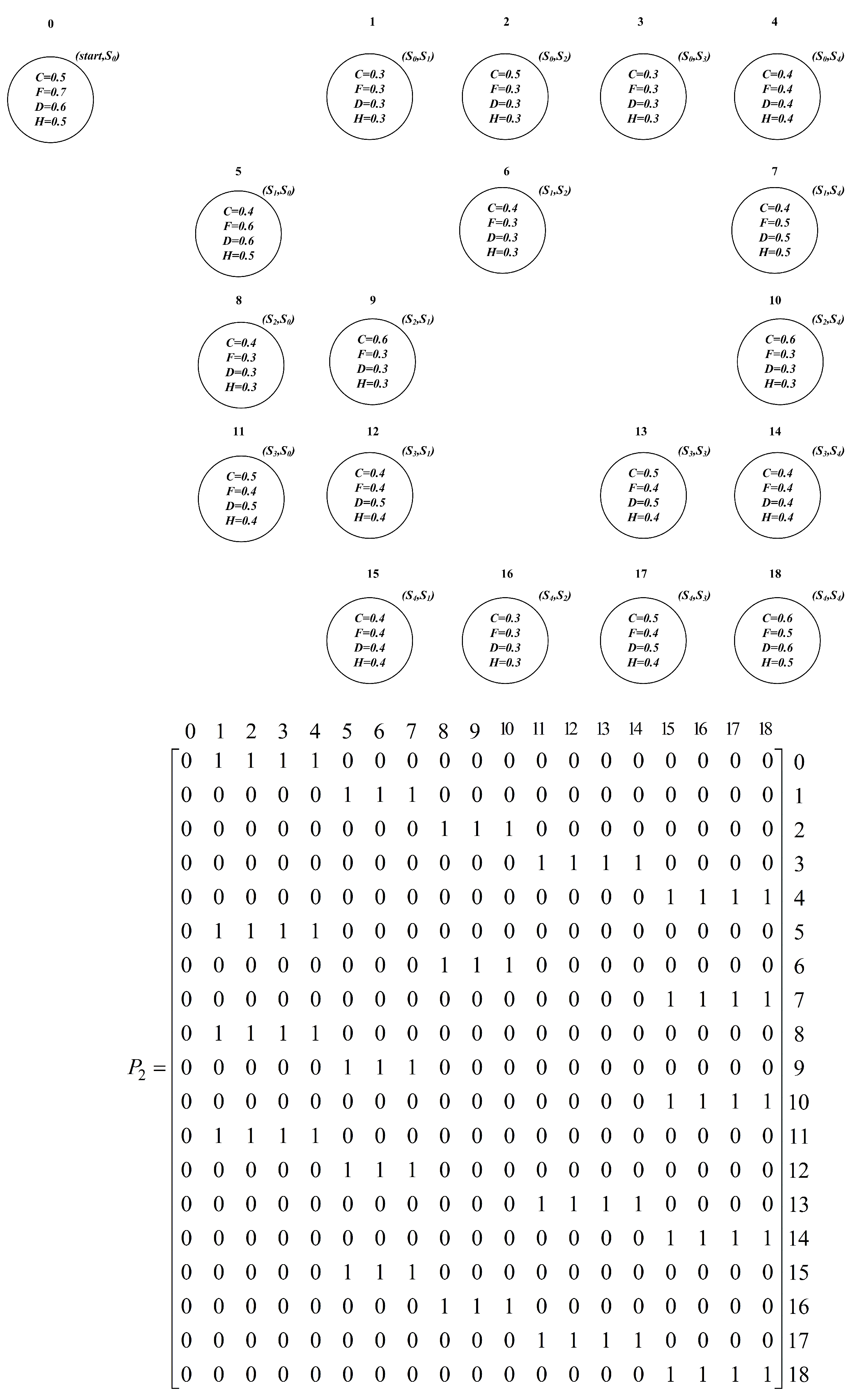
For MOSR2, because ${⊳}_2\in \{<,\le \}$, we construct ${\mathcal{K}}_2^{\prime }$ based on Reduction 1 in Figure 5, of which $S_2$ is the states set and $P_2$ is the transitions. The states set $S_2=\{0,1,2,3,4,5,6,7,8,9,$$10,11,12,13,14,15,16,17,18\}$, and the series of states sets are $O_{C2}=\{1,3,16\}$, $O_{F2}=\{1,2,3,4,6,8,9,10,11,12,13,14,15,16,17\}$, $O_{D2}=\{1,2,3,4,6,7,8,9,10,11,12,13,14,15,16,$$17\}$ and $O_{H2}=\{0,1,2,3,4,5,6,7,8,9,10,11,12,13,14,15,16,17,18\}$. We can find that $O_{H2}=S_2$, which means that $f\left(H\right)\le 0.5$ is always true during this process and can be omitted. In addition, $O_{C2}\cap O_{F2}\cap O_{D2}=\{1,3,16\}=O_{C2}$, which means that, if we passed through the process $s_0{s}_1$ or $s_0{s}_3$ or $s_4{s}_2$, the truth value will be sure to be $f\left(C\right)\le 0.3$, $f\left(F\right)\le 0.4$ and $f\left(D\right)\le 0.5$, and that, if our process makes $f\left(C\right)\le 0.3$, it will meet $f\left(F\right)\le 0.4$ and $f\left(D\right)\le 0.5$. In other words, the relationships on these sets may be used to construct and validate inference rules.

For MOSR3, because ${⊳}_3\in \{<,\le ,>,\ge \}$, we construct ${\mathcal{K}}_3^{\prime }$ based on Reduction 2 in Figure 6, of which $S_3$ is the states set and $P_3$ is the transitions. The states set $S_3=\{0,4,5,7,11,12,13,14,15,17,18\}$, and the series of states sets are $O_{D3}=\{4,7,11,12,13,14,15,$$17\}=S_3\cap O_{D2}$ and $O_{H3}=\{0,4,5,7,11,12,13,14,15,17,18\}=S_3\cap O_{H2}$, which means that perhaps we can achieve the transformation between problems through some set operations.

For MOSR4, because ${⊳}_3\in \{<,\le ,>,\ge \}$, we construct ${\mathcal{K}}_3^{\prime }$ based on Reduction 2 in Figure 7, of which $S_4$ is the states set and $P_4$ is the transitions. The states set $S_4=\{0,5,7,18\}$, and the series of states sets are $O_{C4}=\varnothing$ and $O_{F4}=\varnothing$, which means that, if we want to keep $f\left(D\right)\ge 0.5$ and $f\left(H\right)\ge 0.5$, we will always not meet $f\left(C\right)\le 0.3$ and $f\left(F\right)\le 0.4$.

5. Conclusions

In this paper, we first propose the multi-properties objective reachability problem (MPOR) and multi-objective sets reachability problem (MOSR) over FKS based on Zadeh logic. Then, we prove that a multi-properties objective reachability problem and a special case of multi-objective sets reachability problems have symmetry, and give a polynomial time algorithm based on this symmetry. Finally, we use the example of a disease diagnosis system to illustrate the process and some possible applications. The main contribution of this paper is a symmetry and a polynomial time conversion algorithm, which may be used to study the relationship between properties (MPOR) through the relationship of sets (MOSR), and establishes a link between the two multi-problems in the Zadeh fuzzy scene.

At the beginning, we were prepared to prove that these two multi-problems were equivalent in the Zadeh fuzzy scene. However, we find that the multi-objective sets reachability problem is more complex. Next, we will focus on the multi-objective sets reachability problem. In addition, there are several problems that are worthy of further study. One of the directions is to systematically investigate the method of studying property relationships through sets. Another direction is to extend Zadeh fuzzy logic to t-norm fuzzy logic. In addition, the study of whether there is a method through which we can transmit the set problems to property problems under some special cases is possible. In addition, it can be studied how to use MPOR, MOSR, and their relationships to solve fuzzy equations and fuzzy inequalities.