Abstract
As we know, image colorization is widely used in computer graphics and has become a research hotspot in the field of image processing. Current image colorization technology has the phenomenon of single coloring effect and unreal color, which is too complicated to be implemented and struggled to gain popularity. In this paper, a new method based on a convolution neural network is proposed to study the reasonable coloring of human images and ensures the realism of the coloring effect and the diversity of coloring at the same time. First, this paper selects about 5000 pictures of people and plants from the Imagenet dataset and makes a small dataset containing only people and backgrounds. Secondly, in order to obtain the image segmentation results, this paper improves the U-net network and carries out three times of down sampling and three times of up-sampling. Finally, we add the expanded convolution, and use the sigmoid activation function to replace the ReLU (The Rectified Linear Unit) activation function and put the BN (Batch Normalization) before the activation function. Experimental results show that our proposed image colorization algorithm based on the deep learning scheme can reduce the training time of the network and achieve higher quality segmentation results.
1. Introduction
Although black-and-white photos are precious to the preservation, they are very dim and lifeless. Compared with black-and-white pictures, colorization, which gives people an immersive feeling, can make the picture look more vivid and real, and shows the significance of its shooting more vividly. It is not difficult to convert a color image directly to black-and-white, but the reverse process is more difficult. Without any reference, the color is dependent upon imagination, and sometimes the coloring results are very unrealistic. Coloring technology is under a very long history. In the early days, people painted their favorite colors on black-and-white images by hand. Later, black-and-white films evolved into color images, and the image coloring technology became more and more mature. In general, colorization methods can be broadly classified into the following two main classes: interactive colorization methods and automatic colorization methods [1]. Interactive colorization technique [2,3,4,5] requires users to control the display of objects in interactive mode, such as the transformation, camera navigation, and playback. Unfortunately, this method depends on the user’s familiarity with the level of the mark color on the target image or the image segmentation. Generally, it is difficult for novices to complete the color marking or image segmentation on the target image, so it is very difficult to realize the interactive coloring method. Automatic colorization methods include a variety of image colorization methods, such as pixel-wise classification and regression [6], joint end-to-end learning of global and local image priors method [7], Convolutional Neural Network [8,9] and so on. These methods require users to convert the input reference color images into the target images, which can greatly reduce the error caused by human factors. Usually, users need to adjust the parameters to obtain the desired results.
With the development of deep learning in recent years, various kinds of deep neural network models are emerging. These models can extract complex features for different application scenarios and complete some intelligent corresponding tasks. Thakur et al. [10] applied deep learning to smart homes under the Internet of Things, and used big data and machine learning methods to locate users indoors. Rahim et al. [11] analyzed the recent development of COVID-19 in Australia, Italy and the United Kingdom and applied the deep learning algorithm to establish a variety of case models to predict epidemiology in the above-mentioned countries. Through the accumulation and analysis of a large number of image data information features, deep learning can automatically complete the tasks of feature extraction and image matching. In recent decades, image coloring has always been the research hotspot of computer graphics. In the field of deep learning, many neural networks for coloring research have emerged, including deep learning networks, recursive neural networks, and deep belief networks. Cheng et al. [12] proposed a coloring algorithm based on a convolutional neural network. They trained a neural network using a large set of example reference images and used the learned neural network to colorize a target grayscale image. Because the algorithm uses DAISY [13] which relies on machine learning techniques and other features to describe, it cannot achieve complete end-to-end automatic image coloring, and the entire coloring process is relatively inefficient. Cao et al. [14] used conditional generative adversarial networks for the colorization of grayscale images. They developed a fully convolutional generator and introduced the input noise and the gray level image into the first several layers of the network of the generator, and the multi-layer noise was sampled to achieve a variety of shading effects. Unfortunately, the disadvantage of generating the confrontation framework is that the model involves the training of two networks, and it is prone to the problem of poor stability. Liu et al. [15] proposed an auto-painter model to solve the coloring problem of black-and-white cartoons by using conditional generative adversarial networks. However, they encounter difficulties in adjusting parameters, and the complex network structure may lead to low training efficiency. Guadarrama et al. [16] used the PixelCNN model to solve the gray image coloring problem. They generated a chroma prediction image with lower resolution than the gray image through experiments, and then passed the color image with lower resolution and the original gray image through a correction network. The original gray level image combines the chrominance information with low resolution to generate a color image with the same resolution as the input gray image. Su et al. [17] proposed a method for achieving instance-aware colorization. The network consists of an off-the-shelf pre-trained model, two colored networks for training background and instances, respectively, and a module for fusing extracted features. In this method, the instance object and background are trained separately, and then the instance feature and background feature are mixed through the fusion module to obtain the final color output. This method effectively improves the effect of shading. However, the color difference between foreground instances and background in some images is evident, and there is a problem of inconsistent main colors. Patricia et al. [18] proposed an adversarial learning colorization approach coupled with semantic information. This method integrates the scene classification into the generation countermeasure network, and realizes the grayscale image coloring by sensing the scene category and color information. The color of the color image generated by this method has a certain sense of reality, but there is always a problem of insufficient detail information. Gao et al. [19] proposed an end-to-end image colorization framework. They believed that the color prominent areas of the image determine the quality of the color image and add the Adaptive Group Instance Normalization (AGIN) function to the algorithm to promote color rendering. Of course, convolutional neural networks are used most, because when the input and output of the network are images, the network is demonstrated to have the best effect [20,21]. The colorization algorithm based on convolutional neural network has achieved excellent results. However, it is trained in a large data set and the images are complex and diverse without specificity; the coloring effect for the human image is not ideal. We have made some improvements on character coloring. When the training target changes, the depth, loss function and activation function of the network can be modified to obtain better results. Aiming at the problem that the current image coloring effect is not ideal, and the color is single, combined with the requirements that people need to achieve real-time interaction, diversity, and authenticity for the coloring of black-and-white people’s photos. This paper improves the U-net network to accurately extract the features of the people’s images from the production of new data sets. By predicting the probability distribution of possible colors and human interaction, a variety of reasonable coloring effects can be obtained in real time.
2. Related Works
2.1. Colorization Method Based on Local Color
Because the human eye is controlled by the nervous system, the number of distinguishable levels of the human eye for the gray-scale scene under the same brightness background is far lower than the number of color distinguishable levels for different brightness and chroma. In order to help the public better understand the photo or video scene, more and more scholars pay attention to the colorization of gray-scale images. Early image colorization methods focused on pixel points of marker color provided by users, and transmitted color information manually marked on the whole image through the colorization of the gray-scale image; spots of different colors were applied to an image with various colors. Image colorization technology is a challenging research topic in the field of digital image processing and computer vision. It can not only provide effective solutions for image enhancement and image segmentation, but also has very broad application prospects in the fields of black-and-white film and television data restoration, animation production, infrared image visualization, biomedical imaging, and so on.
Levin et al. [22] first assumed that neighboring pixels in space-time that have similar intensities should have similar colors. They formalized the premise using a quadratic cost function and obtained an optimization problem that could be solved efficiently using standard techniques. The method proposed by Yatziv et al. [23] was fast and permitted the user to interactively get the desired results promptly after providing a reduced set of chrominance scribbles. Sangkloy et al. [24] proposed a deep adversarial image synthesis architecture, which demonstrated a sketch-based image synthesis system which allows users to ‘scribble’ over the sketch to indicate the preferred color for objects. The coloring method based on local color is suitable for simple image coloring tasks, but when users perform coloring tasks for complex images and large-scale images, the coloring efficiency is low. Unfortunately, this algorithm requires a lot of manual editing to perform color propagation according to the color information of the annotation, so as to complete the coloring task of the global image. This method requires the user to have enough art skills to ensure that the coloring results are accurate and reasonable. Because the coloring effect of an image is completely determined by the color information marked by the user, if the marked area or color is not accurate, image distortion is likely to occur.
2.2. Color Transfer Method
Reinhard et al. [25] used a simple statistical analysis to impose one image’s color characteristics on another. They used statistical algorithms to find similar pixels in the reference image set that are consistent with the target image, and assigned the color characteristics of the reference image to the target image. Welsh et al. [26] introduced a general technique for colorizing greyscale images by transferring color between a source, color image and a destination, greyscale image. However, the premise of this method is the case that the texture and brightness should be sufficiently distinct. The disadvantage of this method is that it makes it easy for the color to cross the boundary. Compared to the vegetation with clear texture and obvious color, the shading effect is relatively good, but it is not ideal for the image with less clear texture. Xiang et al. [27] presented an improved EM method to model regional color distribution of the target image by the Gaussian Mixture Model (GMM), then, trained by this model, appropriate reference colors were automatically selected from the given source images to color each target region. However, the effect of the transfer is somewhat ambiguous. Only when the input and reference shared content are similar, the effect of this method may appear unnatural. Irony et al. [28] presented a new method for colorizing grayscale images by transferring color from a segmented example image. Chia et al. [29] proposed a colorization system that leverages the rich image content on the internet. Cascade feature matching was utilized to find the mapping relationship between the reference image and the super pixels of the target image. The coloring effect of the color transfer method was based on the richness of the color of the selected sample image and the feature matching method of pixel points between the reference image and the target image during the color transfer. Only a few steps of this kind of method require the involvement of users, and the professional level of users is relatively low. The qualitative comparison of color transfer results is indicated in Figure 1.

Figure 1.
Qualitative comparison of color transfer results: (a) Gray scale picture; (b) Reference diagram; (c) Transfer effect; (d) Proposed. It can be observed that the effect of the color transfer method is not ideal, and there is a phenomenon that the color goes beyond the boundary to the background. The algorithm in this paper has a great effect.
2.3. Fully Automatic Colorization
With the rapid development of deep learning techniques, more and more scholars give attention to machine learning and deep learning technology. A fully automatic colorization method is proposed without any reference image. Rizzi et al. [30] presented an algorithm called Automatic Color Equalization for digital images which has unsupervised enhancement with simultaneous global and local effects. Morimoto et al. [31] proposed an automatic coloring method for multiple images gathered from the Web. This method uses the information of the scene structure to retrieve the images to be colored in the image library and transfer colors, so as to generate various color images. Cohen-Or et al. [32] presented a method that enhances the harmony among the colors of a given photograph or of a general image, while remaining faithful to the original colors as much as possible. Bychkovsky et al. [33] created a high-quality reference dataset to learn an automatic model of tone adjustment in the luminance channel. Yan et al. [34] explored the use of deep neural networks (DNNs) in the context of photo editing. The photos are artistically enhanced through style color and tone adjustment to bring out vivid visual impression, but the automatic color adjustment is mainly carried out for color pictures. However, when this algorithm is used in the real-time neural network of the output layer of the spatiotemporal context, the pre-trained data may be replaced by a large number of training data, which may lead to the distortion of the image color. Larsson et al. [35] trained a model to predict per-pixel color histograms as many scene elements naturally appear according to multimodal color distributions. Qin et al. [36] proposed an image colorization method based on a deep residual neural network. This method combines the classified information and features of the image, uses the whole image as the input of the network, and forms a non-linear mapping from grayscale images to the colorful images through the deep network. Figure 2 illustrates affecting coloration of fully automatic colorization.

Figure 2.
Affecting coloration of fully automatic colorization. (a) Reality image; (b) Bychkovsky et al. [33]; (c) Yan et al. [34]. From (b) and (c), it can be seen that the color of the image is somewhat exaggerated and does not match the actual color effect.
3. Proposed Method
In this paper, we present an improved U-net network called CU-net to improve the quality of the coloring algorithm. CU-net is used to enhance the deep restoration of image realism in view of the common problems of current colorization methods in Section 2.1, Section 2.2 and Section 2.3. By improving the structure of u network, the problem of gradient disappearance or explosion is effectively solved, and the feature utilization rate is further improved. The proposed scheme mainly consists of four phases: (1) the data set is introduced, (2) an improved U-net network is proposed, (3) the learning process of the main coloring network is described, and (4) the color space conversion of color map generation is introduced.
3.1. Dataset
Imagenet project is a large-scale visualization database for image recognition software research, and it is also a huge picture library for image training. It is the primary choice for numerous convolutional neural network datasets [37], because it is the largest database for image recognition in the world. The Imagenet dataset covers 22,000 items and contains 15 million photos. However, this paper mainly studies the coloring problem of people pictures, the dataset only involves people and some backgrounds without a large amount of data. Download the Imagenet data set on the official website, which contains many files. Although there are almost one million picture data on the disk, there is no intuitive name and no obvious way to know the label information corresponding to each image. Next, we need to find the corresponding picture category.
First, extract the file: tar-xvf ilsvrc2016_ CLS-LOC. tar. GZ, after decompression, a directory named ilsvrc is obtained, which has three subdirectories named annotations, data, and imagesets. Annotations is the object location annotation data file, which is commonly used in object detection tasks. At present, this folder can be ignored. The data folder, which is the focus of this article to obtain the data set, contains the original image data of train, Val and test. Imagesets refer to attributes of information corresponding to the image. This article mainly uses the data directory. Table 1 shows three subdirectories of Ilsvrc.

Table 1.
Three subdirectories of Ilsvrc.
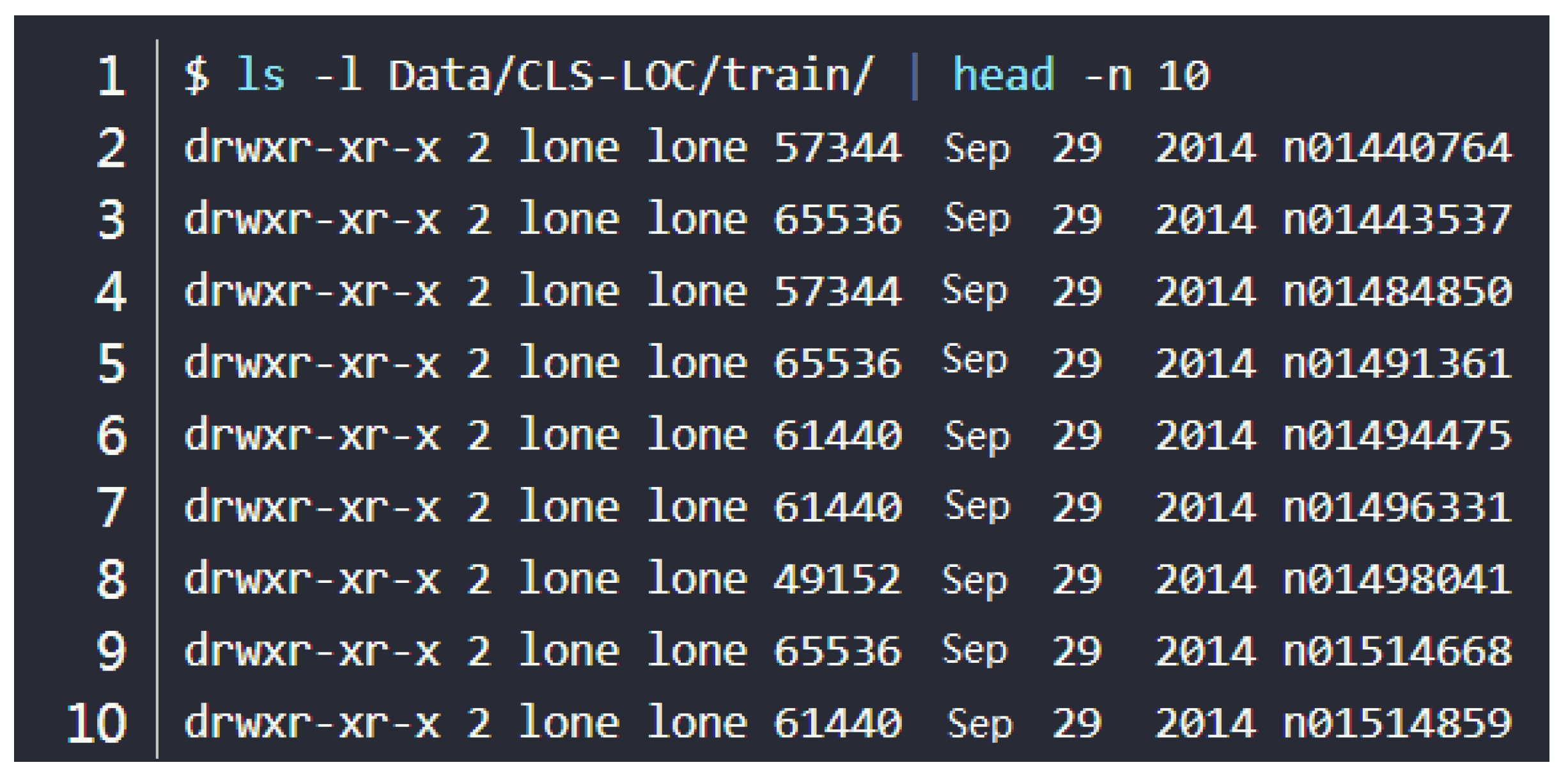
The train directory consists of a series of subdirectories, as shown in Figure 3.
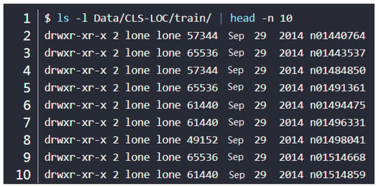
Figure 3.
Train directory in Imagenet. This paper mainly uses the data directory. The train directory is a series of subdirectories.
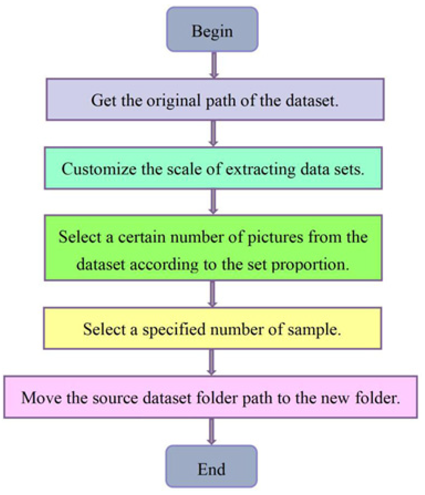
These directory names do not appear to contain any image information. In fact, Imagenet datasets are mapped according to WordNet IDS, which are called synonym sets or simply “synsets”. Each ID maps to a specific data tag, such as a person, a sport, an airplane, or a guitar. Therefore, these file names are actually WordNet IDS corresponding to each class, and in these tag subdirectories, there are about 732 to 1300 images per class. For example, the subdirectory with WordNet ID n01440764 contains 1300 images of “Tenth”, a European freshwater fish. The part selected in this paper is the WordNet ID n00007846 containing people, from which more than 4000 photos are randomly selected. The process of obtaining a sample picture of a person is as follows. First, we get the original path of the dataset. WordNet ID of the dataset mentioned here is n00007846. Secondly, the scale of extracting datasets is customized. For example, 20 out of 100 is 20%. Thirdly, we select a certain number of pictures from the dataset according to the set proportion. Fourthly, a specified number of the sample is selected from the picture obtained in the previous step. Lastly, we move the source dataset folder path to the new folder and get the required character samples. Figure 4 shows the process of randomly selecting batch images.
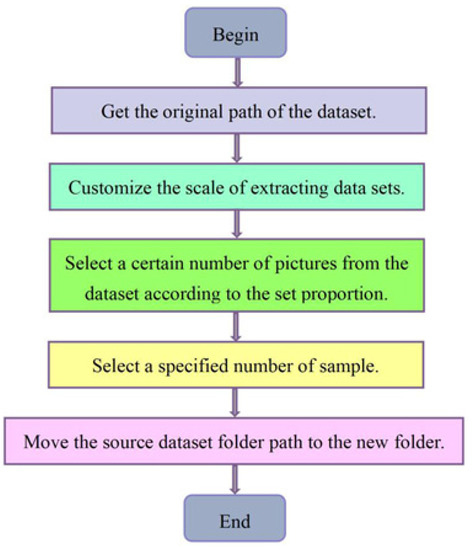
Figure 4.
The process of randomly selecting batch images.
3.2. Improved U-Net Network
U-Net is a CNN architecture formed by a symmetrical encoder–decoder backbone with skip connection that is widely used for automated image segmentation and has demonstrated remarkable performance [38,39]. U-Net is a symmetrical network structure. Its core idea is to first realize down-sampling to reduce the size of the image, extract feature information through the convolution basis superimposed by the convolution layer and the pool layer, and then use the transposed convolution to recover the feature size in the up-sampling stage. The number of channels of the image is halved. In the down sampling stage, the context features are captured to accurately locate. Jump connection fuses the feature map of each layer sampled down with the feature map of the corresponding layer sampled up. Input the fused feature map into two convolution layers and the activation function until the output feature map has the same size ratio with the input, and the segmented image can be achieved. The feature fusion mode of U-Net network differs from that of Full Convolutional Networks for Semantic Segmentation (FCN). The difference is that FCN simply adds features of different scales, while U-Net network combines the low-resolution information of down sampling and the high-resolution information of up-sampling. Its jump connection is to splice the feature information according to the channel dimension. It effectively connects the feature information of coding path and decoding path, fills in the underlying information, and improves the training accuracy. Compared with FCN, U-Net can obtain more refined training effects. Because U-Net also shows excellent performance on small data sets, it is commonly used in image processing. Because U-Net needs to classify each pixel in each image, it will cause a lot of redundancy due to a large number of repeated feature extraction processes while forming a huge amount of computation, which will eventually lead to low training efficiency of the entire network. Furthermore, when data samples are heavy, using a large number of pooling operations will reduce the dimension of each feature map, resulting in the loss of much valuable information. In the process of encoding and decoding of U-net network, successive up- and down-sampling operations will lead to the loss of valuable detailed information, which leads to imperfect segmentation accuracy. Moreover, U-net is not clear in identifying background targets, such as being inadequate in identifying minor targets and fuzzy targets.
In order to obtain a feature layer with richer global semantic information and a greater receptive field, we reduce the model parameters by reducing the depth of the network, introduce expansion convolution and remove the maximum pooling link, and add symmetrical jump connections to the corresponding convolution and transposition convolution layers, so that the network can better obtain more important feature information of the feature layer, and reduce training time without losing the model segmentation accuracy. The above methods enable the new model to achieve better coloring results on black and white person photos, which is called CU-net. This paper proposes an improved convolutional neural network model CU-net, based on U-net as the main network framework of this paper. U-net has the ability of local perception, which is suitable for small data sets, and the network structure is simple. It can obtain a better segmentation effect in the case of a short training time. We have made the following improvements to U-net: we complete three down-sampling and three up-sampling in order to decrease the depth of the network. It is worth mentioning that in the down-sampling process, the maximum pooling operation is removed and the dilated convolution is introduced.
As shown in Figure 5, the CU-net network is mainly divided into two parts, which are the down-sampling and the up-sampling. The down-sampling is a process from high resolution (shallow features) to low resolution (deep features), while the up-sampling restores the feature resolution of the image. For the feature extraction stage, the shallow structure can capture some simple features of the human image, such as the contour of the human body and the local boundary, while the deep structure can capture some subtle features of the image, such as the head and neck, because the perception field is large and the convolution operation is more. Through the improvement, a network structure integrating detection, classification and segmentation will be obtained. The network is composed of 10 convolution blocks conv1-10. It mainly consists of down sampling, expansion convolution, up-sampling, and fast connection.
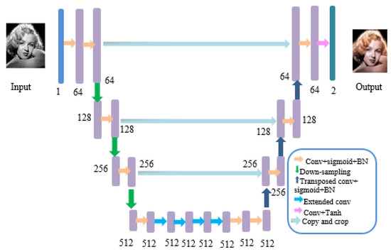
Figure 5.
The Network diagram of CU-net.
3.2.1. Down-Sampling Process
The feature extraction part is mainly implemented in the down sampling stage and distributed in each block of conv1-4. In the conv1-4 block, the convolution kernel is 3 × 3. The convolution step size is 1. The filling is 1, and then the sigmoid (SIG) activation function is used after each convolution, and a batch normalization layer (BN) is followed before each activation. Each convolution block contains two conv BN sig pairs, which realizes the gradual reduction of the feature channel in space and doubling in the feature dimension.
The purpose of Down-sampling is to make the person image conform to the size of the display area and generate a thumbnail of the corresponding image. For an image X, which size is H × W, its resolution image which size is (H/s) × (W/s) can be obtained after the s-fold down-sampling processes. When the image is in matrix form, the original image s × s window is changed into a pixel, and the value of this pixel point is the average value of all pixels in the window:
Figure 6 shows the convolution process.

Figure 6.
The convolution process. A 3 × 3 convolution kernel in 5 × 5 image is performed a convolution process with a step size of 1. Each convolution is a feature extraction method, which filters out the qualified parts in the image.
3.2.2. Introducing Extended Convolution
In order to better acquire the image features and recover the feature details of the pictures lost by down-sampling, we expanded the receptive field of the original network without losing the spatial resolution of the image, and used expanded convolution [40] in conv5-6 to remove the maximum pooling link. As we all know, the perceptual domain affects the degree of using context information, and context information is of great importance for accurate segmentation. Compared with ordinary convolution, expansion convolution has a dilation rate parameter in addition to the size of the convolution kernel, which is mainly used to represent the size of expansion. Two expanded convolutions are expanded where the kernel sizes are all 3 × 3. The dilated rate is 2. The convolution step size is 1, and the filling is 2. Then, the sigmoid (SIG) activation function is used after each convolution, and a batch normalization layer (BN) is followed before each activation. Each convolution block contains 2 conv BN sig pairs. The receptive field is the area size mapped on the original image by pixel points on the feature map output by each layer of the convolutional neural network. The calculation formula of receptive field of the convolutional a neural network is:
The receptive field of this layer is labeled r. M is the receptive field of the upper layer, stride is the step size of convolution, and k_ size is the convolution kernel size. The initial receptive field size is 1. The size of traditional receptive field is the convolution kernel, and the size is 3 × 3. Stripe = 1. The receptive field obtained by changing the step size is given in Table 2.

Table 2.
Traditional receptive field calculation process.
Comparing the change of the receptive field of cavity convolution, the convolution kernel size is 3 × 3, stripe = 1 and 2, padding = 1, as showed in Table 3 and Table 4.

Table 3.
The size of the receptive field of the expansion rate changes (stride = 1).

Table 4.
The size of the receptive field of the expansion rate changes (stride = 2).
3.2.3. Up-Sampling Process
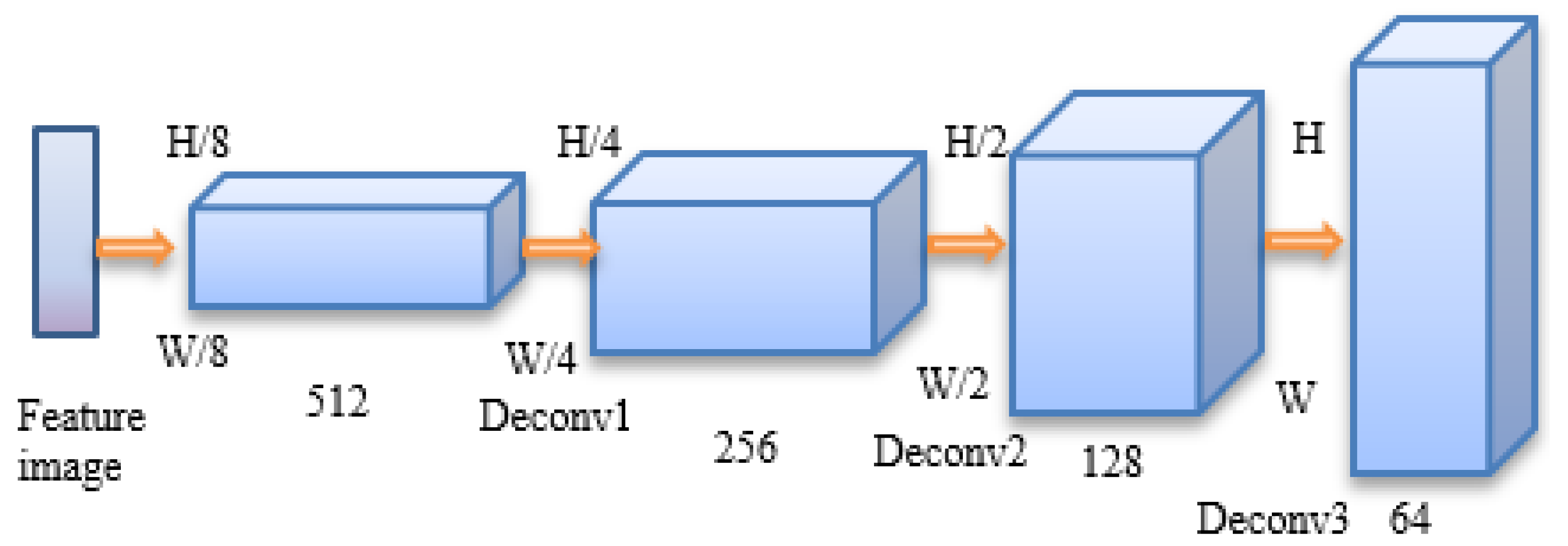
In order to enlarge the feature map of the image, the redundant part is cut off with the clipping layer to make it have the same size as the actual image so as to calculate the predicted value of each pixel. In the conv7 block, the convolution kernel is 3 × 3. The convolution step size is 1 and the filling is 1. Then, sigmoid (SIG) activation function is used after each convolution, and a batch normalization layer (BN) is followed before each activation. Each convolution block contains 3 conv BN sig pairs. In the conv8-10 block, transposed convolution is utilized to perform the reverse operation on the convolution in the neural network structure. In the first several convolution layers, the transposed convolution kernel is 4 × 4. The convolution step size is 2 and the filling is 1, followed by the same convolution kernel, step size, and filling as the first convolution block. Then, sigmoid activation function and batch normalized BN processing is used. Each convolution block contains two conv–BN sig pairs. After three times of transposition convolution operation with a step size of 2, the spatial resolution of the feature map is slowly restored, and the number of channels will be doubled every time the transposition convolution is performed. Finally, H × W size image is obtained. The up-sampling process using transposition convolution is given in Figure 7.
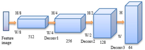
Figure 7.
Schematic diagram of the up-sampling process.
In order to communicate multiple channels and enable them to perform a linear combination in the channel dimension, the convolution operation is finally 1 × 1 convolution kernel instead of performing a single channel convolution operation. This is the information exchange between channels.
3.2.4. Symmetric Skip Connection
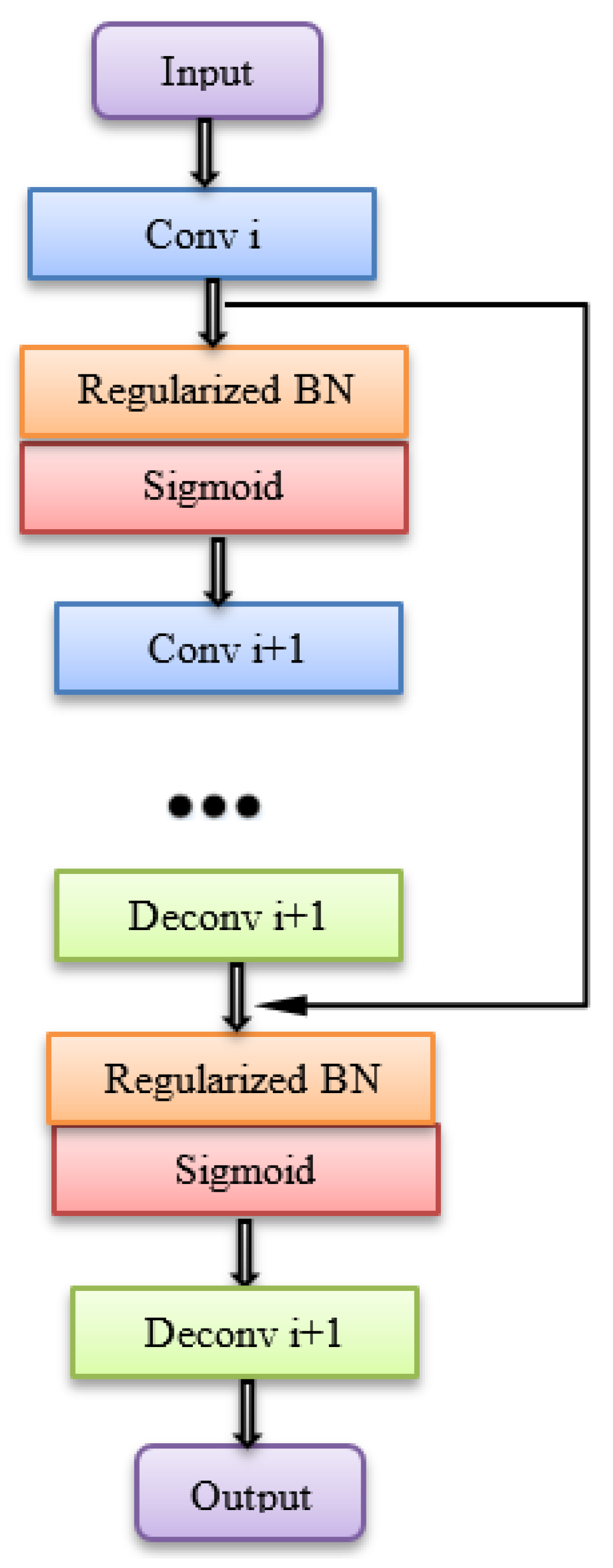
When the deep neural network is trained, the performance of the model may decrease with the increase of the architecture depth. As the depth of the architecture increases, the model tends to over fit. On the other hand, when sigmoid is invoked as the loss function, the gradient cannot exceed 0.25. After chain derivation, the hidden layer weights close to the input layer will be updated slowly or stagnated, and the gradient will easily disappear. The gradient explosion generally occurs when the initialization value of the deep network and the weight is too large. If the gradient value between the network layers is greater than 1.0, the repeated multiplication will cause the gradient to increase exponentially, and the gradient will become very heavy. Then, network weight will be greatly updated, and the network will become unstable. For a more accurate feature extraction, symmetric skip connection is added, and concat is used to connect the corresponding convolution and transposition convolution layers to help the network recover spatial information. The network contains symmetric convolution and deconvolution layers, and every few layers have jump connections from the convolution feature map to the corresponding deconvolution feature map. In this paper, conv2 and conv3 blocks are connected to conv8 and conv9 blocks respectively. The detailed low-level image information is transferred to the subsequent layer, which also makes the important low-level information of the subsequent layer easy to access and provides a path for the flow of data signals, so as to effectively solve the gradient disappearance or explosion problem. The experimental results show that this method is superior to the prior art in image denoising and super-resolution. In order to better train the deep network, we add skip connections between the corresponding convolution layer and the deconvolution layer. These skip connections serve to transfer the gradient to the bottom layer and make the data signal flow smoothly in the path. The flow chart of symmetric skip connection process is illustrated in Figure 8.

Figure 8.
Flow chart of symmetric skip connection process.
Finally, the detailed network structure of each part is given, as shown in Table 5, Table 6, Table 7 and Table 8. Conv bottle indicates the serial number, conv1-1 in type indicates the number of channels corresponding to the input and output images of the convolution kernel, and the same applies to others. Kernel indicates 3 × 3 convolution kernels. Stripe represents the sampling interval during convolution. Padding represents the number of rows or columns added to the edge of the input feature map, and channel represents the number of feature maps after each convolution. Table 5 shows the down-sampling network structure. Table 6 displays the extended network structure. Table 7 displays the up-sampling network structure. Table 8 displays the symmetrical connection structure.

Table 5.
Down-sampling network structure.

Table 6.
Expand network structure.

Table 7.
Up-sampling network structure.

Table 8.
Symmetrical connection structure.
3.2.5. Activation Function and Batch Normalization
It is particularly important for image segmentation to fuse low-level features and high-level features and effectively propagate them back to all layers, which are related to the final coloring of the image. Because of the channel number of feature pixels, the resolution is distinct in different feature fusion layers, and the shallower the layer, the larger the scale. Before fusing low-level features and high-level features of different sizes, the output features of each layer need to be batch-standardized. First of all, normalization is to subtract the mean value from the input value of the data and then divide it by the standard deviation of the data. Image processing is a process of feature extraction layer by layer, and the output of each layer can be interpreted as the data after feature extraction. Therefore, normalization means that data normalization is performed at each layer of the network. However, such an operation is computationally expensive, just like using minimum batch gradient descent. The “batch” in batch normalization actually refers to sampling a small batch of data, and then normalizing the output of the batch of data at each layer of the network [41]. In this way, the problems of uneven distribution and “gradient dispersion” of each layer can be solved, and the network training can be accelerated.
Assume several pieces of data are employed to one sampling training. is the mean of the output value of the neuron model of layer j when the kth data is trained. represents the average output value of this batch of data at the I neurons of layer J. represents the standard deviation of the output value of this batch of data at the i-neuron type of layer J. The output value after batch normalization is as follows:
The mean value of neuron type output is measured by:
The standard deviation of neuron output value is measured by:
where is a very small constant to prevent the denominator of Formula (3) from tending to 0. The purpose of batch normalization is actually very simple, that is, to adjust the input data of each layer of the neural network to the standard normal distribution with the mean value of zero and the variance of 1. In order to solve the gradient saturation problem, ReLU activation function is used. Generally, batch normalization (BN) operation is added to large training data sets and deep neural networks. Compared with the shallow neural networks including three down-sampling and three up-sampling processes, and small data sets, sigmoid activation is more suitable for this paper. Sigmoid function has an exponential form as follows:
The main reason for using a sigmoid function is that it exists between 0 and 1, which is convenient for the derivation. Therefore, it is applicable to the model that must predict the probability as the output. Since the probability of anything only exists between 0 and 1, sigmoid is the correct choice. When the output value is large, the sigmoid function will enter the saturation region, resulting in its derivative being almost zero. Even if we know that the neuron needs to be corrected, the gradient will be too small to train. The value of sigmoid activation function between [–2, 2] is an approximately linear region. Therefore, what this paper does is to put the batch standardized transformation before the activation function, which is equivalent to adding a preprocessing operation at the input of each layer, and then entering the next layer of the network, as showed in Figure 9.

Figure 9.
Batch standardization location.
What the BN algorithm does is to normalize the input value as much as possible in the narrow area of sigmoid activation function [–2, 2]. As |x| increases, s’(x) tends to zero.
Since x is affected by W, b and the parameters of all the layers below, changes to those parameters during training will likely move many dimensions of x into the saturated regime of the nonlinearity and slow down the convergence. The change in the distribution of internal nodes in the deep network during the training process is called the internal covariate shift, which is defined as the change in the network activation distribution caused by the change of network parameters during the training. In order to improve training, we sought to reduce changes in internal covariates. The training speed is expected to be improved by fixing the distribution of layer inputs during the training.
To prevent each dimension from being malicious, we normalize each scalar feature independently, by making it have the mean of zero and the variance of 1. For a layer with d-dimensional input, each dimension is expressed as:
where the expectation and variance are computed over the training data set. For an input x with dimension d, it is necessary to standardize each dimension. Suppose that the x we input is an RGB three channel color images, then d here is the channels of the input image, that means d = 3. Standardized processing refers to processing R channel, G channel and B channel respectively. is the average value of each batch of training data neurons , while is the standard deviation of activation of each batch of neurons. The distribution of any value of has an expected value of 0 and a variance of 1, which can be obtained by observation:
The proof process of Formula (8) is given below. Let the mean value of the sample be , and its expression is
Let be the original standard deviation and be the variance, and we can acquire the equation
Let represent the changed :
Therefore
If we bring Equation (12) into Equation (13), we get
Simply normalizing the input of each layer may change what the layer can represent. For example, normalized sigmoid input constrains them to nonlinear linear states. In order to solve this problem, the parameter and the parameter are introduced for each A. They are learnable parameters, similar to weights and offsets, and are generally updated by gradient descent method. They scale and shift the normalized values:
these parameters are learned together with the original model parameters and the representation ability of the network is restored.
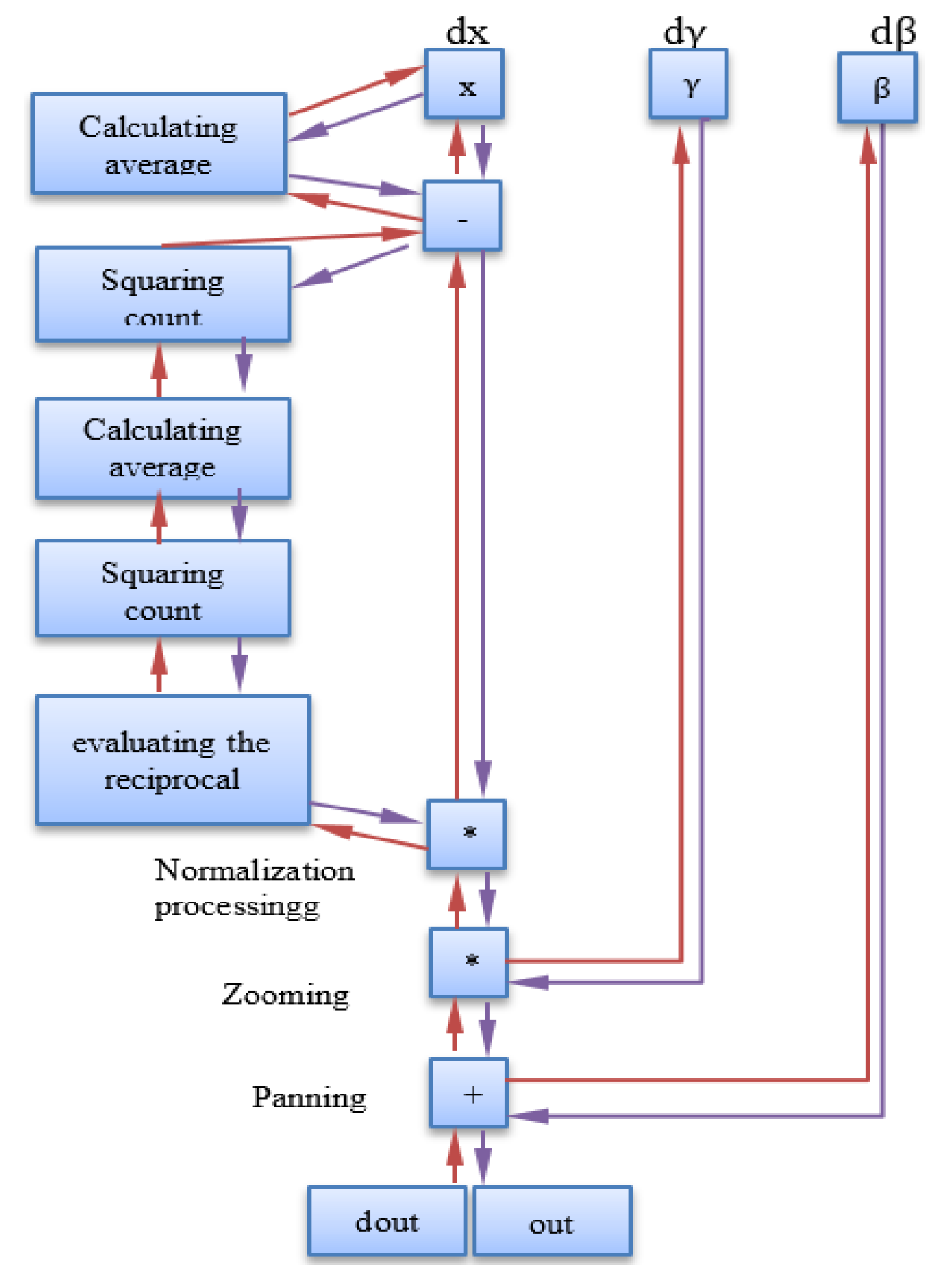
The flow chart is given in Figure 10.
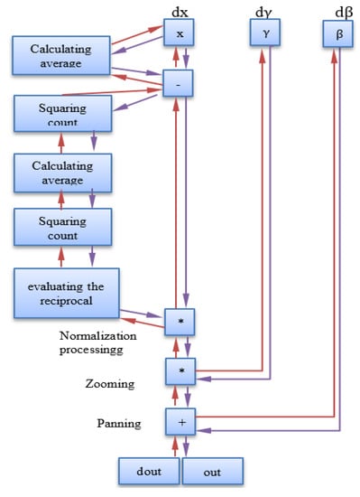
Figure 10.
Calculation diagram of BatchNorm Layer.
The average value of each dimension in the feature space is calculated from the input, and then the average value vector is subtracted from each training sample. After this operation is completed, the variance of each dimension is calculated after the lower branch, and the whole denominator of the normalization equation is calculated. Next, invert it and multiply it by the difference between the input and the mean. The last two operations on the right perform compression by multiplying the input γ and finally adding β to obtain the batch standardized output. When BN is not used, the conversion of the active layer is:
where is the layer input, the weight matrix and the offset vector are the learning parameters of the model, and are nonlinear sigmoid functions. For the sigmoid activation function, the change of at both ends of the function image is small relative to the change of , which is particularly prone to the problem of gradient attenuation. Therefore, some normalization processing before the sigmoid function can alleviate the problem of gradient attenuation. The BN transform is added immediately before the nonlinearity. Since may be another nonlinear output, the shape of its distribution may change during training, and as constraining its first and second moments will not eliminate the covariate shift, we can also normalize the layer input . In contrast, is more likely to have a symmetric non sparse distribution, and normalizing it may produce activation with a stable distribution. The is normalized and the deviation is not taken into account. The effect will be canceled by the subsequent average subtraction. Therefore, is replaced by .
The methods in this paper are compared with other methods, and the results are presented in Table 9.

Table 9.
Comparison of different regularization methods.
By comparing the initial and batch-standardized variants, the number of training steps required to achieve the initial maximum accuracy (72.2%) and the maximum accuracy achieved by network work, it can be found that the BN sigmoid method in this experiment has obtained better results.
In summary, in order to reduce the problem of internal covariate offset, a standardized “layer” must be added before each layer is activated. Each dimension (input neuron) must be standardized separately, instead of being completely consistent with all dimensions. In this way, it is possible to optimize with a higher learning rate without having to accommodate small-scale dimensions as before. Normalization before sigmoid activation function can alleviate the problem of gradient attenuation and achieve better accuracy, and more weight interfaces fall in the data, reducing the risk of overfitting.
3.3. Learning Process
The main network framework Cu net is mainly outlined in Section 3.2. This paper also uses the design principles of Zhang [42] and Zhang [43]. The network composes of 10 convolution blocks conv1-10. The principal coloring network generates training data by converting the color map into a gray map. The conversion of an RGB color image into a gray-scale image is performed by calculating the equivalent gray-scale or the brightness value of each RGB pixel. In the simplest case, L can be taken as the average value of R, G, and B:
In fact, red and yellow look brighter than blue, which causes the red and yellow areas of the image to be darker and the blue areas to be brighter. Therefore, we apply the weighted sum of the color components to calculate the equivalent luminance value.
where .
The input image of the system is , where H and W are the image size. And the input tensor U, the grayscale image is L and the luminance is in the CIE L*a*b*color space. In order to predict the color distribution, the objective of this paper is to learn two AB related color channels . That is, the estimation of the AB color channel of the image. We use CU-net to minimize the objective function. The loss function describes how close the network output is to the color of the real picture.
where D represents the data set.
The loss function is evaluated at each pixel and added together to evaluate the loss of the entire image:
The pixel level Euclidean loss L2 is calculated as follows:
The global cue network and the local cue network are trained as auxiliary networks. During the training, prompts are generated by providing “peeping” or projection of real colors to the network by using functions and , respectively. The expressions input by the user are statistically generated by using functions and as follows:
3.4. CIE L*a*b*color Space
In this paper, we leverage the parameterization of L*a*b*color space by Yan and Zhang et al. [43] in 2016 to divide the AB space into 10 × 10 bins and q = 313 bins kept within the color gamut. The L*a*b*color model linearizes the color representation according to people’s perception of color, and creates a more intuitive coloring system. The dimension of the color space includes luminance L and two color components a and b, where a and b determine the hue and saturation of the color along the green-red and blue-yellow axes, respectively. Compared with RGB, the range of L*a*b*color space is very different. The value range of chromate-graphic ab in L*a*b* is [−128, 128]. If all the values of the output layer are divided by 128, its range becomes [−1, 1]. In order to map these values, the tanh activation function is used at the last layer of the convolutional neural network, because the input of the tanh function can be any value and the output is [−1, 1], and the two can be matched.
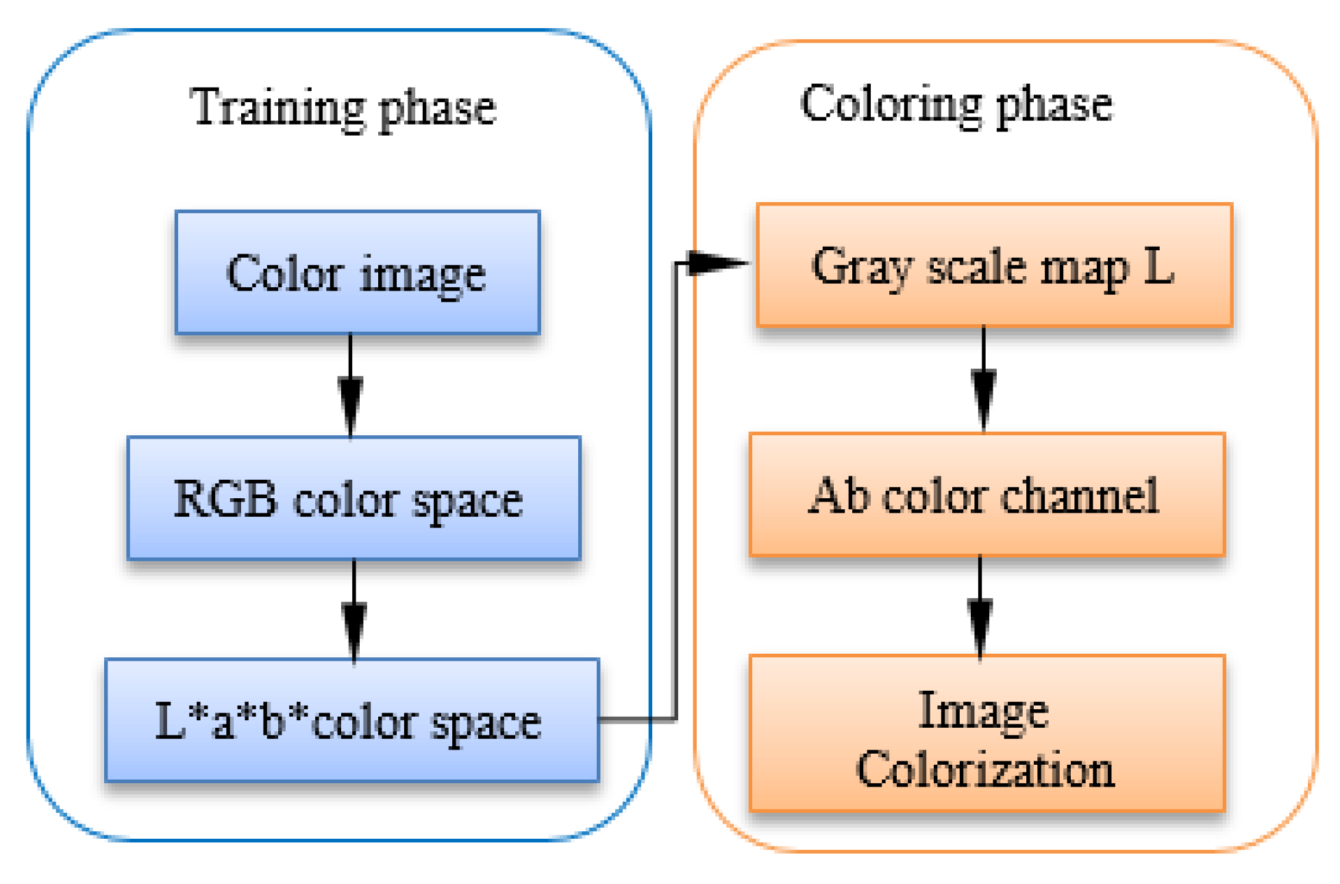
The final prediction is as follows: we input the gray level (L) to the network, and then predict the two color layers ab in L*a*b*color space. To create the final output color image, we need to superimpose the input gray level (L) image and the output layers a and b to create an L*a*b*image. The specific process is shown in Figure 11.
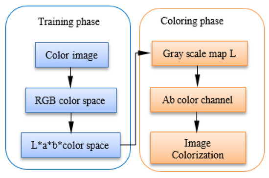
Figure 11.
Color space conversion flow chart of color map generation. The training phase is shown in blue; the coloring phase is represented in orange.
4. Experimental Results
In this section, experiments were implemented using MATLAB 2019a on a personal computer with an Intel® Core i7-4790 CPU @ 3.60 GHz, 16 GB RAM, to demonstrate the efficacy of the proposed scheme.
4.1. Calculate Color Histogram
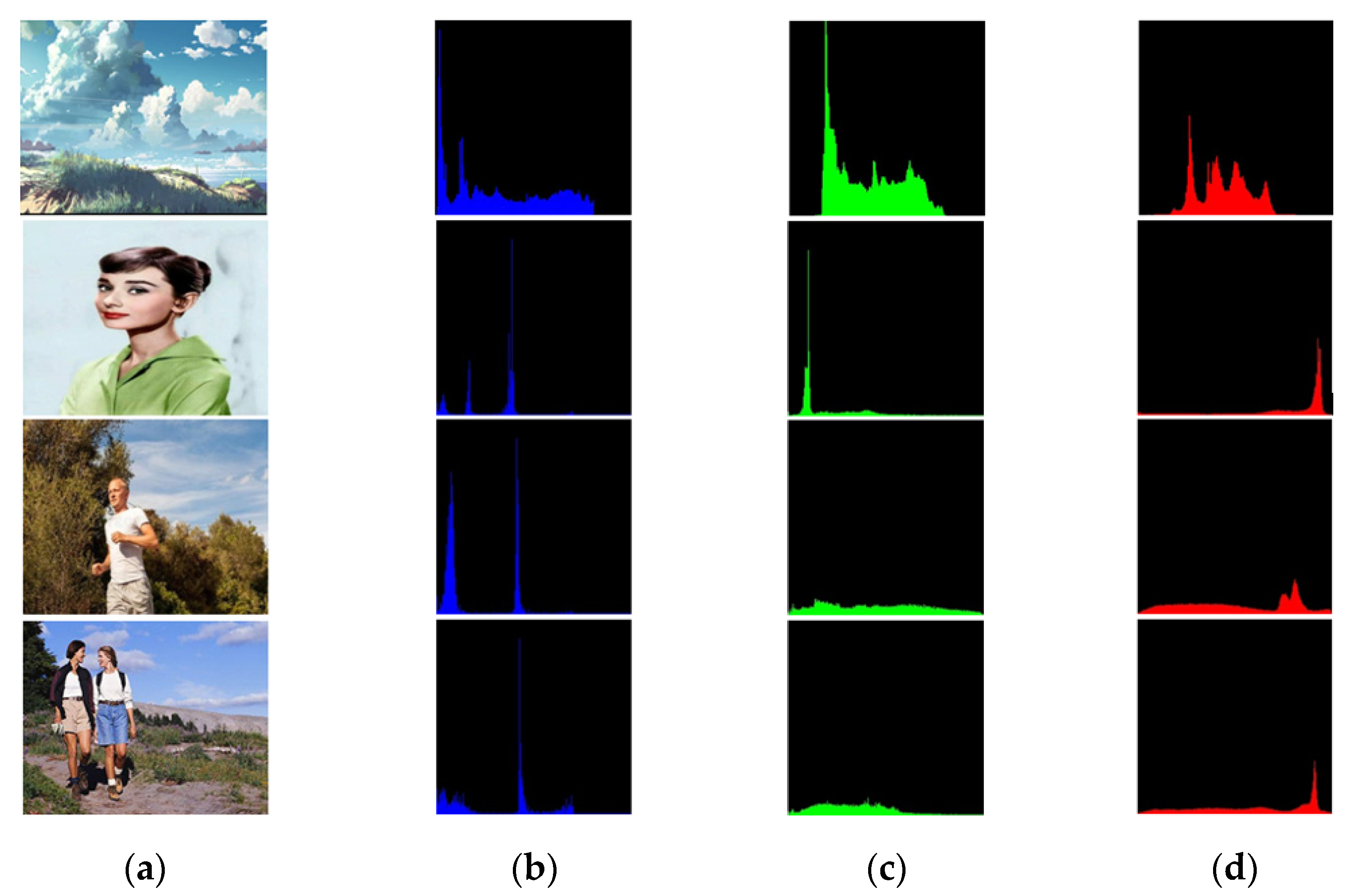
In image processing, the color histogram represents the distribution of colors in an image. For digital images, the color histogram represents the number of pixels with colors in each fixed color range list in the color space of the image, which spans the color space of the image, that is, the set of all possible colors. When we calculate the pixels of different colors in an image, we can first divide the color space into a certain number of small intervals, each interval is called bin, and this process is called color quantization. Then the color histogram of the image is achieved by calculating the number of pixels in each interval. It displays different types of colors in the picture and calculates the number of pixels for each color.
Acquiring the color histogram can determine the color characteristics expressed by the image to a certain extent, and can also be employed to determine the approximate type of the depicted scene or estimate the similarity between images. A histogram is a vector whose component represents a count of the number of pixels having similar colors in an image. Thus, the color histogram can be viewed as a marker extracted from the complete image. Color histograms extracted from different images are indexed and stored in a neural network. During the retrieval, the Euclidean distance is designed to compare the histogram of the query image with the histogram of the neural network training image, so as to give an appropriate coloring effect. Since the color histogram is the global feature of an image, the method based on the color histogram is invariant to translation and rotation, and changes with normalization. Figure 12 illustrates the color histograms. It can be seen that the histogram of the first picture is very different from the last three pictures, because the first type is a landscape map, and the last three pictures are all pictures containing people. The histograms of the third and fourth images are particularly similar, because they all include the sky, green plants and people, while the second image has only one person, so there are differences in hue and saturation. Figure 12 illustrates the color space conversion flow chart of color map generation.

Figure 12.
Color space conversion flow chart of color map generation. The training phase is presented in blue; the coloring phase is represented in orange. (a) Original figure; (b) H channel; (c) S channel; (d) V channel.
Next, the Euclidean distance is utilized to calculate the difference of histogram, and then the matching image is obtained. Let , , and denote the number of elements of the image matrix. In the n-dimensional space, two image matrices and each form a point. Then, the distance between the two points is measured by using the Euclidean distance formula. The smallest distance is the most matching image. The Euclidean distance formula is:
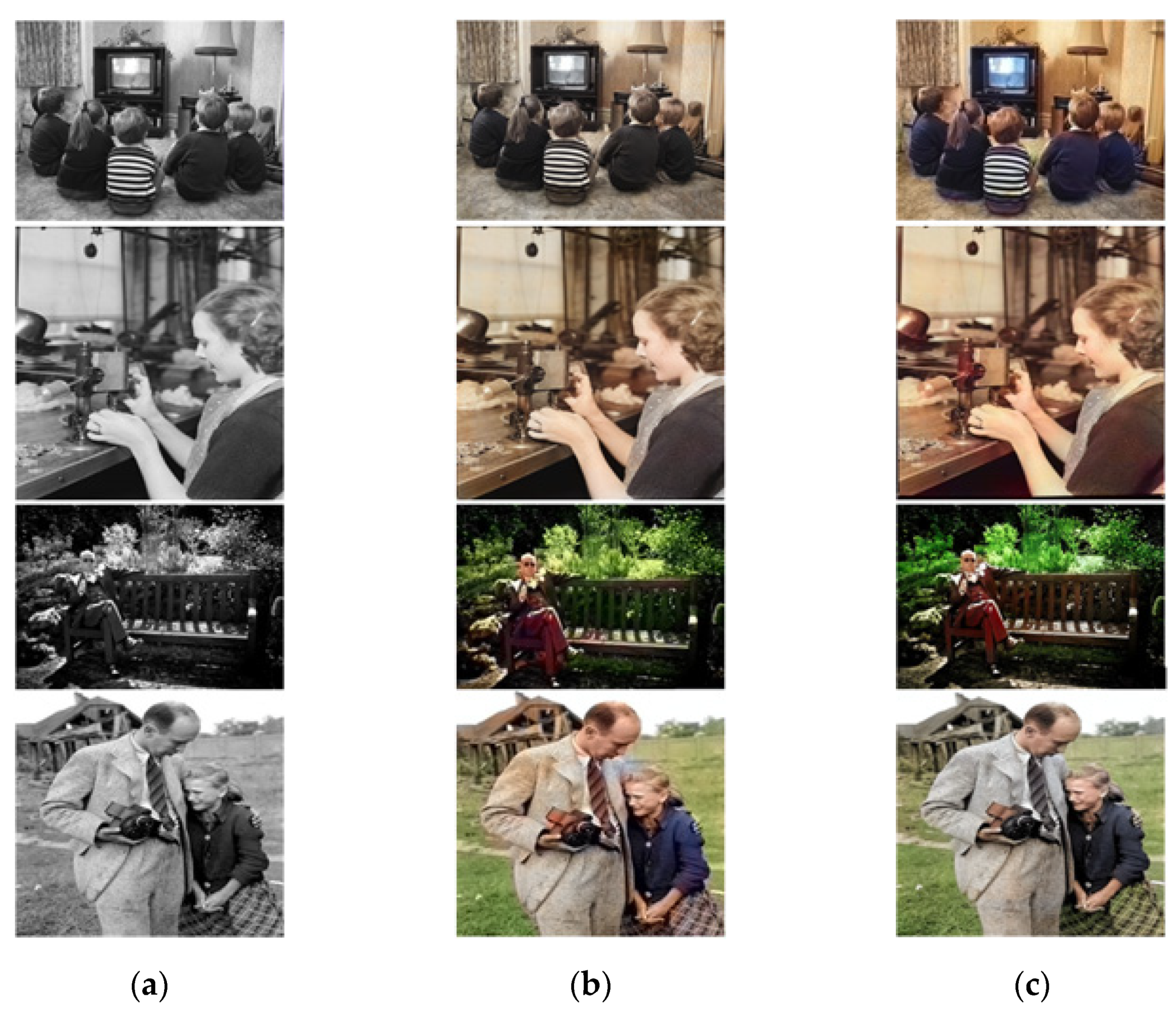
is the distance between the points in the two multidimensional spaces and . Then we color the character image reasonably according to the color histogram obtained. Similarly, we obtain the color histogram of one image and then transfer it to another image. The coloring effect is illustrated in Figure 13c. It can be observed in from Figure 13 that the coloring effect of the indoor image is completely different from that of the outdoor. The indoor color is relatively warm. Much furniture is brown or light brown, while the outdoor color is vibrant green, which is the color of nature. After coloring the black-and-white images, people can truly feel the atmosphere of the image scene. This paper also compares with the method of Yan et al. [34]. Figure 13b demonstrates that this paper has an accurate boundary discrimination effect, regardless of whether it is an individual or a background, and color crossing rarely occurs. In addition, the background coloring is more realistic. For example, the leaves are greener and more realistic.
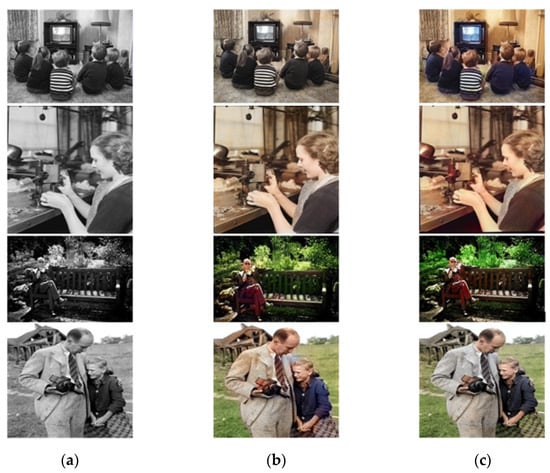
Figure 13.
Global histogram contrast coloring. (a) Gray scale map; (b) Yan et al. [34]; (c) Proposed.
4.2. Qualitative Comparison
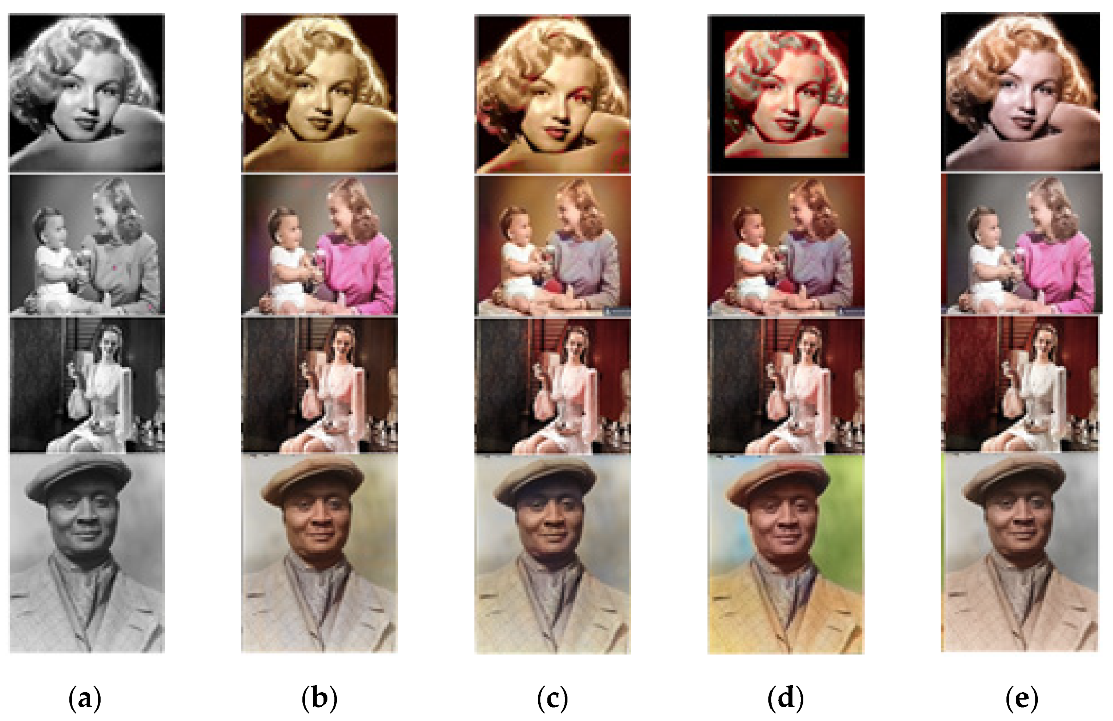
In the following, the coloring effect of this paper is compared with several other coloring effects. It can be seen that the networks and algorithms used in this paper are better than other coloring networks as a whole. They perform well in terms of the realism of the face, the boundary of the coloring, and the control of the background. The effect comparison is presented in Figure 14.

Figure 14.
Qualitative comparison of different image colorization algorithm. (a) Gray scale map; (b) Zhang et al. [42]; (c) Larsson et al. [35]; (d) Endo et al. [44]; (e) Proposed.
It can be seen from Figure 14 that the method in this paper is better than other methods in controlling the color of the background and the characters, and there is no coloring beyond the boundary. Moreover, it is more realistic in the skin color of the characters, and the color of the clothes is bright, and there is no fuzzy boundary and exaggerated color effect.
4.3. Evaluation Criterion
The evaluation of image processing results is a very important part of image processing. In order to measure the image quality after processing, PSNR (Peak Signal to Noise Ratio) value is usually used to measure whether the processing is satisfactory. The PSNR can be defined by mean square error (MSE) [45].
The PSNR is defined by:
where represents the denoised pixel, represents the input pixel with impulse noise, and and represent the length and width of the image, respectively. Generally, the higher the PSNR is, the better the quality of the image. This paper also uses this standard to evaluate the image effect after coloring. Table 10 shows the comparison between the method used in this paper and other coloring methods.

Table 10.
PSNR values of various methods.
5. Conclusions and Future Directions
Image colorization is a challenging task in the field of image processing, which has a wide range of applications in various fields. With the continuous improvement of deep learning network and the updating and iteration of computer hardware equipment, more and more scholars try to apply deep learning methods to the field of image processing. In this paper, several common deep learning methods of image processing are introduced, and the disadvantages of these methods are briefly summarized. In this paper, the U-net network is selected for improvement as the main network structure of coloring. The four down-sampling and four up-sampling processes of the original network are changed to three times to reduce the depth of the network and perform semantic segmentation. The sigmoid activation function is used instead of ReLu, and we place the batch normalization before each activation function to accelerate the training of the network and to improve the accuracy. The extended convolution is introduced to expand the receptive field of the original network without losing the spatial resolution of the image. Then, the lab color space is used as the color space of the colorization task, and the Euclidean distance is calculated. Finally, the reasonable coloring is carried out according to the similarity of the color histogram to obtain a better feature map.
This paper focuses on the methods of generating various coloring effects from human images, and has achieved satisfactory results. However, there are still shortcomings, which need to be improved and perfected continuously. In the future work, it is considered to conduct experiments on higher performance computers to improve the training speed. When we established the main network, many parameters in the improved U-net algorithm were obtained under the condition of experiments. Compared with other neural networks, the network layer might be slightly shallow, which would also limit the training results of the network. In the future, more experimental studies will be performed on the network structure to obtain better network models and coloring results.
Author Contributions
G.-D.C. conceived and designed the experiments; N.W. performed the experiments and wrote the paper; Y.T. analyzed the data and reviewed the paper. All authors have read and agreed to the published version of the manuscript.
Funding
This work was supported in part by the Natural Science Foundation of Fujian Province under Grant No. 2020J01302, which was sponsored by Fujian Provincial Science and Technology Department.
Conflicts of Interest
The authors declare no conflict of interest.
References
- Gupta, R.K.; Chia, Y.S.; Rajan, D.; Ng, E.S.; Huang, Z.Y. Image colorization using similar images. In Proceedings of the 20th ACM International Conference on Multimedia, Nara, Japan, 29 October–2 November 2012; pp. 369–378. [Google Scholar]
- Long, J.; Feng, X.; Zhu, X.; Zhang, J.; Gou, G. Efficient Superpixel-Guided Interactive Image Segmentation Based on Graph Theory. Symmetry 2018, 10, 169. [Google Scholar] [CrossRef]
- Fier, J.; Jamrika, O.; Luká, M.; Shechtman, E.; Asente, P.; Lu, J.; Sykora, D. StyLit: Illumination-Guided Example-Based Stylization of 3D Renderings. ACM Trans. Graph. 2016, 35, 92.1–92.11. [Google Scholar] [CrossRef]
- Al-Rousan, R.; Sunar, M.S.; Kolivand, H. Interactive toon shading using mesh smoothing. Int. J. Intell. Syst. Technol. Appl. 2016, 15, 218–229. [Google Scholar] [CrossRef]
- Ramos, S.; Trevisan, D.F.; Batagelo, H.C.; Sousa, M.C.; Gois, J.P. Contour-Aware 3D Reconstruction of Side-View Sketches. Comput. Graph. 2018, 77, 97–107. [Google Scholar] [CrossRef]
- Wada, T. Automatic colorization of near-infrared monochrome face image based on pixel-wise classification and regression. Tech. Rep. Ieice Multimed. Virtual Environ. 2012, 112, 353–358. [Google Scholar]
- Iizuka, S.; Simo-Serra, E.; Ishikawa, H. Let there be color!: Joint end-to-end learning of global and local image priors for automatic image colorization with simultaneous classification. ACM. Trans. Graph. 2016, 35, 1–11. [Google Scholar] [CrossRef]
- Liu, X.H.; Zou, Y.; Kuang, H.L.; Ma, X.L. Face Image Age Estimation Based on Data Augmentation and Lightweight Convolutional Neural Network. Symmetry 2020, 12, 146. [Google Scholar] [CrossRef]
- Zheng, Y.X.; Liu, R.Q.; Wang, Z.Z.; Wang, S.W.; Zhu, J.C. Detection of Key Points in Mice at Different Scales via Convolutional Neural Network. Symmetry 2022, 14, 1437. [Google Scholar] [CrossRef]
- Thakur, N.; Han, C.Y. Multimodal Approaches for Indoor Localization for Ambient Assisted Living in Smart Homes. Information 2021, 12, 114. [Google Scholar] [CrossRef]
- Rahimi, I.; Gandomi, A.H.; Asteris, P.G.; Chen, F. Analysis and Prediction of COVID-19 Using SIR, SEIQR, and Machine Learning Models: Australia, Italy, and UK Cases. Information 2021, 12, 109. [Google Scholar] [CrossRef]
- Cheng, Z.; Yang, Q.; Sheng, B. Deep colorization. In Proceedings of the International Conference on Computer Vision, Santiago, Chile, 7–13 December 2015; pp. 415–423. [Google Scholar]
- Tola, E.; Lepetit, V.; Fua, P. Daisy: An efficient dense descriptor applied to wide-baseline stereo. IEEE. Trans. Pattern Anal. Mach. Intell. 2009, 32, 815–830. [Google Scholar] [CrossRef]
- Cao, Y.; Zhou, Z.; Zhang, W.; Yu, Y. Unsupervised diverse colorization via generative adversarial networks. In Proceedings of the Joint European Conference on Machine Learning and Knowledge Discovery in Databases, Skopje, Macedonia, 18–22 September 2017; pp. 151–166. [Google Scholar]
- Liu, Y.; Qin, Z.; Wan, T.; Luo, Z. Auto-painter: Cartoon image generation from sketch by using conditional Wasserstein generative adversarial networks. Neurocomputing 2018, 311, 78–87. [Google Scholar] [CrossRef]
- Guadarrama, S.; Dahl, R.; Bieber, D.; Norouzi, M.; Shlens, J.; Murphy, K. PixColor: Pixel Recursive Colorization. In Proceedings of the British Machine Vision Conference, London, UK, 4–7 September 2017; pp. 1–17. [Google Scholar]
- Su, J.W.; Chu, H.K.; Huang, J.B. Instance-Aware Image Colorization. In Proceedings of the Conference on Computer Vision and Pattern Recognition, Seattle, WA, USA, 14–19 June 2020; pp. 7965–7974. [Google Scholar]
- Patricia, V.; Lara, R.; Coloma, B. ChromaGAN: Adversarial Picture Colorization with Semantic Class Distribution. In Proceedings of the Winter Conference on Applications of Computer Vision, Snowmass Village, CO, USA, 2–5 March 2020; pp. 2435–2443. [Google Scholar]
- Gao, Y.; Ding, Y.; Wang, F.; Liang, H. Attentional colorization networks with adaptive group-instance normalization. Information 2020, 11, 479. [Google Scholar] [CrossRef]
- Li, G.; Xu, W. Process weather image by some CNN. In Proceedings of the World Automation Congress, Puerto Vallarta, Mexico, 24–28 June 2012; pp. 1–6. [Google Scholar]
- D’Haro, L.F.; Banchs, R.E.; Chan, K.L.; Daven, L.G.M.; Yuan, N.T. Automatic labelling of touristic pictures using CNNs and metadata information. In Proceedings of the IEEE conference on Signal & Image Processing, Nanyang, Singapore, 4–6 August 2017; pp. 65–73. [Google Scholar]
- Levin, A.; Lischinski, D.; Weiss, Y. Colorization using optimization. ACM. Trans. Graph. 2004, 23, 689–694. [Google Scholar] [CrossRef]
- Yatziv, L.; Sapiro, G. Fast image and video colorization using chrominance blending. IEEE Trans. Image Process. 2006, 15, 1120–1129. [Google Scholar] [CrossRef]
- Sangkloy, P.; Lu, J.W.; Fang, C.; Yu, F.; Hays, J. Scribbler: Controlling Deep Image Synthesis with Sketch and Color. In Proceedings of the 2017 International conference on Computer Vision and Pattern Recognition (CVPR), Honolulu, HI, USA, 22–25 July 2017; pp. 6836–6845. [Google Scholar]
- Reinhard, E.; Ashikhmin, M.; Gooch, B.; Shirley, P. Color transfer between images. IEEE Comput. Graph. Appl. 2002, 21, 34–41. [Google Scholar] [CrossRef]
- Welsh, T.; Ashikhmin, M.; Mueller, K. Transferring Color to Greyscale Images. ACM Trans. Graph. 2002, 21, 277–280. [Google Scholar] [CrossRef]
- Xiang, Y.; Zou, B.; Li, H. Selective color transfer with multi-source images. Pattern Recognit. Lett. 2009, 30, 682–689. [Google Scholar] [CrossRef]
- Ironi, R.; Cohen-Or, D.; Lischinski, D. Colorization by Example. In Proceedings of the Sixteenth Eurographics Conference on Rendering Techniques (DBLP), Konstanz, Germany, 29 June–1 July 2005; pp. 201–210. [Google Scholar]
- Chia, Y.S.; Zhuo, S.; Gupta, R.K.; Tai, Y.W.; Cho, S.Y.; Ping, T.; Lin, S. Semantic colorization with internet images. In Proceedings of the 2011 SIGGRAPH Asia Conference, Hong Kong, China, 12–15 December 2011; pp. 156.1–156.7. [Google Scholar]
- Rizzi, A.; Gatta, C.; Marini, D. A new algorithm for unsupervised global and local color correction. Pattern Recognit. Lett. 2003, 24, 1663–1677. [Google Scholar] [CrossRef]
- Morimoto, Y.; Taguchi, Y.; Naemura, T. Automatic colorization of grayscale images using multiple images on the web. In Proceedings of the International Conference on Computer Graphics and Interactive Techniques, New Orleans, LA, USA, 3–7 August 2009; p. 59. [Google Scholar]
- Cohen-Or, D.; Sorkine, O.; Gal, R.; Leyvand, T.; Xu, Y.Q. Colorharmonization. ACM Trans. Graph. 2006, 25, 624–630. [Google Scholar] [CrossRef]
- Bychkovsky, V.; Paris, S.; Chan, E.; Durand, F. Learning photographic global tonal adjustment with a database of input/output image pairs. In Proceedings of the 2011 International Conference on Computer Vision and Pattern Recognition (CVPR), Colorado, CO, USA, 20–25 June 2011; pp. 97–104. [Google Scholar]
- Yan, Z.C.; Zhang, H.; Wang, B.Y.; Paris, S.; Yu, Y.Z. Auto-matic Photo Adjustment Using Deep Neural Networks. ACM Trans. Graph. 2016, 35, 1–15. [Google Scholar] [CrossRef]
- Larsson, G.; Maire, M.; Shakhnarovich, G. Learning Representations for Automatic Colorization. In Proceedings of the European Conference on Computer Vision 2016, Amsterdam, The Netherlands, 8–16 October 2016; pp. 577–593. [Google Scholar]
- Qin, P.; Cheng, Z.; Cui, Y.; Zhang, J.; Miao, Q. Research on Image Colorization Algorithm Based on Residual Neural Network. In Proceedings of the CCF Chinese Conference on Computer Vision, Tianjin, China, 11–14 October 2017; pp. 608–621. [Google Scholar]
- Russakovsky, O.; Deng, J.; Su, H.; Krause, J.; Satheesh, S.; Ma, S.; Huang, Z.; Karpathy, A.; Khosla, A.; Bernstein, M.; et al. ImageNet Large Scale Visual Recognition Challenge. Comput. Vis. 2015, 115, 211–252. [Google Scholar] [CrossRef]
- Ronneberger, O.; Fischer, P.; Brox, T. U-Net: Convolutional networks for biomedical image segmentation. In Proceedings of the International Conference on Medical image computing and computer Assisted Interventions, Munich, Germany, 5–9 October 2015; pp. 234–241. [Google Scholar]
- Beeche, C.; Singh, J.P.; Leader, J.K.; Gezer, N.S.; Oruwari, A.P.; Dansingani, K.K.; Chhablani, J.; Pu, J. Super U-Net: A modularized generalizable architecture. Pattern Recognit. 2022, 128, 1–12. [Google Scholar] [CrossRef]
- Zhang, X.; Zou, Y.; Wei, S. Dilated convolution neural network with LeakyReLU for environmental sound classification. In Proceedings of the IEEE Conference on Digital Signal Processing, London, UK, 23–25 August 2017; pp. 2165–3577. [Google Scholar]
- Ioffe, S.; Szegedy, C. Batch normalization: Accelerating deep network training by reducing internal covariate shift. In Proceedings of the 32nd International Conference on International Conference on Machine Learning, Lille, France, 6–11 July 2015; pp. 448–456. [Google Scholar]
- Zhang, R.; Isola, P.; Efros, A.A. Colorful Image Colorization. In Proceedings of the European Conference on Computer Vision 2016, Amsterdam, The Netherlands, 8–16 October 2016; pp. 649–666. [Google Scholar]
- Zhang, R.; Zhu, J.Y.; Isola, P.; Geng, X.; Lin, A.S.; Yu, T.H.; Efros, A.A. Real-time user-guided image colorization with learned deep priors. ACM. Trans. Graphics. 2017, 36, 1–11. [Google Scholar] [CrossRef]
- Endo, Y.; Iizuka, S.; Kanamori, Y.; Mitani, J. Deepprop: Extracting deep features from a single image for edit propagation. Comput. Graph. Forum. 2016, 35, 189–201. [Google Scholar] [CrossRef]
- Guo, S.; Wang, G.; Han, L.; Song, X.; Yang, W. COVID-19 ct image denoising algorithm based on adaptive threshold and optimized weighted median filter. Biomed. Signal Process. Control 2022, 75, 103552. [Google Scholar] [CrossRef]
Publisher’s Note: MDPI stays neutral with regard to jurisdictional claims in published maps and institutional affiliations. |
© 2022 by the authors. Licensee MDPI, Basel, Switzerland. This article is an open access article distributed under the terms and conditions of the Creative Commons Attribution (CC BY) license (https://creativecommons.org/licenses/by/4.0/).


