
Mapping Properties of Associate Laguerre Polynomials in Leminiscate, Exponential and Nephroid Domain


Department of Mathematics and Statistics, College of Science, King Faisal University, Al-Hasa 31982, Saudi Arabia
Symmetry 2022, 14(11), 2303; https://doi.org/10.3390/sym14112303
Submission received: 21 September 2022
/
Revised: 19 October 2022
/
Accepted: 20 October 2022
/
Published: 3 November 2022
(This article belongs to the Special Issue Symmetries of Difference Equations, Special Functions and Orthogonal Polynomials)
Abstract
:The function maps the unit disc to a leminscate which is symmetric about the x-axis. The conditions on the parameters and n, for which the associated Laguerre polynomial (ALP) maps unit disc into the leminscate domain, are deduced in this article. We also establish the condition under which a function involving maps to a domain subordinated by , , and , . We provide several graphical presentations for a clear view of some of the obtained results. The possibilities for the improvements of the results are also highlighted.
MSC:
30C10; 30C451. Introduction
The generalized [1] or associated Laguerre polynomial (ALP) is the solution of the differential equation
which is represented by the series
where is the confluent hypergeometric function, and is the well-known Pochhammer symbol defined as
The first few terms of the polynomial are given as
ALP has its own significance in various branches of mathematics and physics and has a wide contribution in different aspects in mathematical research. The associated Laguerre polynomials are orthogonal with respect to the gamma distribution on the interval . The generalized Laguerre polynomials are widely used in many problems of quantum mechanics, mathematical physics and engineering. In quantum mechanics, the Schrödinger equation for the hydrogen-like atom is exactly solvable by separation of variables in spherical coordinates, and the radial part of the wave function is an ALP [2]. In mathematical physics, vibronic transitions in the Franck–Condon approximation can also be described by using Laguerre polynomials [3]. In engineering, the wave equation is solved for the time domain electric field integral equation for arbitrary shaped conducting structures by expressing the transient behaviors in terms of Laguerre polynomials [4]. The monographs by Szegó [5], and Andrews, Askey, and Roy [6] include a wealth of information about ALP and other orthogonal polynomial families.
In this study, we consider
The function satisfies the normalization condition and is a solution of the differential equation
The following four functions are also important for this study.
The function maps to a leminscate, shifted to a disc center at with radius , maps to the exponential domain, and maps to the neuphroid domain as shown in Figure 1.
Let denote the class of functions in the open unit disk and normalized by the conditions . If f and g are analytic in , then f is subordinate to g, written or if there is an analytic self-map of satisfying and , . Especially, if is univalent in , then if and only if and . It is worth noting here that , , and are not subordinate to each other as it is clear from Figure 1 that the image of by any one of these functions does not contain the image by others. Differential subordination is an important technique to study geometric functions theory. Details about this technique can be seen in [7,8].
Denote by and , respectively the important subclasses of consisting of univalent starlike and convex functions. Geometrically, if the linear segment , lies completely in whenever , while if is a convex domain. Related to these subclasses is the Cárathèodory class consisting of analytic functions p satisfying and in . Analytically, if , while if . It is well-known that the function is starlike and is convex in the unit disk .
A function is lemniscate convex if lies in the region bounded by right half of lemniscate of Bernoulli given by , which is equivalent to the subordination . Similarly, the function f is lemniscate starlike if . On the other hand, the function is lemniscate Carathéodory if . Clearly, a lemniscate Carathéodory function is a Carathéodory function and hence is univalent.
The sufficient conditions of starlikeness associated with lemniscate of Bernoulli are obtained in [9]. A similar study associated with the exponential domain is conducted in [10]. One of the motivations of this work is the nephroid curve
Recently, the nephroid curve received attention of researchers in geometric functions theory thanks to the work by Wani and Swaminathan [11,12,13]. This two-cusped kidney-shaped curve was first studied by Huygens and Tschirnhausen in 1697. However, the word nephroid was first used by Richard A. Proctor in 1878 in his book The Geometry of Cycloids. For further details related to the nephroid curve, we refer to [11,14]. The radius of starlikeness and convexity for functions associated with the nephroid domain is discussed in [13]. In [12], the authors discuss the starlike and convex functions associated with the nephroid domain. The Fekete–Szegö kind of inequalities for certain subclasses of analytic functions in association with the nephroid domain is studied in [15].
Significant findings from the articles [9,10] are summarized, respectively, in Lemma 1 and Lemma 2, while Lemma 3 and Lemma 4 highlights the results from the reference [11]. The special functions, such as Bessel, Struve, Confluent hypergeometric and hypergeometric, are closely associated with the geometric functions theory. The geometric nature of these special functions associated with the leminisciate, the exponential and the nephroid domain are studied in [9,10,13]. The lemniscate convexity of generalized Bessel functions is studied in [9], while [10] deals with the exponential starlikeness and convexity of confluent hypergeometric, Lommel and Struve functions.
In this paper, motivated by the aforementioned works, we investigated the inclusion properties of the normalized function involving ALP that maps the unit disc into the lemniscate and the exponential domain, respectively, in Section 2 and Section 3. Section 4 deals with the results concerning the shifted disc , for . In Section 5, we derive the conditions under which integration associated with maps into the nephroid domain. All the results are interpreted graphically. Several options for the improvement are highlighted.
2. Mapping in the Lemniscate Domain
In this section, we derive the relation between and n for which maps into . To prove the main results related with the lemniscate, the following Lemma 1 is used.
Lemma 1
In the case of two dimensions, if satisfy whenever and for , ,
If for , then in .
Now we state and prove the main result for this section.
Theorem 1.
For , .
Proof.
Let . Suppose that . Define
A natural question arises for a fixed : are the values the best possible in Theorem 1? To investigate it, we try to experiment through graphical representation of and . It is worth noting here that when . We present our cases for .
- n = 2
- By Theorem 1, holds for . However, Figure 2 indicates that for real , the subordination property for which follows for where the possible value is any number in the interval .
- n = 3
- As per Theorem 1, in this case is . Figure 3 indicates that for real , the inclusion holds for where the possible value of is any number in the interval .
- n = 4
- The expected value of is , but as per Figure 4, the value of can be lower down to a number in .
3. Mapping in the Exponential Domain
Lemma 2
Now, we state and prove our main result to have the mapping properties in the exponential domain.
Theorem 2.
For , .
Proof.
Let . Suppose that . Then,
Now
provided . □
4. Mapping in Disc Center at and Radius
The function for maps the unit disc to a disc center at and radius A. In this section, we will derive conditions by which
Theorem 3.
For , and , suppose that
Then, .
Proof.
Let and define as
It is clear from (9) that . We shall apply Lemma 1 to show , which implies .
Graphical representation indicates that there is a provision of improvement for a minimum value of for fixed n and A. For example, set and , and suppose that is real. Then, by Theorem 3, if . However, Figure 10 clearly indicates that the result can hold for . This claim can also be valid theoretically. The subordination is equivalent to
which holds for if . In particular, if is a positive real number, and , then holds for
Similarly for , as per Theorem 3, the subordination holds for . In particular, for real and , the subordination is true when . However, a direct proof indicates that the subordination holds when
Clearly, the second condition is better than the first condition (derived from Theorem 3). For example, if is real and , then holds for . The comparison can be seen in Figure 11.
Based on the above facts, we can conclude that for certain special cases, Theorem 3 has a chance for improvement. Now, we state and prove an improved version of Theorem 3.
Theorem 4.
For real and fixed and , suppose that is the largest root of
Then, the subordination holds for all . The result is sharp as is the best lowest value.
Proof.
The subordination is equivalent to
Now, for , it follows
It can be easily verified that for a fixed n, the function is decreasing; hence, the inequality (11) holds for . Here, is the largest root of the equation
This completes the proof. □
5. Connection with the Nephroid Domain
In this section, we observe that or do not always imply . For example, consider the case when and , the polynomial
as shown in Figure 12a. Now define the function
In Figure 12b, we can see that
To state the next result, let us generalize (12) as follows
We also consider the function
We need the following results in sequence.
Lemma 3
([11]). Let be analytic such that . Then, the following subordination implies
- (i)
- for
- (ii)
- for
Lemma 4
([11]). Let be analytic such that . Then the following subordination imply
- (i)
- for ,
- (ii)
- for
- (iii)
- for
- (iv)
- for ,
- (v)
- for
- (vi)
- for
The following subordination holds true.
Theorem 5.
For and , the following subordination holds
- (i)
- for
- (ii)
- for
- (iii)
- for
Proof.
It is worth noting that for , Theorem 2 implies that
Now, it follows from (13) that
The first three cases along with Lemma 4 (part (iv)–(vi)) helps to conclude the result, while the fourth case together with Lemma 3 (part (ii)) implies the result. □
As of a final result, we have the following that can be proved using Theorem 1 and Lemma 4 (part (i)–(iii)) and Lemma 3 (part (i)). We omit the details of the proof.
Theorem 6.
For and , the following subordination holds
- (i)
- for
- (ii)
- for
- (iii)
- for
Now, we are going to interpret the result obtained in Theorem 5 graphically. For this, we consider the special case where . In the case , we set the smallest value of . Now, by judicious choice of n (we chose up to 5000), we can see through Figure 13 that holds. This indicates that in the case for all , the smallest value of is sharp. However, in case of a fixed n, there is a possibility to lower the value of as presented in Table 2.
Clearly is approaching the value for increasing n.
Similar analysis of results can also be computed for part of Theorem 5 ((ii) & (iii)) and Theorem 6. We avoid such details. However, this fact leads to an open problem as stated below
Problem 1
(Open). Find the exact value of for all n, α such that ; ; and holds for .
6. Conclusions
By using results from the articles [9,10], we find the conditions on the parameter and n such that
is starlike in the , , . We also consider two integrals involving , namely
Then, using results from [11], we derive conditions on and n by which the functions and are subordinated by .
Different graphical presentations demonstrate that the findings in this study are valid. However, there is potential for improvement in a few instances. We conclude by emphasizing that the open cases regarding the function which are highlighted in this study are required for some alternative methods in contrast to those found in the references [9,10,11]. This could be an interesting topic for further study.
Funding
This work was supported by the Deanship of Scientific Research, Vice Presidency for Graduate Studies and Scientific Research, King Faisal University, Saudi Arabia [Grant No. 780].
Institutional Review Board Statement
Not applicable.
Informed Consent Statement
Not applicable.
Data Availability Statement
Not applicable.
Conflicts of Interest
The authors declare no conflict of interest.
References
- Abramowitz, M.; Stegun, I.A. A Handbook of Mathematical Functions; John Wiley & Sons, Inc.: New York, NY, USA, 1965. [Google Scholar]
- Mawhin, J.; Ronveaux, A. Schrödinger and Dirac equations for the hydrogen atom, and Laguerre polynomials. Arch. Hist. Exact Sci. 2010, 64, 429–460. [Google Scholar] [CrossRef]
- de Jong, M.; Seijo, L.; Meijerink, A.; Rabouw, F.T. Resolving the ambiguity in the relation between Stokes shift and Huang-Rhys parameter. Phys. Chem. Chem. Phys. 2015, 17, 16959–16969. [Google Scholar] [CrossRef] [PubMed] [Green Version]
- Chung, Y.-S.; Sarkar, T.K.; Jung, B.H.; Salazar-Palma, M.; Ji, Z.; Jang, S.; Kim, K. Solution of time domain electric field integral equation using the Laguerre polynomials. IEEE Trans. Antennas Propag. 2004, 52, 2319–2328. [Google Scholar] [CrossRef]
- Szegö, G. Orthogonal Polynomials; American Mathematical Society Colloquium Publications; American Mathematical Society: New York, NY, USA, 1939; Volume 23. [Google Scholar]
- Andrews, G.E.; Askey, R.; Roy, R. Special Functions; Encyclopedia of Mathematics and its Applications, 71; Cambridge University Press: Cambridge, UK, 1999. [Google Scholar]
- Miller, S.S.; Mocanu, P.T. Differential subordinations and inequalities in the complex plane. J. Differ. Equations 1987, 67, 199–211. [Google Scholar] [CrossRef] [Green Version]
- Miller, S.S.; Mocanu, P.T. Differential Subordinations; Monographs and Textbooks in Pure and Applied Mathematics, 225; Dekker: New York, NY, USA, 2000. [Google Scholar]
- Madaan, V.; Kumar, A.; Ravichandran, V. Lemniscate convexity of generalized Bessel functions. Stud. Sci. Math. Hungar. 2019, 56, 404–419. [Google Scholar] [CrossRef]
- Naz, A.; Nagpal, S.; Ravichandran, V. Exponential starlikeness and convexity of confluent hypergeometric, Lommel, and Struve functions. Mediterr. J. Math. 2020, 17, 22. [Google Scholar] [CrossRef]
- Swaminathan, A.; Wani, L.A. Sufficiency for nephroid starlikeness using hypergeometric functions. Math. Methods Appl Sci. 2022, 45, 1–14. [Google Scholar] [CrossRef]
- Wani L., A.; Swaminathan, A. Starlike and convex functions associated with a nephroid domain. Bull. Malays. Math. Sci. Soc. 2021, 44, 79–104. [Google Scholar] [CrossRef]
- Wani, L.A.; Swaminathan, A. Radius problems for functions associated with a nephroid domain. Rev. R. Acad. Cienc. Exactas Fís. Nat. Ser. A Mat. RACSAM 2020, 114, 20. [Google Scholar] [CrossRef]
- Yates, R.C. A Handbook on Curves and Their Properties; Edwards, J.W., Ed.; Literary Licensing, LLC: Ann Arbor, MI, USA, 1947. [Google Scholar]
- Murugusundaramoorthy, G. Fekete–Szegö Inequalities for Certain Subclasses of Analytic Functions Related with Nephroid Domain. J. Contemp. Mathemat. Anal. 2022, 57, 90–101. [Google Scholar] [CrossRef]
- Madaan, V.; Kumar, A.; Ravichandran, V. Starlikeness associated with lemniscate of Bernoulli. Filomat 2019, 33, 1937–1955. [Google Scholar] [CrossRef] [Green Version]
- Naz, A.; Nagpal, S.; Ravichandran, V. Star-likeness associated with the exponential function. Turk. J. Math. 2019, 43, 1353–1371. [Google Scholar] [CrossRef]
Figure 1.
Boundary of , , and .

Figure 2.
Graph of for fixed .

Figure 3.
Graph of for fixed .

Figure 4.
Graph of for fixed .

Figure 5.
Graph of .

Figure 6.
Graph of .
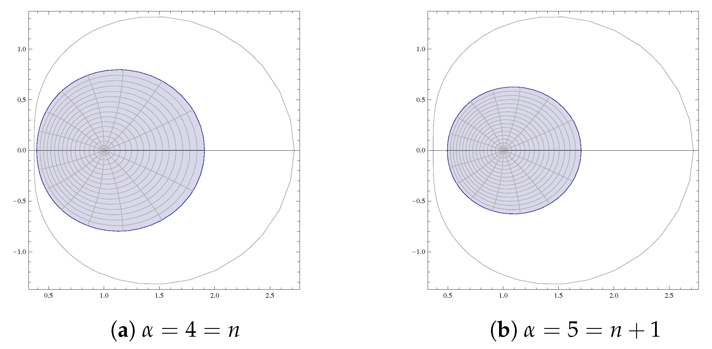
Figure 7.
Graph of .

Figure 8.
Graph of .

Figure 9.
Graph of .

Figure 10.
.

Figure 11.
.
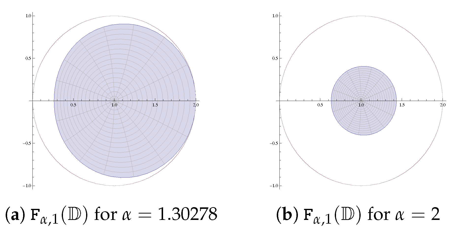
Figure 12.
Comparison of and .

Figure 13.
Graph of .


Table 1.
The value of for fixed A and n.
| n/A | 1 | 2 | 3 | 5 | 10 | 15 |
|---|---|---|---|---|---|---|
| A = 1 | 0 | 1.30278 | 2.67882 | 5.49886 | 12.6531 | 19.8441 |
| A = 1/2 | 1 | 3.37228 | 5.79852 | 10.6945 | 22.9951 | 35.3155 |
| A = 1/3 | 2 | 5.40512 | 8.85262 | 15.7795 | 33.1391 | 50.5122 |
| A = 1/4 | 3 | 7.42443 | 11.8837 | 20.8273 | 43.219 | 65.6208 |
Table 2.
- possible lowest value of for a fixed n.
| n | n | ||
|---|---|---|---|
| 1 | 5 | ||
| 2 | 10 | ||
| 3 | 50 | ||
| 4 | 100 |
Publisher’s Note: MDPI stays neutral with regard to jurisdictional claims in published maps and institutional affiliations. |
© 2022 by the author. Licensee MDPI, Basel, Switzerland. This article is an open access article distributed under the terms and conditions of the Creative Commons Attribution (CC BY) license (https://creativecommons.org/licenses/by/4.0/).
Share and Cite
MDPI and ACS Style
Mondal, S.R. Mapping Properties of Associate Laguerre Polynomials in Leminiscate, Exponential and Nephroid Domain. Symmetry 2022, 14, 2303. https://doi.org/10.3390/sym14112303
AMA Style
Mondal SR. Mapping Properties of Associate Laguerre Polynomials in Leminiscate, Exponential and Nephroid Domain. Symmetry. 2022; 14(11):2303. https://doi.org/10.3390/sym14112303
Chicago/Turabian StyleMondal, Saiful R. 2022. "Mapping Properties of Associate Laguerre Polynomials in Leminiscate, Exponential and Nephroid Domain" Symmetry 14, no. 11: 2303. https://doi.org/10.3390/sym14112303
Note that from the first issue of 2016, this journal uses article numbers instead of page numbers. See further details here.