Analysis of Kink Behaviour of KdV-mKdV Equation under Caputo Fractional Operator with Non-Singular Kernel

Abstract

The KdV equation has many applications in mechanics and wave dynamics. Therefore, researchers are carrying out work to develop and analyze modified and generalized forms of the standard KdV equation. In this paper, we inspect the KdV-mKdV equation, which is a modified and generalized form of the ordinary KdV equation. We use the fractional operator in the Caputo sense to analyze the equation. We examine some theoretical results concerned with the solution’s existence, uniqueness, and stability. We employ a modified Laplace method to extract the numerical results of the considered equation. We use MATLAB-2020 to simulate the results in a few fractional orders. We report the effects of the fractional order on the wave dynamics of the proposed equation.

1. Introduction

In 1895, Korteweg and de Vries proposed a non-linear PDE called the KdV equation, which was used to study the waves that occur on shallow water surfaces. This precisely solvable model has been the subject of numerous studies. Many scholars have suggested novel uses for the production of acoustic waves from ions and crystal lattices in plasma. A standard KdV equation has the form:

$${\mathcal{G}}_t+6\mathcal{G}{\mathcal{G}}_x+{\mathcal{G}}_{xxx}=0.$$

The KdV equation has been applied extensively in a variety of domains, including the understanding of shallow water waves, ion acoustic waves, bubble liquid mixes, and magneto-hydrodynamic waves in warm plasma [1,2]. Specific theoretical physics phenomena connected to quantum mechanics are described using a KdV model. The model is used in the disciplines of fluid dynamics and aerodynamics, continuum mechanics for the creation of shock waves, solitons, turbulence, boundary layer behaviour, and mass transport. It has been studied and used for a long time. Several modifications and generalization forms of the standard KdV equation have been introduced in the literature [3,4,5]. Very recently, Malik et al. [6] introduced a new generalized form of the KdV equation:

$${\mathcal{G}}_{\mathit{t}}=\alpha \mathcal{G}{F}_x-\alpha \mathcal{G}{F}_y+\beta {\mathcal{G}}^2{F}_x-\beta {\mathcal{G}}^2{F}_y+\gamma {\mathcal{G}}_{xxx}-\gamma {\mathcal{G}}_{yyy}-\delta {\mathcal{G}}_{xxy}+\delta {\mathcal{G}}_{xyy},$$

(1)

where $\alpha ,\beta ,\gamma$ and $\delta$ are arbitrary constants. The authors considered some new exact solutions of the proposed KdV equation. This equation has several applications in fluid mechanics and acoustic wave dynamics.

In recent years, non-local operators (NLO) and their applications have become an important research topic for scientists and engineers. NLOs have unique features and advantages that are absent in integer operators. NLOs can provide past information about a physical process. The most well-known and widely used NLO operator is the Caputo operator. This operator has been used for modeling and analyzing many physical events [7,8]. After much time, it was found that the Caputo operator has a singularity issue in the kernel. So, to address this issue, Caputo and his co-author Fabrizio modified the Caputo operator by replacing the power-law kernel by an exponential-decay kernel. The new operator was named the Caputo–Fabrizio (CF) operator. The CF operator has also been applied to the analysis of several phenomena [9,10]. After one year, it was determined that the CF operator possesses a local kernel. Hence, Atangana and Baleanu replaced the exponential decay with a Mittag–Leffler kernel to address the issue of the locality of the kernel in the CF operator. The new operator was referred to as the Atangana–Baleanu (AB) operator. Over the past six years, the AB operator has been extensively used by researchers to study the evolution and behavior of non-linear processes. Some applications of the AB operators in physical sciences are listed in [11,12,13,14,15,16]. Fractional calculus has many applications in mathematical physics. For example, Cao et al. studied symmetric and anti-symmetric solitons of the fractional non-linear Schrödinger equation [17]. Li et al. investigated the existence, bifurcation and stability of two-dimensional optical solitons in the framework of the fractional non-linear Schrödinger equation [18]. Mou et al. analyzed coupled discrete conformable fractional non-linear Schrödinger equations [19]. Chen studied combined optical soliton solutions of a (1+1)-dimensional time fractional resonant cubic-quintic non-linear Schrödinger equation in weakly non-local non-linear media [20]. Fang et al. investigated the discrete fractional soliton dynamics of the fractional Ablowitz–Ladik model [21]. Bo and his co-authors analyzed symmetric and antisymmetric solitons in the fractional non-linear Schrödinger equation with saturable non-linearity and PT-symmetric potential [22]. Some further applications of fractional calculus in mathematical physics can be found in the literature [23,24,25].

Motivated by the above literature, we investigate the considered KdV Equation (1) using the AB operator. We explore some qualitative features, such as the existence, uniqueness, and stability of the solution. We use a hybrid Laplace transform to deduce an approximate solution. We simulate the obtained solution for a few fractional orders to show a new type of soliton solution which has not been studied previously in the literature. The structure of the paper is as follows: Section 2 deals with basic concepts of fractional calculus. Section 3 provides an analysis of the considered equation. Section 4 is devoted to solution of the considered equation. The convergence and stability of the method is described in Section 5. The simulation of the obtained results is provided in Section 6. In Section 7, we present the conclusions.

2. Preliminaries

Here, we define the terms Atangana–Baleanu integral and fractional derivative in relation to the Caputo concept.

Definition 1

([26]). For fractional order $0<\mathrm{d}\le 1$ and $\mathit{F}\in H^1(c,d),$ the left-sided $\mathcal{ABC}$ operator is given as:

$${}^{\mathcal{ABC}}{D}_0^{\mathrm{d}}\mathcal{G}\left(\mathit{t}\right)=\frac{\mathcal{M}\left(\mathrm{d}\right)}{(1-\mathrm{d})}{\int }_0^{\mathit{t}}E\left(\frac{-\mathrm{d}}{\mathrm{d}-1}{\left(\mathrm{d}-{\rm Y}\right)}^{\mathrm{d}}\right){\mathcal{G}}^{\prime }({\rm Y})d{\rm Y},\mathrm{d}>0,$$

where $\mathcal{M}\left(\mathrm{d}\right)$ provides a normalization function with $\mathcal{M}\left(0\right)=\mathcal{M}(1=1)$ and $E_{\mathrm{d}}$ is the Mittag–Leffler function, expressed as

$$E_{\mathrm{d}}\left(\mathit{t}\right)={\sum }_{r=0}^{{}^{\infty }}\frac{{\mathit{t}}^{\mathit{r}}}{\Gamma (r+1)}.$$

Definition 2

([26]). The corresponding fractional integral is given by

$${}^{\mathcal{AB}}{I}_0^{\mathrm{d}}\mathcal{G}\left(\mathit{t}\right)=\frac{1-\mathrm{d}}{\mathcal{M}\left(\mathrm{d}\right)}+\frac{\mathrm{d}}{\mathcal{M}\left(\mathrm{d}\right)\Gamma \left(\mathrm{d}\right)}{\int }_0^{\mathit{t}}{(\mathit{t}-{\rm Y})}^{\mathrm{d}-1}\mathcal{G}({\rm Y})d{\rm Y}.$$

Definition 3

([26]). The Laplace transform of the $\mathcal{ABC}$ fractional derivative of $\mathcal{G}\left(\mathit{t}\right)$ is expressed as

$$\mathcal{L}\left({}^{\mathcal{ABC}}{D}_0^{\mathrm{d}}\mathcal{G}\left(\mathit{t}\right)\right)=\frac{\mathcal{M}\left(\mathrm{d}\right)}{s^{\mathrm{d}}(1-\mathrm{d})+\mathrm{d}}\left[s^{\mathrm{d}}\mathcal{L}\left(\mathcal{G}\left(\mathit{t}\right)\right)-s^{\mathrm{d}-1}\mathcal{G}\left(0\right)\right].$$

3. Analysis of Fractional KdV-mKdV Equation

As discussed in the introduction, the fractional operator provides complete past information for a non-linear process. Motivated by this, we consider the KdV-mKdV Equation (1) under the Mitagg–Leffler fractional operator as:

$${}^{\mathcal{ABC}}{D}_t^{\mathrm{d}}\mathcal{G}=\alpha \mathcal{G}{F}_x-\alpha \mathcal{G}{F}_y+\beta {\mathcal{G}}^2{F}_x-\beta {\mathcal{G}}^2{F}_y+\gamma {\mathcal{G}}_{xxx}-\gamma {\mathcal{G}}_{yyy}-\delta {\mathcal{G}}_{xxy}+\delta {\mathcal{G}}_{xyy}.$$

(2)

Here, we discuss some theoretical results for the considered equation. We extract numerical results using the Laplace transform and the Adomian decomposition method. We present the convergence and stability of the solution.

Existence Theory

In this part, some results concerning the existence and uniqueness of the solution will be derived. For this, let

$$\chi (x,y,\mathit{t};\mathcal{G})=\alpha \mathcal{G}{F}_x-\alpha \mathcal{G}{F}_y+\beta {\mathcal{G}}^2{F}_x-\beta {\mathcal{G}}^2{F}_y+\gamma {\mathcal{G}}_{xxx}-\gamma {\mathcal{G}}_{yyy}-\delta {\mathcal{G}}_{xxy}+\delta {\mathcal{G}}_{xyy}.$$

Then, the above Equation (2) becomes:

$${}^{\mathcal{ABC}}{D}_0^{\mathrm{d}}\mathcal{G}(x,y,\mathit{t})=\chi (x,y,\mathit{t};\mathcal{G}).$$

Applying the $\mathcal{AB}$ integral, we get

$$\mathcal{G}(x,y,\mathit{t})-\mathcal{G}(x,y,0)=\frac{1-\mathrm{d}}{\mathcal{M}\left(\mathrm{d}\right)}\chi (x,y,\mathit{t};\mathcal{G})+\frac{\mathrm{d}}{\mathcal{M}\left(\mathrm{d}\right)\Gamma \left(\mathrm{d}\right)}{\int }_0^{\mathit{t}}{(\mathit{t}-{\rm Y})}^{\mathrm{d}-1}\chi (x,y,{\rm Y};\mathcal{G})d{\rm Y}.$$

First, we verify that the Lipschitz condition holds for the kernel $\chi (x,y,\mathit{t};\mathcal{G}).$ Assume two bounded functions $\mathcal{G}$ and $\mathcal{H},$ so $∥\mathcal{G}∥\le {\lambda }_1,$ and $∥\mathcal{H}∥\le {\lambda }_2$, where ${\lambda }_1,{\lambda }_2>0$ and consider

$$\begin{array}{cc}\hfill & ∥\chi (x,y,\mathit{t};\mathcal{G})-\chi (x,y,\mathit{t};\mathcal{H})∥\hfill \\ \hfill & =∥\alpha \left(\mathcal{G}{F}_x-\mathcal{H}{\mathcal{H}}_x\right)-\alpha \left(\mathcal{G}{F}_y-\mathcal{H}{\mathcal{H}}_y\right)+\beta \left({\mathcal{G}}^2{F}_x-{\mathcal{H}}^2{\mathcal{H}}_x\right)-\beta \left({\mathcal{G}}^2{F}_y-{\mathcal{H}}^2{\mathcal{H}}_y\right)\hfill \\ & +\gamma \left({\mathcal{G}}_{xxx}-{\mathcal{H}}_{xxx}\right)-\gamma \left({\mathcal{G}}_{yyy}-{\mathcal{H}}_{yyy}\right)-\delta \left({\mathcal{G}}_{xxy}-{\mathcal{H}}_{xxy}\right)+\delta \left({\mathcal{G}}_{xyy}-{\mathcal{H}}_{xyy}\right)∥\hfill \\ \hfill & \times ∥\frac{\alpha }{2}\frac{\partial }{\partial x}\left({\mathcal{G}}^2-{\mathcal{H}}^2\right)-\frac{\alpha }{2}\frac{\partial }{\partial y}\left({\mathcal{G}}^2-{\mathcal{H}}^2\right)+\frac{\beta }{3}\frac{\partial }{\partial x}\left({\mathcal{G}}^3-{\mathcal{H}}^3\right)-\frac{\beta }{3}\frac{\partial }{\partial y}\left({\mathcal{G}}^3-{\mathcal{H}}^3\right)\hfill \\ \hfill & +\gamma \frac{{\partial }^3}{\partial x^3}\left(\mathcal{G}-\mathcal{H}\right)-\gamma \frac{{\partial }^3}{\partial y^3}\left(\mathcal{G}-\mathcal{H}\right)-\delta \frac{{\partial }^3}{\partial y\partial x^2}\left(\mathcal{G}-\mathcal{H}\right)+\delta \frac{{\partial }^3}{\partial x\partial y^2}\left(\mathcal{G}-\mathcal{H}\right)∥.\hfill \end{array}$$

As $\mathcal{G}$ and $\mathcal{H}$ are bounded functions. So, their partial derivatives satisfy the Lipschitz condition and there exists a non-negative constant ${\lambda }_i,i=3,4,5,\dots ,10$, such that

$$\begin{array}{cc}\hfill & ∥\chi (x,y,\mathit{t};\mathcal{G})-\chi (x,y,\mathit{t};\mathcal{H})∥\hfill \\ \hfill & \le \frac{\alpha }{2}{\lambda }_3∥{\mathcal{G}}^2-{\mathcal{H}}^2∥+\frac{\alpha }{2}{\lambda }_4∥{\mathcal{G}}^2-{\mathcal{H}}^2∥+\frac{\beta }{3}{\lambda }_5∥{\mathcal{G}}^3-{\mathcal{H}}^3∥+\frac{\beta }{3}{\lambda }_6∥{\mathcal{G}}^3-{\mathcal{H}}^3∥+\gamma {\lambda }_7∥\mathcal{G}-\mathcal{H}∥\hfill \\ \hfill & +\gamma {\lambda }_8∥\mathcal{G}-\mathcal{H}∥+\delta {\lambda }_9∥\mathcal{G}-\mathcal{H}∥+\delta {\lambda }_{10}∥\mathcal{G}-\mathcal{H}∥\hfill \\ \hfill & \le [\left(\frac{\alpha }{2}{\lambda }_3+\frac{\alpha }{2}{\lambda }_4\right)\left(∥\mathcal{G}∥+∥\mathcal{H}∥\right)+\left(\frac{\beta }{3}{\lambda }_5+\frac{\beta }{3}{\lambda }_6\right)\left({∥\mathcal{G}∥}^2+∥\mathcal{G}∥∥\mathcal{H}∥+{∥\mathcal{H}∥}^2\right)\hfill \\ \hfill & +\gamma {\lambda }_7+\gamma {\lambda }_8+\delta {\lambda }_9+\delta {\lambda }_{10}]∥\mathcal{G}-\mathcal{H}∥\hfill \\ \hfill & \le [\left(\frac{\alpha }{2}{\lambda }_3+\frac{\alpha }{2}{\lambda }_4\right)\left({\lambda }_1+{\lambda }_2\right)+\left(\frac{\beta }{3}{\lambda }_5+\frac{\beta }{3}{\lambda }_6\right)\left({\lambda }_1^2+{\lambda }_1{\lambda }_2+{\lambda }_2^2\right)+\gamma {\lambda }_7+\gamma {\lambda }_8+\delta {\lambda }_9\hfill \\ & +\delta {\lambda }_{10}]∥\mathcal{G}-\mathcal{H}∥.\hfill \end{array}$$

This implies that

$$∥\chi (x,y,\mathit{t};\mathcal{G})-\chi (x,y,\mathit{t};\mathcal{H})∥\le \lambda ∥\mathcal{G}-\mathcal{H}∥,$$

where

$$\lambda =\left(\frac{\alpha }{2}{\lambda }_3+\frac{\alpha }{2}{\lambda }_4\right)\left({\lambda }_1+{\lambda }_2\right)+\left(\frac{\beta }{3}{\lambda }_5+\frac{\beta }{3}{\lambda }_6\right)\left({\lambda }_1^2+{\lambda }_1{\lambda }_2+{\lambda }_2^2\right)+\gamma {\lambda }_7+\gamma {\lambda }_8+\delta {\lambda }_9+\delta {\lambda }_{10}.$$

We design an iterative method as follows for further analysis:

$${\mathcal{G}}_{k+1}(x,y,\mathit{t})=\frac{1-\mathrm{d}}{\mathcal{M}\left(\mathrm{d}\right)}\chi (x,y,\mathit{t};{\mathcal{G}}_k)+\frac{\mathrm{d}}{\mathcal{M}\left(\mathrm{d}\right)\Gamma \left(\mathrm{d}\right)}\underset{0}{\overset{\mathit{t}}{\int }}{\left(\mathit{t}-{\rm Y}\right)}^{\mathrm{d}-1}\chi (x,y,\mathit{t};{\mathcal{G}}_k)d{\rm Y},$$

where ${\mathcal{G}}_0(x,y,\mathit{t})=\mathcal{G}(x,y,0),$ let

$$\begin{array}{cc}\hfill {ϵ}_k(x,y,\mathit{t})& ={\mathcal{G}}_k(x,y,\mathit{t})-{\mathcal{G}}_{k-1}(x,y,\mathit{t})\hfill \\ \hfill & =\frac{1-\mathrm{d}}{\mathcal{M}\left(\mathrm{d}\right)}\left(\chi (x,y,\mathit{t};{\mathcal{G}}_{k-1})-\chi (x,y,\mathit{t};{\mathcal{G}}_{k-2})\right)\hfill \\ \hfill & +\frac{\mathrm{d}}{\mathcal{M}\left(\mathrm{d}\right)\Gamma \left(\mathrm{d}\right)}\underset{0}{\overset{\mathit{t}}{\int }}{\left(\mathit{t}-{\rm Y}\right)}^{\mathrm{d}-1}\left(\chi (x,y,\mathit{t};{\mathcal{G}}_{k-1})-\chi (x,y,\mathit{t};{\mathcal{G}}_{k-2})\right)d{\rm Y}.\hfill \end{array}$$

In addition, from the above, we have

$${\mathcal{G}}_k(x,y,\mathit{t})=\sum _{n=0}^k{ϵ}_n(x,y,\mathit{t}).$$

Theorem 1.

Assume that $\mathcal{G}(x,y,\mathit{t})$ is a bounded function. Then

$$∥{ϵ}_k(x,y,\mathit{t})∥\le {\left(\frac{1-\mathrm{d}}{\mathcal{M}\left(\mathrm{d}\right)}+\frac{\lambda {\mathit{t}}^{\mathrm{d}}}{\mathcal{M}\left(\mathrm{d}\right)\Gamma \left(\mathrm{d}\right)}\right)}^k∥\mathcal{G}(x,y,0)∥.$$

Proof. 

Since

$${ϵ}_k(x,y,\mathit{t})={\mathcal{G}}_k(x,y,\mathit{t})-{\mathcal{G}}_{k-1}(x,y,\mathit{t}),$$

we have

$$∥{ϵ}_k(x,y,\mathit{t})∥=∥{\mathcal{G}}_k(x,y,\mathit{t})-{\mathcal{G}}_{k-1}(x,y,\mathit{t})∥.$$

To prove the Theorem, we apply the concept of mathematical induction, for $k=1$

$$\begin{array}{cc}\hfill ∥{ϵ}_1(x,y,\mathit{t})∥& =∥{\mathcal{G}}_1(x,y,\mathit{t})-{\mathcal{G}}_0(x,y,\mathit{t})∥\hfill \\ \hfill & \le \frac{1-\mathrm{d}}{\mathcal{M}\left(\mathrm{d}\right)}∥\left(\chi (x,y,\mathit{t};{\mathcal{G}}_0)-\chi (x,y,\mathit{t};{\mathcal{G}}_{-1})\right)∥\hfill \\ \hfill & +\frac{\mathrm{d}}{\mathcal{M}\left(\mathrm{d}\right)\Gamma \left(\mathrm{d}\right)}\underset{0}{\overset{\mathit{t}}{\int }}{\left(\mathit{t}-{\rm Y}\right)}^{\mathrm{d}-1}∥\left(\chi (x,y,\mathit{t};{\mathcal{G}}_0)-\chi (x,y,\mathit{t};{\mathcal{G}}_{-1})\right)∥d{\rm Y}\hfill \end{array}$$

$$\begin{array}{cc}\hfill & \le \frac{1-\mathrm{d}}{\mathcal{M}\left(\mathrm{d}\right)}\lambda ∥{\mathcal{G}}_0-{\mathcal{G}}_{-1}∥+\frac{\mathrm{d}\lambda }{\mathcal{M}\left(\mathrm{d}\right)\Gamma \left(\mathrm{d}\right)}\underset{0}{\overset{\mathit{t}}{\int }}{\left(\mathit{t}-{\rm Y}\right)}^{\mathrm{d}-1}∥{\mathcal{G}}_0-{\mathcal{G}}_{-1}∥d{\rm Y}\hfill \\ \hfill & =\frac{1-\mathrm{d}}{\mathcal{M}\left(\mathrm{d}\right)}\lambda ∥\mathcal{G}(x,y,0)∥+\frac{\mathrm{d}\lambda }{\mathcal{M}\left(\mathrm{d}\right)\Gamma \left(\mathrm{d}\right)}∥\mathcal{G}(x,y,0)∥\underset{0}{\overset{\mathit{t}}{\int }}{\left(\mathit{t}-{\rm Y}\right)}^{\mathrm{d}-1}d{\rm Y}\hfill \\ \hfill & =\frac{1-\mathrm{d}}{\mathcal{M}\left(\mathrm{d}\right)}\lambda ∥\mathcal{G}(x,y,0)∥+\frac{\mathrm{d}\lambda }{\mathcal{M}\left(\mathrm{d}\right)\Gamma \left(\mathrm{d}\right)}∥\mathcal{G}(x,y,0)∥\frac{{\mathit{t}}^{\mathrm{d}}}{\mathrm{d}}\hfill \\ \hfill & =\frac{1-\mathrm{d}}{\mathcal{M}\left(\mathrm{d}\right)}\lambda ∥\mathcal{G}(x,y,0)∥+\frac{\lambda {\mathit{t}}^{\mathrm{d}}}{\mathcal{M}\left(\mathrm{d}\right)\Gamma \left(\mathrm{d}\right)}∥\mathcal{G}(x,y,0)∥\hfill \\ \hfill & =\left(\frac{1-\mathrm{d}}{\mathcal{M}\left(\mathrm{d}\right)}+\frac{\lambda {\mathit{t}}^{\mathrm{d}}}{\mathcal{M}\left(\mathrm{d}\right)\Gamma \left(\mathrm{d}\right)}\right)∥\mathcal{G}(x,y,0)∥.\hfill \end{array}$$

Next, the Theorem is true for $k-1$, i.e.,

$$∥{ϵ}_{k-1}(x,y,\mathit{t})∥\le {\left(\frac{1-\mathrm{d}}{\mathcal{M}\left(\mathrm{d}\right)}+\frac{\lambda {\mathit{t}}^{\mathrm{d}}}{\mathcal{M}\left(\mathrm{d}\right)\Gamma \left(\mathrm{d}\right)}\right)}^{k-1}∥\mathcal{G}(x,y,0)∥.$$

Then, we have

$$\begin{array}{cc}\hfill ∥{ϵ}_k(x,y,\mathit{t})∥& =∥{\mathcal{G}}_k(x,y,\mathit{t})-{\mathcal{G}}_{k-1}(x,y,\mathit{t})∥\hfill \\ \hfill & \le \frac{1-\mathrm{d}}{\mathcal{M}\left(\mathrm{d}\right)}∥\chi (x,y,\mathit{t};{\mathcal{G}}_{k-1})-\chi (x,y,\mathit{t};{\mathcal{G}}_{k-2})∥\hfill \\ \hfill & +\frac{\mathrm{d}}{\mathcal{M}\left(\mathrm{d}\right)\Gamma \left(\mathrm{d}\right)}\underset{0}{\overset{\mathit{t}}{\int }}{\left(\mathit{t}-{\rm Y}\right)}^{\mathrm{d}-1}∥\chi (x,y,\mathit{t};{\mathcal{G}}_{k-1})-\chi (x,y,\mathit{t};{\mathcal{G}}_{k-2})∥d{\rm Y}\hfill \\ \hfill & \le \frac{1-\mathrm{d}}{\mathcal{M}\left(\mathrm{d}\right)}\lambda ∥{\mathcal{G}}_{k-1}-{\mathcal{G}}_{k-2}∥+\frac{\lambda \mathrm{d}}{\mathcal{M}\left(\mathrm{d}\right)\Gamma \left(\mathrm{d}\right)}∥{\mathcal{G}}_{k-1}-{\mathcal{G}}_{k-2}∥\underset{0}{\overset{\mathit{t}}{\int }}{\left(\mathit{t}-{\rm Y}\right)}^{\mathrm{d}-1}d{\rm Y}\hfill \\ \hfill & =\frac{1-\mathrm{d}}{\mathcal{M}\left(\mathrm{d}\right)}\lambda ∥{ϵ}_{k-1}∥+\frac{\lambda \mathrm{d}}{\mathcal{M}\left(\mathrm{d}\right)\Gamma \left(\mathrm{d}\right)}∥{ϵ}_{k-1}∥\frac{{\mathit{t}}^{\mathrm{d}}}{\mathrm{d}}\hfill \\ \hfill & =\left(\frac{1-\mathrm{d}}{\mathcal{M}\left(\mathrm{d}\right)}+\frac{\lambda {\mathit{t}}^{\mathrm{d}}}{\mathcal{M}\left(\mathrm{d}\right)\Gamma \left(\mathrm{d}\right)}\right)∥{ϵ}_{k-1}∥\hfill \\ \hfill & \le \left(\frac{1-\mathrm{d}}{\mathcal{M}\left(\mathrm{d}\right)}+\frac{\lambda {\mathit{t}}^{\mathrm{d}}}{\mathcal{M}\left(\mathrm{d}\right)\Gamma \left(\mathrm{d}\right)}\right){\left(\frac{1-\mathrm{d}}{\mathcal{M}\left(\mathrm{d}\right)}+\frac{\lambda {\mathit{t}}^{\mathrm{d}}}{\mathcal{M}\left(\mathrm{d}\right)\Gamma \left(\mathrm{d}\right)}\right)}^{k-1}∥\mathcal{G}(x,y,0)∥\hfill \\ \hfill & ={\left(\frac{1-\mathrm{d}}{\mathcal{M}\left(\mathrm{d}\right)}+\frac{\lambda {\mathit{t}}^{\mathrm{d}}}{\mathcal{M}\left(\mathrm{d}\right)\Gamma \left(\mathrm{d}\right)}\right)}^k∥\mathcal{G}(x,y,0)∥.\hfill \end{array}$$

This completes the proof.  □

Theorem 2.

If

$$0\le \left(\frac{1-\mathrm{d}}{\mathcal{M}\left(\mathrm{d}\right)}+\frac{\lambda {\mathit{t}}_{\mathbf{0}}^{\mathrm{d}}}{\mathcal{M}\left(\mathrm{d}\right)\Gamma \left(\mathrm{d}\right)}\right)<1$$

holds for $\mathit{t}={\mathit{t}}_{\mathbf{0}}\ge 0,$ then the fractional KdV-mKdV equation has at least one solution.

Proof. 

Since

$${\mathcal{G}}_k(x,y,\mathit{t})=\sum _{n=0}^k{ϵ}_n(x,y,\mathit{t}),$$

then we have

$$\begin{array}{cc}\hfill ∥{\mathcal{G}}_k(x,y,\mathit{t})∥& \le \sum _{n=0}^k∥{ϵ}_n(x,y,\mathit{t})∥\hfill \\ \hfill & \le \sum _{n=0}^k{\left(\frac{1-\mathrm{d}}{\mathcal{M}\left(\mathrm{d}\right)}+\frac{\lambda {\mathit{t}}^{\mathrm{d}}}{\mathcal{M}\left(\mathrm{d}\right)\Gamma \left(\mathrm{d}\right)}\right)}^n∥\mathcal{G}(x,y,0)∥\hfill \end{array}$$

at $\mathit{t}={\mathit{t}}_{\mathbf{0}}\ge 0,$ we obtain

$$∥{\mathcal{G}}_k(x,y,{\mathit{t}}_{\mathbf{0}})∥\le \sum _{n=0}^k{\left(\frac{1-\mathrm{d}}{\mathcal{M}\left(\mathrm{d}\right)}+\frac{\lambda {\mathit{t}}_{\mathbf{0}}^{\mathrm{d}}}{\mathcal{M}\left(\mathrm{d}\right)\Gamma \left(\mathrm{d}\right)}\right)}^n∥\mathcal{G}(x,y,0)∥.$$

Thus,

$$\underset{k\to \infty }{lim}∥{\mathcal{G}}_k(x,y,{\mathit{t}}_{\mathbf{0}})∥\le ∥\mathcal{G}(x,y,0)∥\underset{k\to \infty }{lim}\sum _{n=0}^k{\left(\frac{1-\mathrm{d}}{\mathcal{M}\left(\mathrm{d}\right)}+\frac{\lambda {\mathit{t}}_{\mathbf{0}}^{\mathrm{d}}}{\mathcal{M}\left(\mathrm{d}\right)\Gamma \left(\mathrm{d}\right)}\right)}^n.$$

Since

$$0\le \left(\frac{1-\mathrm{d}}{\mathcal{M}\left(\mathrm{d}\right)}+\frac{\lambda {\mathit{t}}_{\mathbf{0}}^{\mathrm{d}}}{\mathcal{M}\left(\mathrm{d}\right)\Gamma \left(\mathrm{d}\right)}\right)<1.$$

This shows that the sequence ${\mathcal{G}}_k(x,y,\mathit{t})$ is bounded, since it is convergent. Moreover, let

$${\mathbb{R}}_k(x,y,\mathit{t})=\mathcal{G}(x,y,\mathit{t})-{\mathcal{G}}_k(x,y,\mathit{t}).$$

Since ${\mathcal{G}}_k(x,y,\mathit{t})$ is bounded, for $\mu >0$, we have

$$∥{\mathcal{G}}_k(x,y,\mathit{t})∥\le \mu ,$$

using the previous result, we have

$$\begin{array}{cc}\hfill ∥{\mathbb{R}}_k(x,y,\mathit{t})∥& \le {\left(\frac{1-\mathrm{d}}{\mathcal{M}\left(\mathrm{d}\right)}+\frac{\lambda {\mathit{t}}^{\mathrm{d}}}{\mathcal{M}\left(\mathrm{d}\right)\Gamma \left(\mathrm{d}\right)}\right)}^k∥\mathcal{G}(x,y,0)∥\hfill \\ \hfill & \le {\left(\frac{1-\mathrm{d}}{\mathcal{M}\left(\mathrm{d}\right)}+\frac{\lambda {\mathit{t}}^{\mathrm{d}}}{\mathcal{M}\left(\mathrm{d}\right)\Gamma \left(\mathrm{d}\right)}\right)}^k\mu .\hfill \end{array}$$

Applying the limit, we get

$$\underset{k\to \infty }{lim}∥{\mathbb{R}}_k(x,y,\mathit{t})∥=0$$

and

$$\underset{k\to \infty }{lim}{\mathcal{G}}_k(x,y,\mathit{t})=\mathcal{G}(x,y,\mathit{t}).$$

This completes the proof.  □

Theorem 3.

If at $\mathit{t}={\mathit{t}}_{\mathbf{0}}\ge 0,$ the inequality

$$0\le \left(\frac{1-\mathrm{d}}{\mathcal{M}\left(\mathrm{d}\right)}+\frac{\lambda {\mathit{t}}_{\mathbf{0}}^{\mathrm{d}}}{\mathcal{M}\left(\mathrm{d}\right)\Gamma \left(\mathrm{d}\right)}\right)<1$$

holds, then a unique solution of the proposed equation exists.

Proof. 

Let $\mathcal{G}$ and $\mathcal{H}$ be two solutions of the proposed equation. Since

$$\begin{array}{cc}\hfill \mathcal{G}(x,y,\mathit{t})-\mathcal{H}(x,y,\mathit{t})& =\frac{1-\mathrm{d}}{\mathcal{M}\left(\mathrm{d}\right)}\left(\chi (x,y,\mathit{t};\mathcal{G})-\chi (x,y,\mathit{t};H)\right)\hfill \\ \hfill & +\frac{\mathrm{d}}{\mathcal{M}\left(\mathrm{d}\right)\Gamma \left(\mathrm{d}\right)}\underset{0}{\overset{\mathit{t}}{\int }}{\left(\mathit{t}-{\rm Y}\right)}^{\mathrm{d}-1}\left(\chi (x,y,{\rm Y};\mathcal{G})-\chi (x,y,{\rm Y};\mathcal{H})\right)d{\rm Y},\hfill \end{array}$$

then

$$\begin{array}{cc}\hfill ∥\mathcal{G}(x,y,\mathit{t})-\mathcal{H}(x,y,\mathit{t})∥& \le \frac{1-\mathrm{d}}{\mathcal{M}\left(\mathrm{d}\right)}∥\chi (x,y,\mathit{t};\mathcal{G})-\chi (x,y,\mathit{t};H)∥\hfill \\ \hfill & +\frac{\mathrm{d}}{\mathcal{M}\left(\mathrm{d}\right)\Gamma \left(\mathrm{d}\right)}\underset{0}{\overset{\mathit{t}}{\int }}{\left(\mathit{t}-{\rm Y}\right)}^{\mathrm{d}-1}∥\chi (x,y,{\rm Y};\mathcal{G})-\chi (x,y,{\rm Y};\mathcal{H})∥d{\rm Y}\hfill \\ \hfill & \le \frac{1-\mathrm{d}}{\mathcal{M}\left(\mathrm{d}\right)}\lambda ∥\mathcal{G}-\mathcal{H}∥+\frac{\lambda \mathrm{d}}{\mathcal{M}\left(\mathrm{d}\right)\Gamma \left(\mathrm{d}\right)}∥\mathcal{G}-\mathcal{H}∥\underset{0}{\overset{\mathit{t}}{\int }}{\left(\mathit{t}-{\rm Y}\right)}^{\mathrm{d}-1}d{\rm Y}\hfill \\ \hfill & =\frac{1-\mathrm{d}}{\mathcal{M}\left(\mathrm{d}\right)}\lambda ∥\mathcal{G}-\mathcal{H}∥+\frac{\lambda \mathrm{d}}{\mathcal{M}\left(\mathrm{d}\right)\Gamma \left(\mathrm{d}\right)}∥\mathcal{G}-\mathcal{H}∥\frac{{\mathit{t}}^{\mathrm{d}}}{\mathrm{d}}\hfill \\ \hfill & \le \left(\frac{1-\mathrm{d}}{\mathcal{M}\left(\mathrm{d}\right)}\lambda +\frac{\lambda {\mathit{t}}^{\mathrm{d}}}{\mathcal{M}\left(\mathrm{d}\right)\Gamma \left(\mathrm{d}\right)}\right)∥\mathcal{G}-\mathcal{H}∥.\hfill \end{array}$$

Since

$$0\le \left(\frac{1-\mathrm{d}}{\mathcal{M}\left(\mathrm{d}\right)}+\frac{\lambda {\mathit{t}}_{\mathbf{0}}^{\mathrm{d}}}{\mathcal{M}\left(\mathrm{d}\right)\Gamma \left(\mathrm{d}\right)}\right)<1.$$

The above is possible only if

$$∥\mathcal{G}(x,y,\mathit{t})-\mathcal{H}(x,y,\mathit{t})∥=0,$$

This implies that

$$\mathcal{G}(x,y,\mathit{t})=\mathcal{H}(x,y,\mathit{t}).$$

Hence the solution is unique.  □

4. Solution of the Equation

The given problem

$${}^{\mathcal{ABC}}{D}_0^{\mathrm{d}}\mathcal{G}(x,y,\mathit{t})=\alpha \mathcal{G}{F}_x-\alpha \mathcal{G}{F}_y+\beta {\mathcal{G}}^2{F}_x-\beta {\mathcal{G}}^2{F}_y+\gamma {\mathcal{G}}_{xxx}-\gamma {\mathcal{G}}_{yyy}-\delta {\mathcal{G}}_{xxy}+\delta {\mathcal{G}}_{xyy}.$$

Applying the Laplace transform

$$\begin{array}{cc}\hfill \mathcal{L}\left[\chi (x,y,\mathit{t};\mathcal{G})\right]& =\mathcal{L}\left[{}^{\mathcal{ABC}}{D}_0^{\mathrm{d}}\mathcal{G}(x,y,\mathit{t})\right]\hfill \\ \hfill & =\frac{\mathcal{M}\left(\mathrm{d}\right)}{(1-\mathrm{d})s^{\mathrm{d}}+\mathrm{d}}\left[s^{\mathrm{d}}\mathcal{L}\left(\mathcal{G}(x,y,\mathit{t})\right)-s^{\mathrm{d}-1}\mathcal{G}(x,y,0)\right].\hfill \end{array}$$

Further, we get

$$\begin{array}{cc}\hfill \mathcal{L}\left(\mathcal{G}\right(x,y,\mathit{t}\left)\right)& =\frac{\mathcal{G}(x,y,0)}{s}+\frac{(1-\mathrm{d})s^{\mathrm{d}}+\mathrm{d}}{\mathcal{M}\left(\mathrm{d}\right)s^{\mathrm{d}}}\mathcal{L}\left[\chi (x,y,\mathit{t};\mathcal{G})\right]\hfill \\ \hfill & =\frac{\mathcal{G}(x,y,0)}{s}+\frac{(1-\mathrm{d})s^{\mathrm{d}}+\mathrm{d}}{\mathcal{M}\left(\mathrm{d}\right)s^{\mathrm{d}}}\mathcal{L}\left[\alpha \mathcal{G}{\mathcal{G}}_x-\alpha \mathcal{G}{\mathcal{G}}_y+\beta {\mathcal{G}}^2{\mathcal{G}}_x-\beta {\mathcal{G}}^2{\mathcal{G}}_y\right.\hfill \\ \hfill & \left.+\gamma {\mathcal{G}}_{xxx}-\gamma {\mathcal{G}}_{yyy}-\delta {\mathcal{G}}_{xxy}+\delta {\mathcal{G}}_{xyy}\right].\hfill \end{array}$$

The approximate solution is represented by

$$\mathcal{G}(x,y,\mathit{t})=\sum _{k=0}^{\infty }{\mathcal{G}}_k(x,y,\mathit{t}),$$

and the non-linear term is represented by the Adomian polynomial, i.e.,

$$G\left(\mathcal{G}\right)={\mathcal{G}}^2=\sum _{k=0}^{\infty }{\mathbb{A}}_k,$$

where ${\mathbb{A}}_k$ is defined as

$${\mathbb{A}}_k=\frac{1}{\Gamma (k+1)}\frac{d^k}{d{\lambda }^k}\left[G\left(\sum _{k=0}^{\infty }{\lambda }_K{\mathcal{G}}_K\right)\right].$$

Using this in the last result, we have

$$\begin{array}{cc}\hfill \mathcal{L}\left[\sum _{k=0}^{\infty }{\mathcal{G}}_k(x,y,\mathit{t})\right]& =\frac{\mathcal{G}(x,y,0)}{s}+\frac{(1-\mathrm{d})s^{\mathrm{d}}+\mathrm{d}}{\mathcal{M}\left(\mathrm{d}\right)s^{\mathrm{d}}}\mathcal{L}[\alpha \sum _{k=0}^{\infty }{\mathcal{G}}_k\sum _{k=0}^{\infty }\frac{\partial }{\partial x}{\mathcal{G}}_k\hfill \\ \hfill & -\alpha \sum _{k=0}^{\infty }{\mathcal{G}}_k\sum _{k=0}^{\infty }\frac{\partial }{\partial y}{\mathcal{G}}_k+\beta \sum _{k=0}^{\infty }{\mathbb{A}}_k\sum _{k=0}^{\infty }\frac{\partial }{\partial x}{\mathcal{G}}_k-\beta \sum _{k=0}^{\infty }{\mathbb{A}}_k\sum _{k=0}^{\infty }\frac{\partial }{\partial y}{\mathcal{G}}_k\hfill \\ \hfill & +\gamma \sum _{k=0}^{\infty }\frac{{\partial }^3}{\partial x^3}{\mathcal{G}}_k-\gamma \sum _{k=0}^{\infty }\frac{{\partial }^3}{\partial y^3}{\mathcal{G}}_k-\delta \sum _{k=0}^{\infty }\frac{{\partial }^3}{\partial x^2\partial y}{\mathcal{G}}_k+\delta \sum _{k=0}^{\infty }\frac{{\partial }^3}{\partial y^2\partial x}{\mathcal{G}}_k].\hfill \end{array}$$

Comparing the corresponding term, we get

$$\begin{array}{cc}\hfill \mathcal{L}\left[{\mathcal{G}}_0(x,y,\mathit{t})\right]& =\frac{\mathcal{G}(x,y,0)}{s},\hfill \\ \hfill \mathcal{L}\left[{\mathcal{G}}_1(x,y,\mathit{t})\right]& =\frac{(1-\mathrm{d})s^{\mathrm{d}}+\mathrm{d}}{\mathcal{M}\left(\mathrm{d}\right)s^{\mathrm{d}}}\mathcal{L}\left[\alpha {\mathcal{G}}_0{\mathcal{G}}_{0_x}-\alpha {\mathcal{G}}_0{\mathcal{G}}_{0_y}+\beta {\mathbb{A}}_0{\mathcal{G}}_{0_x}\right.\hfill \\ \hfill & \left.-\beta {\mathbb{A}}_0{\mathcal{G}}_{0_y}+\gamma {\mathcal{G}}_{0_{xxx}}-\gamma {\mathcal{G}}_{0_{yyy}}-\delta {\mathcal{G}}_{0_{xxy}}+\delta {\mathcal{G}}_{0_{xyy}}\right],\hfill \\ \hfill \mathcal{L}\left[{\mathcal{G}}_2(x,y,\mathit{t})\right]& =\frac{(1-\mathrm{d})s^{\mathrm{d}}+\mathrm{d}}{\mathcal{M}\left(\mathrm{d}\right)s^{\mathrm{d}}}\mathcal{L}\left[\alpha {\mathcal{G}}_1{\mathcal{G}}_{1_x}-\alpha {\mathcal{G}}_1{\mathcal{G}}_{1_y}+\beta {\mathbb{A}}_1{\mathcal{G}}_{1_x}\right.\hfill \\ \hfill & \left.-\beta {\mathbb{A}}_1{\mathcal{G}}_{1_y}+\gamma {\mathcal{G}}_{1_{xxx}}-\gamma {\mathcal{G}}_{1_{yyy}}-\delta {\mathcal{G}}_{1_{xxy}}+\delta {\mathcal{G}}_{1_{xyy}}\right],\hfill \\ \hfill & ⋮\hfill \\ \hfill \mathcal{L}\left[{\mathcal{G}}_{k+1}(x,y,\mathit{t})\right]& =\frac{(1-\mathrm{d})s^{\mathrm{d}}+\mathrm{d}}{\mathcal{M}\left(\mathrm{d}\right)s^{\mathrm{d}}}\mathcal{L}\left[\alpha {\mathcal{G}}_k{\mathcal{G}}_{k_x}-\alpha {\mathcal{G}}_k{\mathcal{G}}_{k_y}+\beta {\mathbb{A}}_k{\mathcal{G}}_{k_x}\right.\hfill \\ \hfill & \left.-\beta {\mathbb{A}}_k{\mathcal{G}}_{k_y}+\gamma {\mathcal{G}}_{k_{xxx}}-\gamma {\mathcal{G}}_{k_{yyy}}-\delta {\mathcal{G}}_{k_{xxy}}+\delta {\mathcal{G}}_{k_{xyy}}\right].\hfill \end{array}$$

Applying ${\mathcal{L}}^{-1}$, we get

$$\begin{array}{cc}\hfill {\mathcal{G}}_0(x,y,\mathit{t})& ={\mathcal{L}}^{-1}\left[\frac{\mathcal{G}(x,y,0)}{s}\right],\hfill \\ \hfill {\mathcal{G}}_1(x,y,\mathit{t})& ={\mathcal{L}}^{-1}\left[\frac{(1-\mathrm{d})s^{\mathrm{d}}+\mathrm{d}}{\mathcal{M}\left(\mathrm{d}\right)s^{\mathrm{d}}}\mathcal{L}\left[\alpha {\mathcal{G}}_0{\mathcal{G}}_{0_x}-\alpha {\mathcal{G}}_0{\mathcal{G}}_{0_y}+\beta {\mathbb{A}}_0{\mathcal{G}}_{0_x}\right.\right.\hfill \\ \hfill & \left.-\beta {\mathbb{A}}_0{\mathcal{G}}_{0_y}+\gamma {\mathcal{G}}_{0_{xxx}}-\gamma {\mathcal{G}}_{0_{yyy}}-\delta {\mathcal{G}}_{0_{xxy}}+\delta {\mathcal{G}}_{0_{xyy}}\right]],\hfill \\ \hfill {\mathcal{G}}_2(x,y,\mathit{t})& ={\mathcal{L}}^{-1}\left[\frac{(1-\mathrm{d})s^{\mathrm{d}}+\mathrm{d}}{\mathcal{M}\left(\mathrm{d}\right)s^{\mathrm{d}}}\mathcal{L}\left[\alpha {\mathcal{G}}_1{\mathcal{G}}_{1_x}-\alpha {\mathcal{G}}_1{\mathcal{G}}_{1_y}+\beta {\mathbb{A}}_1{\mathcal{G}}_{1_x}\right.\right.\hfill \\ \hfill & \left.-\beta {\mathbb{A}}_1{\mathcal{G}}_{1_y}+\gamma {\mathcal{G}}_{1_{xxx}}-\gamma {\mathcal{G}}_{1_{yyy}}-\delta {\mathcal{G}}_{1_{xxy}}+\delta {\mathcal{G}}_{1_{xyy}}\right]]\hfill \\ \hfill & ⋮\hfill \\ \hfill {\mathcal{G}}_{k+1}(x,y,\mathit{t})& ={\mathcal{L}}^{-1}\left[\frac{(1-\mathrm{d})s^{\mathrm{d}}+\mathrm{d}}{\mathcal{M}\left(\mathrm{d}\right)s^{\mathrm{d}}}\mathcal{L}\left[\alpha {\mathcal{G}}_k{\mathcal{G}}_{k_x}-\alpha {\mathcal{G}}_k{\mathcal{G}}_{k_y}+\beta {\mathbb{A}}_k{\mathcal{G}}_{k_x}\right.\right.\hfill \\ \hfill & \left.-\beta {\mathbb{A}}_k{\mathcal{G}}_{k_y}+\gamma {\mathcal{G}}_{k_{xxx}}-\gamma {\mathcal{G}}_{k_{yyy}}-\delta {\mathcal{G}}_{k_{xxy}}+\delta {\mathcal{G}}_{k_{xyy}}\right]].\hfill \end{array}$$

The series solution is

$$\mathcal{G}(x,y,\mathit{t})=\sum _{k=0}^{\infty }{\mathcal{G}}_k(x,y,\mathit{t}).$$

Here, we present some numerical problems of the proposed equation.

Example 1.

Taking the initial condition as

$$\begin{array}{cc}\hfill \mathcal{G}\left(x,y,0\right)& =-\frac{\alpha }{\beta }\left(\frac{1}{1+e^{\left(x-\frac{1}{6\beta }\left(3\beta (\gamma -\delta )+\sqrt{9{\beta }^2({\delta }^2-2\gamma \delta -3{\gamma }^2)-6{\alpha }^2\beta \gamma }\right)\right)}}\right).\hfill \end{array}$$

The iterative scheme as

$${\mathcal{G}}_0(x,y,\mathit{t})=\mathcal{G}\left(x,y,0\right)=-\frac{\alpha }{\beta }\left(\frac{1}{1+e^{\left(x-\frac{1}{6\beta }\left(3\beta (\gamma -\delta )+\sqrt{9{\beta }^2({\delta }^2-2\gamma \delta -3{\gamma }^2)-6{\alpha }^2\beta \gamma }\right)\right)}}\right)$$

and

$$\begin{array}{cc}\hfill {\mathcal{G}}_1(x,y,\mathit{t})& ={\mathcal{L}}^{-1}[\frac{(1-\mathrm{d})s^{\mathrm{d}}+\mathrm{d}}{\mathcal{M}\left(\mathrm{d}\right)s^{\mathrm{d}}}\mathcal{L}\left(\alpha {\mathcal{G}}_0{\mathcal{G}}_{0_x}-\alpha {\mathcal{G}}_0{\mathcal{G}}_{0_y}+\beta {\mathcal{G}}_0^2{\mathcal{G}}_{0_x}\right.\hfill \\ \hfill & \left.-\beta {\mathcal{G}}_0^2{\mathcal{G}}_{0_y}+\gamma {\mathcal{G}}_{0_{xxx}}-\gamma {\mathcal{G}}_{0_{yyy}}-\delta {\mathcal{G}}_{0_{xxy}}+\delta {\mathcal{G}}_{0_{xyy}}\right)].\hfill \end{array}$$

Using Mathematica, we get

$$\begin{array}{cc}\hfill {\mathcal{G}}_1(x,y,\mathit{t})& =\left(1-\mathrm{d}+\frac{\mathrm{d}{\mathit{t}}^{\mathrm{d}}}{\Gamma (\mathrm{d}+1)}\right)\left[-\frac{\alpha }{16{\beta }^2}\left[{\alpha }^2+4\beta \gamma -2\beta \gamma cosh\left(x-\frac{1}{6\beta }\right.\right.\right.\hfill \\ \hfill & \left.\times \left(3\beta \gamma -3\beta \delta +\sqrt{-3\beta (2{\alpha }^2\gamma +3\beta )(3\gamma -\delta )(\gamma +\delta )}\right)\right)\hfill \\ \hfill & \left.\left.\times \sec \mathrm{h}\left(\frac{3\beta (2x-y+\delta )-\sqrt{-3\beta (2{\alpha }^2\gamma +3\beta )(3\gamma -\delta )(\gamma +\delta )}}{12\beta }\right)\right]\right]+\cdots .\hfill \end{array}$$

Similarly, we obtain other terms using Mathematica. The series solution after three terms is

$$\begin{array}{cc}\hfill \mathcal{G}(x,y,\mathit{t})& =-\frac{\alpha }{\beta }\left(\frac{1}{1+e^{\left(x-\frac{1}{6\beta }\left(3\beta (\gamma -\delta )+\sqrt{9{\beta }^2({\delta }^2-2\gamma \delta -3{\gamma }^2)-6{\alpha }^2\beta \gamma }\right)\right)}}\right)\hfill \\ \hfill & +\left(1-\mathrm{d}+\frac{\mathrm{d}{\mathit{t}}^{\mathrm{d}}}{\Gamma (\mathrm{d}+1)}\right)\left[-\frac{\alpha }{16{\beta }^2}\left[{\alpha }^2+4\beta \gamma -2\beta \gamma cosh\left(x-\frac{1}{6\beta }\right.\right.\right.\hfill \\ \hfill & \left.\times \left(3\beta \gamma -3\beta \delta +\sqrt{-3\beta (2{\alpha }^2\gamma +3\beta )(3\gamma -\delta )(\gamma +\delta )}\right)\right)\hfill \\ \hfill & \left.\left.\times \sec \mathrm{h}\left(\frac{3\beta (2x-y+\delta )-\sqrt{-3\beta (2{\alpha }^2\gamma +3\beta )(3\gamma -\delta )(\gamma +\delta )}}{12\beta }\right)\right]\right]+\cdots .\hfill \end{array}$$

Example 2.

If the initial condition is

$$\mathcal{G}\left(x,y,0\right)=-\frac{\alpha }{\beta }+\frac{\alpha }{\beta }\left(\frac{1}{1+e^{\left(x-\frac{1}{6\beta }\left(3\beta (\gamma -\delta )+\sqrt{9{\beta }^2({\delta }^2-2\gamma \delta -3{\gamma }^2)-6{\alpha }^2\beta \gamma }\right)\right)}}\right).$$

The iterative scheme as

$${\mathcal{G}}_0(x,y,\mathit{t})=\mathcal{G}\left(x,y,0\right)=-\frac{\alpha }{\beta }+\frac{\alpha }{\beta }\left(\frac{1}{1+e^{\left(x-\frac{1}{6\beta }\left(3\beta (\gamma -\delta )+\sqrt{9{\beta }^2({\delta }^2-2\gamma \delta -3{\gamma }^2)-6{\alpha }^2\beta \gamma }\right)\right)}}\right)$$

and

$$\begin{array}{cc}\hfill {\mathcal{G}}_1(x,y,\mathit{t})& ={\mathcal{L}}^{-1}\left[\frac{(1-\mathrm{d})s^{\mathrm{d}}+\mathrm{d}}{\mathcal{M}\left(\mathrm{d}\right)s^{\mathrm{d}}}\mathcal{L}\left(\alpha {\mathcal{G}}_0{\mathcal{G}}_{0_x}-\alpha {\mathcal{G}}_0{\mathcal{G}}_{0_y}+\beta {\mathcal{G}}_0^2{\mathcal{G}}_{0_x}\right.\right.\hfill \\ \hfill & \left.-\beta {\mathcal{G}}_0^2{\mathcal{G}}_{0_y}+\gamma {\mathcal{G}}_{0_{xxx}}-\gamma {\mathcal{G}}_{0_{yyy}}-\delta {\mathcal{G}}_{0_{xxy}}+\delta {\mathcal{G}}_{0_{xyy}}\right)].\hfill \end{array}$$

Using Mathematica, we achieve

$$\begin{array}{cc}\hfill {\mathcal{G}}_1(x,y,\mathit{t})& =\left(1-\mathrm{d}+\frac{\mathrm{d}{\mathit{t}}^{\mathrm{d}}}{\Gamma (\mathrm{d}+1)}\right)\left[\frac{\alpha }{16{\beta }^2}\left[{\alpha }^2+4\beta \gamma -2\beta \gamma cosh\left(x-\frac{1}{6\beta }\left(3\beta \gamma -3\beta \delta \right.\right.\right.\right.\hfill \\ \hfill & \left.\left.+\sqrt{-3\beta (2{\alpha }^2\gamma +3\beta )(3\gamma -\delta )(\gamma +\delta )}\right)\right)\sec \mathrm{h}\left[\frac{2x-\gamma +\delta }{4}\right.\hfill \\ \hfill & \left.\left.\left.-\frac{\sqrt{-3\beta (2{\alpha }^2\gamma +3\beta )(3\gamma -\delta )(\gamma +\delta )}}{12\beta }\right]\right]\right].\hfill \end{array}$$

Similarly, we obtain the other term. The series solution is

$$\begin{array}{cc}\hfill \mathcal{G}(x,y,\mathit{t})& =-\frac{\alpha }{\beta }+\frac{\alpha }{\beta }\left(\frac{1}{1+e^{\left(x-\frac{1}{6\beta }\left(3\beta (\gamma -\delta )+\sqrt{9{\beta }^2({\delta }^2-2\gamma \delta -3{\gamma }^2)-6{\alpha }^2\beta \gamma }\right)\right)}}\right)\hfill \\ \hfill & \times \left(1-\mathrm{d}+\frac{\mathrm{d}{\mathit{t}}^{\mathrm{d}}}{\Gamma (\mathrm{d}+1)}\right)\left[\frac{\alpha }{16{\beta }^2}\left[{\alpha }^2+4\beta \gamma -2\beta \gamma cosh\left(x-\frac{1}{6\beta }\left(3\beta \gamma -3\beta \delta \right.\right.\right.\right.+\hfill \\ \hfill & \left.\left.+\sqrt{-3\beta (2{\alpha }^2\gamma +3\beta )(3\gamma -\delta )(\gamma +\delta )}\right)\right)sech\left[\frac{2x-\gamma +\delta }{4}\right.\hfill \\ \hfill & \left.\left.\left.-\frac{\sqrt{-3\beta (2{\alpha }^2\gamma +3\beta )(3\gamma -\delta )(\gamma +\delta )}}{12\beta }\right]\right]\right]+\cdots .\hfill \end{array}$$

5. Convergence and Stability Analysis

In this section, we derive some results about the convergence and stability of the considered scheme. Convergence is given in the Theorem below.

Theorem 4.

Let $\mathit{W}$ be a Banach space and suppose that $\mathcal{G}$ is the exact solution of the proposed equation. If there exist ε such that $0<\epsilon <1$ and $∥{\mathcal{G}}_{k+1}∥\le \epsilon ∥{\mathcal{G}}_k∥,$ for all $k\in \mathbb{N}\cup \left\{0\right\},$ then the approximate solution ${\sum }_{k=0}^{\infty }{\mathcal{G}}_k$ converges to the exact solution $\mathcal{G}$.

Proof. 

We construct a series as

$$\begin{array}{cc}\hfill {\mathbb{S}}_0& ={\mathcal{G}}_0\hfill \\ \hfill {\mathbb{S}}_1& ={\mathcal{G}}_0+{\mathcal{G}}_1\hfill \\ \hfill {\mathbb{S}}_2& ={\mathcal{G}}_0+{\mathcal{G}}_1+{\mathcal{G}}_2\hfill \\ \hfill & ⋮\hfill \\ \hfill {\mathbb{S}}_k& ={\mathcal{G}}_0+{\mathcal{G}}_1+{\mathcal{G}}_2+\cdots +{\mathcal{G}}_k.\hfill \end{array}$$

First, we prove that the sequence ${\left\{{\mathbb{S}}_k\right\}}_{k=0}^{\infty }$ is a Cauchy sequence in $\mathit{W}$. Let us consider

$$∥{\mathbb{S}}_{k+1}-{\mathbb{S}}_k∥=∥{\mathcal{G}}_{k+1}∥\le \epsilon ∥{\mathcal{G}}_k∥\le {\epsilon }^2∥{\mathcal{G}}_{k-1}∥\le {\epsilon }^3∥{\mathcal{G}}_{k-2}∥\le \cdots \le {\epsilon }^{k+1}∥{\mathcal{G}}_0∥.$$

For every $k,m\in \mathbb{N}$ with $k>m$, we have

$$\begin{array}{cc}\hfill ∥{\mathbb{S}}_k-{\mathbb{S}}_m∥& =∥\left({\mathbb{S}}_k-{\mathbb{S}}_{k-1}\right)+\left({\mathbb{S}}_{k-1}-{\mathbb{S}}_{k-2}\right)+\cdots +\left({\mathbb{S}}_{m+1}-{\mathbb{S}}_m\right)∥\hfill \\ \hfill & \le ∥{\mathbb{S}}_k-{\mathbb{S}}_{k-1}∥+∥{\mathbb{S}}_{k-1}-{\mathbb{S}}_{k-2}∥+\cdots +∥{\mathbb{S}}_{m+1}-{\mathbb{S}}_m∥\hfill \\ \hfill & \le {\epsilon }^k∥{\mathcal{G}}_0∥+{\epsilon }^{k-1}∥{\mathcal{G}}_0∥+\cdots +{\epsilon }^{m+1}∥{\mathcal{G}}_0∥\hfill \\ \hfill & =\left({\epsilon }^k+{\epsilon }^{k-1}+\cdots +{\epsilon }^{m+1}\right)∥{\mathcal{G}}_0∥\hfill \\ \hfill & =\frac{{\epsilon }^{m+1}\left(1-{\epsilon }^{k-m-1}\right)}{1-\epsilon }∥{\mathcal{G}}_0∥.\hfill \end{array}$$

As $0<\epsilon <1,$ so $1-{\epsilon }^{k-m-1}<1,$. Thus, we can write

$$∥{\mathbb{S}}_k-{\mathbb{S}}_m∥<\frac{{\epsilon }^{m+1}}{1-\epsilon }∥{\mathcal{G}}_0∥.$$

Now, ${lim}_{k,m\to \infty }∥{\mathbb{S}}_k-{\mathbb{S}}_m∥=0$, this means that ${\left\{{\mathbb{S}}_k\right\}}_{k=0}^{\infty }$ is a Cauchy sequence in $\mathit{W}$. But $\mathit{W}$ is complete, so there exist $\mathcal{F}\in \mathit{W}$ such that ${lim}_{k\to \infty }{\mathbb{S}}_k=\mathcal{G}.$ This completes the proof.  □

Next, we present the stability of the proposed scheme in the following Theorem:

Theorem 5.

Let $\mathit{X}$ be self-mapping, which is defined as

$$\begin{array}{cc}\hfill \mathit{X}\left({\mathcal{G}}_k(x,\mathit{t})\right)& ={\mathcal{G}}_{k+1}(x,\mathit{t})\hfill \\ \hfill & ={\mathcal{G}}_k(x,\mathit{t})+{\mathcal{L}}^{-1}\left[\frac{(1-\mathrm{d})s^{\mathrm{d}}+\mathrm{d}}{\mathcal{M}\left(\mathrm{d}\right)s^{\mathrm{d}}}\mathcal{L}\left[\alpha {\mathcal{G}}_k{\mathcal{G}}_{k_x}-\alpha {\mathcal{G}}_k{\mathcal{G}}_{k_x}\right.\right.\hfill \\ \hfill & \left.+\beta {\mathcal{G}}_k^2{\mathcal{G}}_{k_x}-\beta {\mathcal{G}}_k^2{\mathcal{G}}_{k_y}+\gamma {\mathcal{G}}_{k_{xxx}}-\gamma {\mathcal{G}}_{k_{yyy}}-\delta {\mathcal{G}}_{k_{xxy}}+\delta {\mathcal{G}}_{k_{xyy}}\right]].\hfill \end{array}$$

Then the iteration is $\mathit{X}$-stable in $L^1\left[a,b\right]$ if the condition

$$\begin{array}{ccc}& & ∥\left(\alpha {\lambda }_3+\alpha {\lambda }_3\right)\left({\mu }_1+{\mu }_2\right){\Omega }_1+\left(\beta {\lambda }_5+\beta {\lambda }_6\right)\left({\mu }_1^2+{\mu }_1{\mu }_{2+}{\mu }_2^2\right){\Omega }_2+\gamma {\lambda }_7{\Omega }_3+\gamma {\lambda }_8{\Omega }_4\hfill \\ & & +\delta {\lambda }_9{\Omega }_5+\delta {\lambda }_{10}{\Omega }_6∥\le 1\hfill \end{array}$$

is satisfied.

Proof. 

Using the Banach contraction principle, first, we prove that the mapping $\mathit{X}$ possesses a unique fixed point. To do this, let us assume that the bounded iteration for $(k,m)\in \mathbb{N}\times \mathbb{N}$. Let ${\mu }_1,{\mu }_2>0$, such that $∥{\mathcal{G}}_k∥<{\mu }_1$ and $∥{\mathcal{G}}_m∥<{\mu }_2.$

Consider

$$\begin{array}{cc}\hfill \mathit{X}\left({\mathcal{G}}_k(x,\mathit{t})\right)-\mathit{X}\left({\mathcal{G}}_m(x,\mathit{t})\right)& ={\mathcal{G}}_k(x,\mathit{t})+{\mathcal{L}}^{-1}\left[\frac{(1-\mathrm{d})s^{\mathrm{d}}+\mathrm{d}}{\mathcal{M}\left(\mathrm{d}\right)s^{\mathrm{d}}}\mathcal{L}\left[\alpha {\mathcal{G}}_k{\mathcal{G}}_{k_x}-\alpha {\mathcal{G}}_k{\mathcal{G}}_{k_x}\right.\right.\hfill \\ \hfill & \left.+\beta {\mathcal{G}}_k^2{\mathcal{G}}_{k_x}-\beta {\mathcal{G}}_k^2{\mathcal{G}}_{k_y}+\gamma {\mathcal{G}}_{k_{xxx}}-\gamma {\mathcal{G}}_{k_{yyy}}-\delta {\mathcal{G}}_{k_{xxy}}+\delta {\mathcal{G}}_{k_{xyy}}\right]]\hfill \\ \hfill & -{\mathcal{G}}_m(x,\mathit{t})-{\mathcal{L}}^{-1}\left[\frac{(1-\mathrm{d})s^{\mathrm{d}}+\mathrm{d}}{\mathcal{M}\left(\mathrm{d}\right)s^{\mathrm{d}}}\mathcal{L}\left[\alpha {\mathcal{G}}_m{\mathcal{G}}_{m_x}-\alpha {\mathcal{G}}_k{\mathcal{G}}_{m_x}\right.\right.\hfill \\ \hfill & \left.+\beta {\mathcal{G}}_m^2{\mathcal{G}}_{m_x}-\beta {\mathcal{G}}_m^2{\mathcal{G}}_{m_y}+\gamma {\mathcal{G}}_{m_{xxx}}-\gamma {\mathcal{G}}_{m_{yyy}}-\delta {\mathcal{G}}_{m_{xxy}}+\delta {\mathcal{G}}_{m_{xyy}}\right]]\hfill \\ \hfill & ={\mathcal{G}}_k(x,\mathit{t})-{\mathcal{G}}_m(x,\mathit{t})+{\mathcal{L}}^{-1}\left[\frac{(1-\mathrm{d})s^{\mathrm{d}}+\mathrm{d}}{\mathcal{M}\left(\mathrm{d}\right)s^{\mathrm{d}}}\mathcal{L}\left[\alpha {\lambda }_3\left({\mathcal{G}}_k^2-{\mathcal{G}}_m^2\right)\right.\right.\hfill \\ \hfill & -\alpha {\lambda }_4\left({\mathcal{G}}_k^2-{\mathcal{G}}_m^2\right)+\beta {\lambda }_5\left({\mathcal{G}}_k^3-{\mathcal{G}}_m^3\right)-\beta {\lambda }_6\left({\mathcal{G}}_k^3-{\mathcal{G}}_m^3\right)\hfill \\ \hfill & +\gamma {\lambda }_7\left({\mathcal{G}}_k-{\mathcal{G}}_m\right)-\gamma {\lambda }_8\left({\mathcal{G}}_k-{\mathcal{G}}_m\right)-\delta {\lambda }_9\left({\mathcal{G}}_k-{\mathcal{G}}_m\right)\hfill \\ \hfill & +\delta {\lambda }_{10}\left({\mathcal{G}}_k-{\mathcal{G}}_m\right)\left]\right].\hfill \end{array}$$

Under this norm, we can write

$$\begin{array}{cc}\hfill ∥\mathit{X}\left({\mathcal{G}}_k(x,\mathit{t})\right)-\mathit{X}\left({\mathcal{G}}_m(x,\mathit{t})\right)∥& \le ∥{\mathcal{G}}_k(x,\mathit{t})-{\mathcal{G}}_m(x,\mathit{t})∥\hfill \\ & +∥{\mathcal{L}}^{-1}\left[\frac{(1-\mathrm{d})s^{\mathrm{d}}+\mathrm{d}}{\mathcal{M}\left(\mathrm{d}\right)s^{\mathrm{d}}}\mathcal{L}\left[\alpha {\lambda }_3\left({\mathcal{G}}_k^2-{\mathcal{G}}_m^2\right)\right.\right.\hfill \\ \hfill & -\alpha {\lambda }_4\left({\mathcal{G}}_k^2-{\mathcal{G}}_m^2\right)+\beta {\lambda }_5\left({\mathcal{G}}_k^3-{\mathcal{G}}_m^3\right)-\beta {\lambda }_6\left({\mathcal{G}}_k^3-{\mathcal{G}}_m^3\right)\hfill \\ & +\gamma {\lambda }_7\left({\mathcal{G}}_k-{\mathcal{G}}_m\right)-\gamma {\lambda }_8\left({\mathcal{G}}_k-{\mathcal{G}}_m\right)-\delta {\lambda }_9\left({\mathcal{G}}_k-{\mathcal{G}}_m\right)\hfill \\ \hfill & +\delta {\lambda }_{10}\left({\mathcal{G}}_k-{\mathcal{G}}_m\right)]\parallel .\hfill \end{array}$$

As ${\mathcal{G}}_k$ and ${\mathcal{G}}_m$ are bounded, so we have

$$\begin{array}{cc}\hfill ∥\mathit{X}\left({\mathcal{G}}_k(x,\mathit{t})\right)-\mathit{X}\left({\mathcal{G}}_m(x,\mathit{t})\right)∥& \le \left[\left(\alpha {\lambda }_3+\alpha {\lambda }_3\right)\left({\mu }_1+{\mu }_2\right){\Omega }_1+\left(\beta {\lambda }_5+\beta {\lambda }_6\right)\left({\mu }_1^2+{\mu }_1{\mu }_{2+}{\mu }_2^2\right){\Omega }_2\right.\hfill \\ \hfill & \left.+\gamma {\lambda }_7{\Omega }_3+\gamma {\lambda }_8{\Omega }_4+\delta {\lambda }_9{\Omega }_5+\delta {\lambda }_{10}{\Omega }_6\right]∥{\mathcal{G}}_k-{\mathcal{G}}_m∥,\hfill \end{array}$$

where ${\Omega }_r,r=1,2,3,\dots ,6,$ are functions obtained from ${\displaystyle {\mathcal{L}}^{-1}\left[\frac{(1-\mathrm{d})s^{\mathrm{d}}+\mathrm{d}}{\mathcal{M}\left(\mathrm{d}\right)s^{\mathrm{d}}}\mathcal{L}\left[·\right]\right].}$ As

$$\begin{array}{ccc}& & ∥\left(\alpha {\lambda }_3+\alpha {\lambda }_3\right)\left({\mu }_1+{\mu }_2\right){\Omega }_1+\left(\beta {\lambda }_5+\beta {\lambda }_6\right)\left({\mu }_1^2+{\mu }_1{\mu }_{2+}{\mu }_2^2\right){\Omega }_2+\gamma {\lambda }_7{\Omega }_3+\gamma {\lambda }_8{\Omega }_4\hfill \\ & & +\delta {\lambda }_9{\Omega }_5+\delta {\lambda }_{10}{\Omega }_6∥\le 1,\hfill \end{array}$$

so $\mathit{X}$ fulfils the contraction condition. Hence, by the Banach contraction principle, $\mathit{X}$ has a unique fixed point. In addition, $\mathit{X}$ satisfies the condition of Picard $\mathit{X}$-stability with

$$\begin{array}{cc}\hfill a& =0\hfill \\ \hfill b& =\left(\alpha {\lambda }_3+\alpha {\lambda }_3\right)\left({\mu }_1+{\mu }_2\right){\Omega }_1+\left(\beta {\lambda }_5+\beta {\lambda }_6\right)\left({\mu }_1^2+{\mu }_1{\mu }_{2+}{\mu }_2^2\right){\Omega }_2\hfill \\ \hfill & +\gamma {\lambda }_7{\Omega }_3+\gamma {\lambda }_8{\Omega }_4+\delta {\lambda }_9{\Omega }_5+\delta {\lambda }_{10}{\Omega }_6.\hfill \end{array}$$

Thus, our proposed scheme is Picard $\mathit{X}$-stable. □

6. Simulations and Discussion

In this section, we present the evolution of the obtained solutions of two examples for a few fractional orders. Figure 1 shows the dynamics of the solution of Example 1 for $\mathrm{d}=0.4,0.8,1.$ All the dynamics in Figure 1 are displayed via 3D and contour plots. Overall, the solution of the first example shows kink wave behavior. Moreover, the kink behavior is affected by the fractional order $\mathrm{d}$. For lower fractional orders, we see a hybrid type kink solution. For instance, for fractional orders $0.4$ and $0.8$, we see lump-type waves on top of kink waves. These behaviors are not visible in integer order, as shown in Figure 1c. Next, the solution for Example 2 is presented in Figure 2. The solution is presented for the fractional orders $0.7,0.8,0.9$ and 1. The solution for Example 2 shows kink-type behaviour. The fractional order $\mathrm{d}$ has a great effect on the structure of the kink behaviour. As we observed in Figure 2a–c, the kink shape changes significantly as the fractional order decreases. These evolutions are not attainable in integer order, as shown in Figure 2d. In short, we can say that the proposed approach is essential for the study of the kink behaviour of the proposed equation. The validity and convergence of the applied technique is presented in Table 1 and Table 2. Table 1 shows the absolute error for Example 1, while Table 2 gives the error analysis for Example 2. Both tables show that the error between the acquired solution and the exact solution are very small. This demonstrates the efficiency and accuracy of the proposed approach.

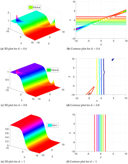
Figure 1. Dynamics of solution of Example 1 for a few fractional orders. The values of the parameters are taken as: $\alpha =1$, $\beta =1$, $\gamma =-0.05$, and $\delta =0.001$.

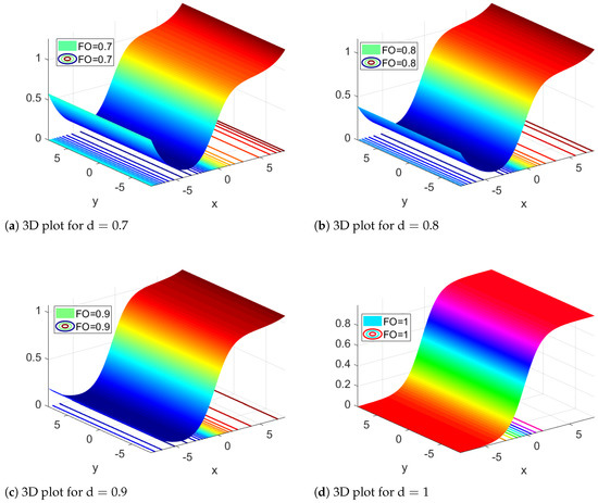
Figure 2. Dynamics of solution of Example 2 for a few fractional orders. The values of the parameters are taken as: $\alpha =1$, $\beta =1$, $\gamma =-0.05$, and $\delta =0.001$.

Table 1. Error analysis between solutions obtained using the proposed method for $\mathrm{d}=1$, $t=0.02$ for Example 1 and i $=\sqrt{-1}$.

(x, y, t)	Exact	Approximate	∣Exact-Approximate∣
(−10, −10, 0.05)	−1.0000 + 0.0000i	−0.9999 + 0.0000i	0.0001
(−8, −8, 0.05)	−1.0000 + 0.0000i	−0.9996 + 0.0001i	0.0005
(−6, −6, 0.05)	−1.0000 + 0.0000i	−0.9967 + 0.0009i	0.0034
(−4, −4, 0.05)	−1.0000 + 0.0000i	−0.9760 + 0.0062i	0.0247
(−2, −2, 0.05)	−0.9967 + 0.0009i	−0.8454 + 0.0343i	0.1550
(0, 0, 0.05)	−0.5182 + 0.0648i	−0.4458 + 0.0657i	0.0724
(2, 2, 0.05)	−0.0038 + 0.0010i	−0.0870 + 0.0208i	0.0855
(4, 4, 0.05)	−0.0000 + 0.0000i	−0.0126 + 0.0033i	0.0130
(6, 6, 0.05)	−0.0000 + 0.0000i	−0.0017 + 0.0005i	0.0018
(8, 8, 0.05)	−0.0000 + 0.0000i	−0.0002 + 0.0001i	0.0002
(10, 10, 0.05)	−0.0000 + 0.0000i	−0.0000 + 0.0000i	0.0000

Table 2. Error analysis between solutions obtained using the proposed method for $\mathrm{d}=1$, $t=0.02$ for Example 2 and i $=\sqrt{-1}$.

(x, y, t)	Exact	Approximate	∣Exact-Approximate∣
(−10, −10, 0.05)	−0.0004 − 0.0001i	−0.0101 + 0.0167i	0.0194
(−8, −8, 0.05)	−0.0033 − 0.0009i	−0.0070 + 0.0053i	0.0072
(−6, −6, 0.05)	−0.0240 − 0.0062i	−0.0256 − 0.0039i	0.0028
(−4, −4, 0.05)	−0.1548 − 0.0342i	−0.1561 − 0.0335i	0.0015
(−2, −2, 0.05)	−0.5820 − 0.0632i	−0.5835 − 0.0629i	0.0016
(0, 0, 0.05)	−0.9132 − 0.0208i	−0.9144 − 0.0203i	0.0013
(2, 2, 0.05)	−0.9874 − 0.0033i	−0.9887 − 0.0018i	0.0020
(4, 4, 0.05)	−0.9983 − 0.0005i	−1.0011 + 0.0037i	0.0050
(6, 6, 0.05)	−0.9998 − 0.0001i	−1.0070 + 0.0114i	0.0135

7. Conclusions

In this paper, we have discussed the extended version of the KdV equation under the fractional operator. We have considered the fractional operator with the convolution of non-singular and non-local kernels. We derived qualitative properties regarding the existence, uniqueness, and stability of the solution. We have used the Laplace transform with a decomposition method to derive the solution of the considered KdV-mKdV equation. We have proved the convergence of the proposed method. Furthermore, the Picard stability of the solution of the considered equation has been proved using fixed-point theory. We have visualized all the obtained solutions via 3D and contour plots. We have observed the hidden wave dynamics for the fractional order from the simulations, which can not be seen via the integer order. We have considered two examples whose solutions exhibit kink behaviour. The effects of the fractional order on the shape of kink behaviour are shown in Figure 1 and Figure 2. We concluded that the fractional operator has a significant effect on the shape of the kink solution of the proposed KdV-mKdV equation.

In the literature, several researchers have pointed out issues relating to fractional operators. For instance, Cresson et al. [27] described issues including Leibniz and chain rule properties for various extensions of Riemann–-Liouville fractional derivatives. The issue of the Leibniz rule in fractional operators was discussed by Tarasov in his short paper [28]. He pointed out that the Leibniz rule is only valid for integer-order operators, but not for fractional operators. Ortigueira highlighted another issue in the fractional calculus literature. He proved that the Riemann–Liouville fractional derivative of a constant is not zero (for more details see [29]). Several approaches can be applied to further investigate the considered equation in future. Some well-known operators, such as fractal-fractional operators, stochastic operators and fuzzy operators can be used to further investigate the considered equation in future projects.

References

- Wazwaz, A.M. Partial Differential Equations and Solitary Waves Theory; Springer: Berlin/Heidelberg, Germany, 2010. [Google Scholar]
- Salas, A.; Kumar, S.; Yildirim, A.; Biswas, A. Cnoidal waves, solitary waves and painlevé analysis of the 5th order KdV equation with dual-power law nonlinearity. Proc. Rom. Acad. A 2013, 14, 28–34. [Google Scholar]
- Ji, J.L.; Zhu, Z.N. On a nonlocal modified Korteweg-de Vries equation: Integrability, Darboux transformation and soliton solutions. Commun. Nonlinear Sci. Numer. Simul. 2017, 42, 699–708. [Google Scholar] [CrossRef]
- Gurses, M.; Pekcan, A. Nonlocal modified KdV equations and their soliton solutions by Hirota method. Commun. Nonlinear Sci. Numer. Simul. 2019, 67, 427–448. [Google Scholar] [CrossRef]
- Alquran, M. Optical bidirectional wave-solutions to new two-mode extension of the coupled KdV–Schrodinger equations. Opt. Quantum Electron. 2021, 53, 588. [Google Scholar] [CrossRef]
- Malik, S.; Kumar, S.; Das, A. A (2+1)-dimensional combined KdV–mKdV equation: Integrability, stability analysis and soliton solutions. Nonlinear Dyn. 2022, 107, 2689–2701. [Google Scholar] [CrossRef]
- Alqahtani, R.T.; Ahmad, S.; Akgül, A. Dynamical analysis of bio-ethanol production model under generalized nonlocal operator in Caputo sense. Mathematics 2021, 9, 2370. [Google Scholar] [CrossRef]
- Khan, Z.A.; Khan, J.; Saifullah, S.; Ali, A. Dynamics of hidden attractors in four-dimensional dynamical systems with power law. J. Funct. Spaces 2022, 2022, 3675076. [Google Scholar] [CrossRef]
- Saifullah, S.; Ali, A.; Irfan, M.; Shah, K. Time-fractional Klein–Gordon equation with solitary/shock waves solutions. Math. Probl. Eng. 2021, 2021, 6858592. [Google Scholar] [CrossRef]
- Baleanu, D.; Jajarmi, A.; Mohammadi, H.; Rezapour, S. A new study on the mathematical modelling of human liver with Caputo–Fabrizio fractional derivative. Chaos Solitons Fractals 2020, 134, 109705. [Google Scholar] [CrossRef]
- Baleanu, D.; Jajarmi, A.; Hajipour, M. A new formulation of the fractional optimal control problems involving Mittag–Leffler nonsingular kernel. J. Optim. Theory Appl. 2017, 175, 718–737. [Google Scholar] [CrossRef]
- Gulalai; Rihan, F.A.; Ahmad, S.; Ullah, A.; Al-Mdallal, Q.M.; Akgül, A. Nonlinear analysis of a nonlinear modified KdV equation under Atangana Baleanu Caputo derivative. AIMS Math. 2022, 7, 7847–7865. [Google Scholar] [CrossRef]
- Liua, X.; Arfan, M.; ur Rahman, M.; Fatima, B. Analysis of SIQR type mathematical model under Atangana-Baleanu fractional differential operator. Comput. Methods Biomech. Biomed. Eng. 2022, 1–15. [Google Scholar] [CrossRef] [PubMed]
- Sadiq, G.; Ali, A.; Ahmad, S.; Nonlaopon, K.; Akgül, A. Bright Soliton Behaviours of Fractal Fractional Nonlinear Good Boussinesq Equation with Nonsingular Kernels. Symmetry 2022, 14, 2113. [Google Scholar] [CrossRef]
- Shah, N.A.; Alyousef, H.A.; El-Tantawy, S.A.; Shah, R.; Chung, J.D. Analytical Investigation of Fractional-Order Korteweg–De-Vries-Type Equations under Atangana–Baleanu–Caputo Operator: Modeling Nonlinear Waves in a Plasma and Fluid. Symmetry 2022, 14, 739. [Google Scholar] [CrossRef]
- Ahmad, H.; Tariq, M.; Sahoo, S.K.; Askar, S.; Abouelregal, A.E.; Khedher, K.M. Refinements of Ostrowski Type Integral Inequalities Involving Atangana–Baleanu Fractional Integral Operator. Symmetry 2021, 13, 2059. [Google Scholar] [CrossRef]
- Cao, Q.H.; Dai, C.Q. Symmetric and Anti-Symmetric Solitons of the Fractional Second- and Third-Order Nonlinear Schrödinger Equation. Chin. Phys. Lett. 2021, 38, 090501. [Google Scholar] [CrossRef]
- Li, P.; Li, R.; Dai, C. Existence, symmetry breaking bifurcation and stability of two-dimensional optical solitons supported by fractional diffraction. Opt. Express 2021, 29, 3193–3210. [Google Scholar] [CrossRef]
- Mou, D.S.; Dai, C.Q. Vector solutions of the coupled discrete conformable fractional nonlinear Schrödinger equations. Optik 2022, 258, 168859. [Google Scholar] [CrossRef]
- Chen, Y.X. Combined optical soliton solutions of a (1+1)-dimensional time fractional resonant cubic-quintic nonlinear Schrödinger equation in weakly nonlocal nonlinear media. Optik 2020, 203, 163898. [Google Scholar] [CrossRef]
- Fang, J.J.; Mou, D.S.; Zhang, H.C.; Wang, Y.Y. Discrete fractional soliton dynamics of the fractional Ablowitz-Ladik model. Optik 2021, 228, 166186. [Google Scholar] [CrossRef]
- Bo, W.B.; Liu, W.; Wang, Y.Y. Symmetric and antisymmetric solitons in the fractional nonlinear schrödinger equation with saturable nonlinearity and PT-symmetric potential: Stability and dynamics. Optik 2022, 255, 168697. [Google Scholar] [CrossRef]
- Ullah, I.; Ali, A.; Saifullah, S. Analysis of time-fractional non-linear Kawahara Equations with power law kernel, Chaos, Solitons. Fractals X 2022, 9, 100084. [Google Scholar]
- Saifullah, S.; Ali, A.; Khan, Z.A. Analysis of nonlinear time-fractional Klein-Gordon equation with power law kernel. AIMS Math. 2021, 7, 5275–5290. [Google Scholar] [CrossRef]
- Khan, A.; Akram, T.; Khan, A.; Ahmad, S.; Nonlaopon, K. Investigation of time fractional nonlinear KdV-Burgers equation under fractional operators with nonsingular kernels. AIMS Math. 2023, 8, 1251–1268. [Google Scholar]
- Atangana, A.; Baleanu, D. New fractional derivatives with nonlocal and non-singular kernel: Theory and application to heat transfer model. Therm. Sci. 2016, 20, 763–769. [Google Scholar] [CrossRef]
- Cresson, J.; Szafrańska, A. Comments on various extensions of the Riemann–Liouville fractional derivatives: About the Leibniz and chain rule properties. Commun. Nonlinear Sci. Numer. Simul. 2020, 82, 104903. [Google Scholar] [CrossRef]
- Tarasov, V.E. No violation of the Leibniz rule. Fract. Deriv. 2013, 18, 2945–2948. [Google Scholar]
- Ortigueiram, M.D. Comments on “Modeling fractional stochastic systems as non-random fractional dynamics driven Brownian motions”. Appl. Math. Model. 2009, 33, 2534–2537. [Google Scholar]
Publisher’s Note: MDPI stays neutral with regard to jurisdictional claims in published maps and institutional affiliations. |
© 2022 by the authors. Licensee MDPI, Basel, Switzerland. This article is an open access article distributed under the terms and conditions of the Creative Commons Attribution (CC BY) license (https://creativecommons.org/licenses/by/4.0/).