One-Parameter Statistical Methods to Recognize DDoS Attacks

Abstract

Within our academic high-speed network infrastructure which is used for connecting all universities and high schools in our country to the Internet, there are thousands of cybersecurity attacks occurring every day. That is why, within our SANET II project, an effort has been made to create a self-learning system without a teacher, which would be able to quickly adapt to arbitrary traffic and recognize DDoS attacks on time, even in high-speed networks, with a potential simple implementation into a hardware probe. In the article, we deal with the Hurst and autoregression coefficients and the coefficient of variation. We test the coefficients on simulated data and on real records of attacks. For early machine recognition of the attack, we propose the so-called predicting $\sigma$-tunnel. The obtained results can lead to the investigation of other prediction methods that would improve the early recognition of an attack.

1. Introduction

In today’s digital age, technology has a remarkable impact on our day-to-day lives, and it helps to simplify many tasks. However, this also means that if one of those tools gets attacked by malicious actors or is misused in any other way, it becomes a huge cybercrime issue. Luckily, cybersecurity is becoming very important in countries worldwide, which means that more and more security operation centers (SOCs) are established and help to raise awareness of cybersecurity’s importance. Our university is connected to the Internet using the Slovak Academic Network (SANET) which is the network provider interconnecting all universities and high schools across Slovakia. This nationwide network is also facing a huge number of daily cybersecurity threats ranging from simple brute-force login attacks to distributed denial-of-service (DDoS) attacks, which are becoming more frequent and effective every year.

The end goal of DDoS attacks is the same as that of DoS attacks, where the attacker is trying to render the service provided by a remote server inaccessible to users or to slow down the responses of the server. However, DDoS attacks are distributed because they come from a large number of sources called bots, which are usually part of a botnet controlled by a command-and-control server operated by the attacker. There are many reasons for this type of attack, usually to dispose of competition or to demonstrate against some policies or laws.

DDoS attacks are, according to [1], categorized into three groups. The first group is represented by volume-based attacks, causing network congestion and exhausting network bandwidth between users and the target service or the rest of the Internet. The second group are protocol attacks exploiting vulnerabilities in a network protocol. This can happen when an attacker creates a large number of TCP connections, attempting to exhaust the limit of possible TCP connections that are configured in network devices, such as firewalls, servers or even load balancers. The third and the most dangerous type is an application attack. This type of attack is trying to misuse some property of an application or service. It is usually very effective, so there is no need for a large number of attacking devices, or high-bandwidth traffic. That is why it is hard to detect and mitigate those attacks.

Today’s attacks are highly sophisticated since they use any of the three categories in combination. DDoS attacks are most of the time also used as a disguise for more advanced threats such as malware. Using this technique, it is harder for network security teams to spot an injection of such an advanced threat, which can further be used to obtain critical information from inside of infected devices. Those infected devices can further become a part of the botnet, which is a remotely controlled group of devices, also called “zombie computers” [2], usually consisting of millions of devices. As the device was infected covertly, it can be part of a botnet even without the owner’s knowledge. As the number of botnet devices is high, they can generate a staggering amount of traffic, easily exceeding the DDoS attack’s target bandwidth. Cybercriminals also sell or lease already-created botnets, as it is time-consuming and a large amount of knowledge is needed to create new ones.

Defense against DDoS attacks consists of three main parts: monitoring, detection and response [3]. Monitoring is a crucial part as it collects information about the network services provided to users. Detection methods are running on top of data gathered through monitoring to identify patterns and anomalies or incidents inside the network. The response part works after the detection methods detect an attack. The firewall rules are added as the first line of defense and the threat is recorded and reported to the network security team.

Statistical methods, such as entropy, correlation and covariance are considered to be the most common methods of detecting DDoS attacks and analyzing and identifying anomalies in network flow. The whole traffic capture or only individual network packets can be transformed to network characteristic parameters further used as inputs into statistical methods. Statistical or correlation measures are useful for analyzing network traffic. They can also distinguish attacks in network flows [4]. These methods can be referred to as machine learning methods with a teacher.

Our research is unique as we are searching for the characteristics of the network flow that would be able to respond in time to a major change in the nature of the traffic flow containing a DDoS attack. The considered characteristics are first calibrated on normal nonattacking network traffic to standard values and after the calibration is done the method is able to recognize the upcoming attack. That is why we use one-parameter methods of machine learning without a teacher for the research presented in this paper.

In the first part of Section 3, we deal with the methodology for IP flows description. The next part explains the motivation for the research presented in this article. The last part of that section describes the statistical methods used to detect attacks: Hurst coefficient, autoregressive coefficient and coefficient of Variability. Section 4 deals with simulations of IP flows using the Markov two-state on–off model. Section 5 describes the DDoS attacks detection on five selected real datasets of captured traffic. In Section 6, we propose our own symmetrical prediction tunnel designed for attack recognition using machine learning without a teacher. We summarize the results, observations and suggestions for further research direction in Section 7.

2. Related Work

There are several mathematical principles and models which try to identify a flood attack. The basic features include tracking changes in the statistical moments of network flows, such as the mean intensity, variance, spiciness coefficient and tracking changes in the probability distribution of packet occurrence, e.g., [5]. The work in [6] used four measures of periodicity, the kurtosis, skewness and self-similarity of a time series to compare histograms of the number of packets during normal and attack traffic. The authors in [7] used the fitting of the probability distribution of the monitored IP traffic with continuous distributions using three statistical moments and then tested the hypotheses about the occurrence of a DDoS attack. Using the change of autocorrelation at the onset of a DDoS attack was studies by, e.g., [8]. The autocorrelation in the convolution of legitimate and attack traffic (cross-correlation method) was addressed by [9]. Estimating the strength of a DDoS attack using a multiple regression analysis is discussed in detail in [10]. The use of a regression model for predicting the number of zombies in DDoS attacks can be find in [11].

An important statistical characteristic that describes the self-similarity of a time series is the Hurst coefficient or parameter. The Hurst parameter was used to identify a DDoS attack in [12]. The authors in [13] compared the average Hurst values of normal and offensive traffic. The suitability of using the Hurst coefficient is also discussed in [14].

A combination of several methods, for example the correlation and Hurst parameter, can be found in [15]. The authors of [16] used an autoregressive system for estimating the variance of the Hurst coefficient for the purpose of detecting changes in the flow. The research in [17] used self-similarity and Renyi entropy. The application of fractal analysis to detect attacks can be found in [18]. The authors in [19] dealt with a combination of fractal and recurrent functions. Different machine learning (ML) algorithms were used by [20]. The authors used GAN networks in [21], and the authors of the paper [22] dealt with anomaly detection using autoencoders and deep convolutional GAN networks. In [23], a GAN network with two discriminators was also used for detection.

A popular and effective method is the PCA decomposition method. The authors of the article [24] used a PCA as an indicator of anomalies in IP flow. A dimensionality reduction of the dataset of IP flow attributes using a PCA and the subsequent detection using entropy was used in [25].

In [26], the authors looked for an optimal solution between several metrics and entropies for detection. The authors in [27], to recognize relatively new low-rate DDoS attacks, used the entropy between exceptions in packet size between normal and attacking traffic. Queue management algorithms (RED and REM) were used against DDOS attacks in [28].

Other methods include detecting attacks using wavelets (wavelet analysis) [29,30,31], using blockchain [32], genetic algorithms and random forest [33] and the use of various spectral and cluster analyses that have been successful in image and sound recognition as well.

The authors of the paper [34] described the occurrence of DDoS attacks in IoT networks and proposed a method for the mitigation of these attacks. In this paper, we try to describe a design of a sufficiently robust system that can also be used in IoT networks for the purpose of detecting DDoS attacks.

In contrast to the majority of the mentioned works, we aim to find computationally undemanding statistical variables that would derive their values from the number of packets of the input flow in a given calculation window and would react in time to the start of a flood attack with a significant change for the timely detection of a DDoS attack. Next, we want to develop prediction methods (without a teacher) for the reliable machine recognition of a significant change in the values of the monitoring variables.

3. Methods

The set of values of the monitored parameters, on which the given method determines that the analyzed network flow represents legitimate traffic, is called the acceptable area. The set of values on which the attack is identified is called the critical area. Most of the mathematical methods used to detect DDoS attacks use standard datasets, e.g., MIT outside normal traffic, CAIDA-2007 DDoS attack traffic, TUDDoS dataset, etc. These datasets are used to create acceptable and critical areas using machine learning, or to directly compare parameter values obtained from observed network traffic with values calculated in a given dataset. Our overall intention was to determine a set of mathematical methods that would recognize potential DDoS attacks while the network is running without prior learning on test datasets. Assuming the application of the method at a time when the monitored network IP flow is in a state of legitimate operation, our method itself calculates the values of the acceptable area for the given flow. When monitoring IP traffic, we used mutually overlapping time windows, while a new window was created by loading the next sample from the monitored IP traffic.

We focused on static parameters that we assume would successfully detect the change in IP network flow structure in consecutive time windows. We selected the Hurst coefficient, the autoregressive coefficient and the coefficient of variability.

3.1. IP Flow Description

A packet flow generated by a network device is one of the basic IP network elements. There are several concepts for describing packet flow. For example, in a deterministic IP network model, network calculus and subadditive curves are used to describe flows [35]. One of the stochastic descriptions of network flows is to use the effective bandwidth of the observed flow [36,37].

A basic method of description of network flow is to use process $A(r,s)$ (arrival process), which represents the number of packets in the interval $\langle r,s\rangle$. Another method is the usage of the variables $T_i$, which describe the time-gap duration between the occurrence of individual packets, as shown in Figure 1.

In general, we assume that the flow representing IP traffic is random, with $A(r,s)$ representing a stochastic process and $T_i$ corresponding random variables. Another simplification is that we take into account only the so-called stationary random processes. Simply put, all probabilistic characteristics of a stationary process are invariant with respect to time. It does not matter in which time interval we started to observe the flow, it only depends on the length of the observation, as shown in Figure 2.

For a stationary process, in which it does not matter where in time the observed time window is located as it only depends on the length of the observed window, we can introduce a simplified designation $A\left(t\right)$:

$$\forall a\in R^{+};A(a,a+t)=A(0,t)=A\left(t\right)$$

(1)

The stationary process does not change its probability characteristics over time. Therefore, the random variables $T_i$, which describe the i gaps in the packet flow, have the same probability distribution. We can use the same random variable T for all gaps, which has the distribution function $F\left(t\right)$, $T\sim F\left(t\right)$.

If the IP traffic is measured in given time slots, the process $A\left(t\right)$ consists of the so-called increments $a\left(i\right)$ that record the occurrence of packets in time slots i. No packet occurs at time zero, therefore $A\left(0\right)=a\left(0\right)=0$:

$$A\left(t\right)=\sum _{i=1}^{t}a\left(i\right),a\left(t\right)=A\left(t\right)-A(t-1),$$

(2)

If we consider a time window of length n time slots, the basic characteristics of an IP flow, the average rate ${\lambda }_{avg}$ and peak rate ${\lambda }_{peak}$, have the shape:

$${\lambda }_{avg}=EA\left(n\right),{\lambda }_{peak}=\underset{1\le i\le n}{max}a\left(i\right)=n$$

(3)

Whenever it is more convenient, we use notation $a_i$ instead of $a\left(i\right)$ for the increments of the IP network flow.

3.2. Motivation

Our university is connected to the Internet via the academic high-speed network infrastructure called Slovak academic network (SANET). Devices connected to this network are constantly under cybersecurity attacks from threat actors with varied skills, ranging from simple brute-force SSH or RDP attacks to more severe DDoS attacks. Protecting this network because of its high speed is costly as more and more powerful network devices are needed to mitigate more sophisticated attacks. That is why effort has been made to find computationally relatively simple statistical methods and create a self-learning system without a teacher that would detect the occurrence of a DDoS attack in real traffic. Subsequently, these methods are supposed to be implemented in a hardware probe for the purpose of monitoring IP traffic in real time. We deal with this issue within the SANET II project—“Research in the SANET network and possibilities for its further use and development”.

The overall goal of the SANET II project is to apply research results in the form of innovative distribution network services and technologies with an emphasis on security and reliability. The methods and principles proposed by the project will enable a faster onset of technologies for more efficient and safer transmission of specific data. The goal is to create new models and methods of distribution with regard to future interdisciplinary adaptation. Innovation in this area of network infrastructure development will not only help the scientific and research community to better distribute, store and share R&D data, but will also open up the possibilities of adaptation in the field of Industry 4.0, in the form of a modification of the proposed concepts for machine communication mechanisms in a large-scale network environment. Out team is working on this research in the field of advanced monitoring of flows and in the evaluation of security events for networks and cloud computing systems. Several articles were published by our team on the topic of CC systems [38], their security architecture [39], the management of cybersecurity incidents and on creating a packet capture infrastructure for creating valuable datasets [40].

In a standard DDoS attack, there is an increase peak rate and average rate of flow increments. However, monitoring only these rates is not enough. The peak rate can randomly acquire a high value even during standard operation. The average rate value, which is calculated in a selected time window, increases relatively slowly when a DDoS attack starts. We present the claim in the following Figure 3:

Figure 3 shows a simulation for a Bernoulli flow of bits with a length of 1600 time slots (ts). In the first three quarters of the flow, the increments have a binomial distribution $a\left(i\right)\sim Bi(1,0.5)$ and the mean of the increments is $Ea\left(i\right)=0.5\mathrm{bit}/\mathrm{ts}$. In the last quarter, the increments have distribution $a\left(i\right)\sim Bi(1,0.9)$ and the mean of the increments is $Ea\left(i\right)=0.9\mathrm{bit}/\mathrm{ts}$. For this flow, we gradually calculated the values of the average rate and Hurst coefficient. We deal with this in more detail in the next section. We first estimated the parameter values from increments in a time window of 512 ts, then we moved the time window by one time slot and recalculated the parameter values. In the picture, we can see that when loading, for example, 10% attack traffic (ts = 1251), the value of the average rate changed from 0.5 to almost 0.6, while the value of the Hurst coefficient changed significantly from 0.4 to 0.9. We can see that the Hurst parameter reacted significantly faster to a DDoS attack than the average rate of the flow.

System process flow: Using the online live traffic flow, the self-learning adaptive system calibrates the admissible values of the statistical parameters, describing the normal operation (it learns what the traffic looks like). From these values, it creates a prediction tunnel with which it can detect a DDoS in time. An example of the network topology where the probe is a self-learning system method is shown in Figure 4:

3.3. One-Parameter Statistical Methods

We assumed that with a standard DDoS attack, not only the average rate of the flow increased, but as a result of the generation of a large number of flood packets, the variance of the flow decreased, or the entire probabilistic structure of the flow changed. Therefore, we tried to find methods that recognized the structure of the flow in a relatively simple way. Among the one-parameter statistical methods, we chose the Hurst coefficient, autoregression coefficient and coefficient of variance.

3.3.1. Hurst Coefficient

The Hurst exponent is used as a measure of long-term memory in time series. This refers to the autocorrelation of the series and the rate at which the autocorrelation decreases with increasing time distance between pairs of time series values.

The Hurst exponent quantifies the relative tendency of the time series either to strongly decrease towards the average, or cluster in a certain direction. The value $H\in 〈0.5,1〉$ indicates a time series with a long-term positive autocorrelation, a value in the range $H\in 〈0,0.5〉$ indicates a time series with a long-term switching between high and low values. The value H = 0.5 may indicate a completely uncorrelated series, for example a Poisson process, or a time series in which the absolute values of the autocorrelation decrease exponentially fast to zero.

The Hurst coefficient is used in several areas of applied mathematics, including fractals and chaos theory, long-term memory processes, spectral analysis and in sizing network parameters in queueing theory [41].

The Hurst coefficient cannot be determined analytically, it can only be estimated statistically. There are several methods used to estimate the exponent but we list the most frequently used method, the R/S analysis [42].

We have a time series $X_1,X_2,\dots ,X_n$ from which we select a sample of data. We calculate the accumulated relative deviations from the average value:

$$Y_{t,n}=\sum _{i=1}^t|X_i-\overline{X}|,t=1,\dots ,n$$

(4)

We calculate the range determined as the difference between the maximum and minimum accumulated deviation for a given period and also the standard deviation:

$$R_n=\underset{i\le t\le n}{max}{Y}_{t,n}-\underset{i\le t\le n}{min}{Y}_{t,n},S_n=\sqrt{{\displaystyle \frac{1}{n-1}}\sum _{i=1}^n|X_i-\overline{X}|}$$

(5)

We normalize the range $R_n$ by the standard deviation $S_n$, which gives the scaling range

$${\left(R/S\right)}_n=R_n/S_n$$

(6)

The values of the division of statistical deviations ${(R/S)}_n$ grow exponentially with increasing n according to the following equation:

$${\left(R/S\right)}_n\approx C·n^H$$

(7)

where C is a constant and H is the Hurst exponent. There are several methods for estimating the value of the Hurst coefficient. One possibility is to calculate the slope of the regression line, which represents the graph of $ln{(R/S)}_n$ vs. $ln\left(n\right)$. This relationship can be expressed analytically by the equation:

$$ln{\left(R/S\right)}_n=lnC+H·lnn$$

(8)

To estimate the Hurst parameter, the ${(R/S)}_n$ values of the statistic approximates a regression line. The Hurst parameter represents the tangent of this line.

3.3.2. Autoregression Coefficient AR(1)

An autoregressive model (AR) is a linear model used in the analysis and prediction of time series. Any observation in the time series depends only on the value of the previous observation and on the random component.

The autoregressive model $AR\left(n\right)$ assumes that the considered random process ${\left\{X_t\right\}}_{t\in T}$ has the structure

$$X_t={\beta }_1{X}_{t-1}+{\beta }_2{X}_{t-2}+\cdots +{\beta }_n{X}_{t-n}+{\epsilon }_t,$$

(9)

while random variables ${\epsilon }_t$ represent model errors; we assume that they are uncorrelated with each other and have a normal probability distribution ${\epsilon }_t\sim N(0,{\sigma }^2)$ (random variables ${\epsilon }_t$ constitute white noise) [43].

Let the values $(a_1,a_2,\dots ,a_N)$ (increments of flow) represent N realizations of the random process ${\left\{X_t\right\}}_{t\in T}$. If the $AR\left(n\right)$ model is valid, the realizations form the following structure

$$a_t={\beta }_1{a}_{t-1}+{\beta }_2{a}_{t-2}+\cdots +{\beta }_n{a}_{t-n}+{ϵ}_t,$$

(10)

for $t=n+1,\dots ,N$. For all N measurements, we get a matrix notation

$$\left[\begin{array}{c}{a}_{n+1}\\ ⋮\\ a_N\end{array}\right]=\left(\begin{array}{ccc}{a}_n& \dots & a_1\\ ⋮& \ddots & ⋮\\ a_{N-1}& \dots & a_{N-n}\end{array}\right)\left[\begin{array}{c}{\beta }_1\\ ⋮\\ {\beta }_n\end{array}\right]+\left[\begin{array}{c}{ϵ}_{n+1}\\ ⋮\\ {ϵ}_N\end{array}\right].$$

(11)

If we denote the matrix of all N values of the dependent variable $a_t$ as $\mathbf{y}$ and $\mathsf{ϵ}$ as the vector of measured errors, we can describe the autoregressive model using the standard multivariate linear regression model

$$\mathbf{y}=\mathbf{X}\mathsf{\beta }+\mathsf{ϵ}.$$

(12)

Estimates of unknown parameters $\mathsf{\beta }={({\beta }_1,\dots ,{\beta }_n)}^T$ are obtained by the least squares method (LSM), minimizing the sum of squared errors (residues)

$$min\mathsf{ϵ}{\mathsf{ϵ}}^T=min\sum _{i=n+1}^N{ϵ}_i^2.$$

(13)

According to [44,45] the sum of residuals $\mathsf{ϵ}{\mathsf{ϵ}}^T$ acquires a minimum for the vector $\hat{\mathsf{\beta }}$ which is a solution of the equation

$${\mathbf{X}}^{\mathbf{T}}\mathbf{X}\mathsf{\beta }={\mathbf{X}}^{\mathbf{T}}\mathbf{y}.$$

(14)

If the matrix $\mathbf{X}$ has full rank, $N-n-1\ge n$, then the solution (14) has the form

$$\hat{\mathsf{\beta }}={\left({\mathbf{X}}^{\mathbf{T}}\mathbf{X}\right)}^{-1}{\mathbf{X}}^{\mathbf{T}}\mathbf{y},$$

(15)

while the solution $\hat{\mathsf{\beta }}$ is at the same time an unbiased and consistent estimate of the parameters $\mathsf{\beta }$, which means $E\left(\hat{\mathsf{\beta }}\right)=\mathsf{\beta }$ and $\underset{N\to \infty }{lim}D\left(\hat{\mathsf{\beta }}\right)=0$.

In the case where $n=1$, we assume that the random variable $X_t$ depends linearly on the previous random variable $X_{t-1}$

$$X_t=c{X}_{t-1}+{\epsilon }_t,$$

(16)

whereby we denote the parameter c as the autoregression coefficient. We denote such a process as AR(1).

For increments of flow $(a_1,a_2,\dots ,a_N)$ in a given time window of length N, the system of Equation (11) has the form:

$$\left[\begin{array}{c}{a}_{n+1}\\ ⋮\\ a_N\end{array}\right]=\left[\begin{array}{c}{a}_n\\ ⋮\\ a_{N-1}\end{array}\right]c+\left[\begin{array}{c}{ϵ}_{n+1}\\ ⋮\\ {ϵ}_N\end{array}\right].$$

(17)

The estimate of the autoregressive coefficient c is obtained from the formula:

$$\hat{c}={\left({\mathbf{X}}^{\mathbf{T}}\mathbf{X}\right)}^{-1}{\mathbf{X}}^{\mathbf{T}}\mathbf{y}={\left(\sum _{i=n}^{N-1}{a}_i^2\right)}^{-1}·\sum _{i=n}^{N-1}{a}_i{a}_{i+1}$$

(18)

3.3.3. Coefficient of Variation

The coefficient of variation of the random variable X represents the ratio between the standard deviation and the mean value of X

$$\nu ={\displaystyle \frac{{\sigma }_T}{E\left[T\right]}}$$

(19)

We obtain an estimate of the coefficient of variation for the currently examined time window $(a_1,a_2,\dots ,a_N)$ from the ratio between the sample standard deviation and the average speed:

$$\hat{\nu }={\displaystyle \frac{s}{{\lambda }_{avg}}}\mathrm{where}s=\sqrt{{\displaystyle \frac{1}{N-1}}\sum _{i=n}^{N-1}{\left(a_i-{\lambda }_{avg}\right)}^2}\mathrm{and}{\lambda }_{avg}=\frac{1}{N}\sum _{i=n}^{N-1}{a}_i$$

(20)

The coefficient of variation expresses the degree of variability of the observed random event [46]. In the case of a standard DDoS attack, we expect a significant increase in the average rate ${\lambda }_{avg}$ of the number of packets in a given time window, but at the same time a decrease in the dispersion of the network flow of packets generated by the attacker. Under these assumptions, the coefficient of variation could serve as a significant identifier of a DDoS attack.

We first verified the effectiveness of the individual coefficients in DDoS attack detection on simulated IP flows using several different scenarios.

4. Simulations

We verified the effectiveness of the individual coefficients in DDoS attack detection in the first approach on simulated IP flows using two different scenarios.

Scenario 1: In the first scenario, we simulated a standard DDoS attack. The simulated flow consisted of three parts of equal length. The first part simulated normal network traffic, the second part a DDoS attack with at least twice the average rate, and the third part was again legitimate network traffic. In addition to the change in intensity, we also tested cases with a reduced variance or with an overall different character of the flow.

Scenario 2: The second scenario simulated recurring DDoS attacks, when a rapid burst of packets is repeated after a certain period of time. The total simulated flow consisted of periods when 90% was legitimate network traffic and 10% was attacking network traffic. It was actually a simulation in the context of the current so-called low-rate DDoS attacks, which are carried out cyclically in short bursts of packets.

We calculated the individual values of the selected parameters in the time window $\Delta t$ of the given length. Next, we shifted the time window by one time slot and repeated the calculation of values. At the start of the DDoS attack, the first time window contained 99% of normal traffic and 1% of attack traffic. With this method of calculating parameter values, we could observe at what volume of recorded attack traffic our selected parameters reacted significantly.

Scenario 1

To simulate different scenarios, we chose a two-state Markov modulated regular process (MMRP) [47]. This Markov process chain with discrete time consists of two states between which it randomly switches in each time slot. The probabilities of switching between states are denoted as $\alpha$ and $\beta$. In the first state, the process generates data deterministically (regular flow of one sequences), in the second state it generates zeros. We also refer to such a process as an on/off source of IP traffic. The probability distribution of the states of the chain, which stabilizes over time, is denoted as $\mathsf{ß}=({\pi }_1,{\pi }_2)$ and we call it the stationary distribution. An analysis of the MMRP can be found in [48]. Transition graph of Markov chain has form as shown in Figure 5.

We calculated the stationary distribution:

$$\mathsf{\pi }=\mathsf{\pi }\mathbf{P}\Rightarrow {\left[\mathbf{E}-\mathbf{P}\right]}^T{\mathsf{\pi }}^T={\mathbf{0}}^T$$

$$\mathbf{P}=\left[\begin{array}{cc}1-\alpha & \alpha \\ \beta & 1-\beta \end{array}\right],{\left[\mathbf{E}-\mathbf{P}\right]}^T=\left[\begin{array}{cc}\alpha & -\beta \\ -\alpha & \beta \end{array}\right]$$

$$\Rightarrow \alpha {\pi }_1-\beta {\pi }_2=0\Rightarrow {\pi }_2={\displaystyle \frac{\alpha }{\beta }}{\pi }_1\Rightarrow$$

$${\pi }_1+{\displaystyle \frac{\alpha }{\beta }}{\pi }_1=1\Rightarrow {\pi }_1\left[1+{\displaystyle \frac{\alpha }{\beta }}\right]=1$$

$${\pi }_1={\displaystyle \frac{\beta }{\alpha +\beta }},{\pi }_2={\displaystyle \frac{\alpha }{\alpha +\beta }},Ea\left(i\right)={\pi }_1={\displaystyle \frac{\beta }{\alpha +\beta }}$$

The probability characteristics of the MMRP depend on the parameters $\alpha$ and $\beta$. Thanks to that, we could use MMRP to simulate various types of flows. If $\alpha +\beta =1$, we obtain a Bernoulli flow; if $\alpha ,\beta \to 0$, we have an on–off bursty flow; if $\alpha ,\beta \to 1$, we get a regular or deterministic process.

For a good visualization of the experiments, we chose 32-bit flows, which we obtained by summing the flood 0/1 sequences generated by the MMRP process.

In Scenario 1.1, we simulated the first third of the record, which represented standard network operation, using a Bernoulli process with increments $a\sim Bi(32,0.5)$ with $Ea\left(i\right)=16\mathrm{bit}/\mathrm{ts}$. The Bernoulli process is suitable as a flow model for the core network or in the case of aggregating a large number of independent flows. The second third represented a DDoS attack, which we simulated as a Bernoulli process with increments $a\sim Bi(32,0.9)$. The mean rate of flow thus increased to $Ea\left(i\right)=28.8\mathrm{bit}/\mathrm{ts}$, while the variance of the process was significantly reduced. The last third consisted of the first Bernoulli process. We were interested in the reaction of the coefficients not only to the onset of a DDoS attack, but also to the return to normal operation. In order to optimize the Hurst coefficient, we chose the size of the time window equal to a power of two, $\Delta t=2^n$. On the basis of the performed experiments, we found that the Hurst reacted significantly when the values of the time window were at least $\Delta t=512\mathrm{ts}$, as shown in Figure 6. We gradually implemented experiments with time window $\Delta t=1024\mathrm{ts}$ and $\Delta t=2048\mathrm{ts}$, as seen in Figure 7.

The Hurst coefficient increased significantly already at $\Delta t=512\mathrm{ts}$. However, its values had a significant dispersion, which could cause false reports about a network attack. By gradually increasing $\Delta t$, the dispersion of values decreased, and the reaction to a DDoS attack became more recognizable. However, with the increasing time window, the computational complexity for the Hurst coefficient increased rapidly.

In a standard DDoS attack, the mean rate of flow and variance of increments increases. We expected that the coefficient of variation would decrease proportionally to the amount of loaded traffic. However, during the experiments, the coefficient did not start to decrease until half of the time window was made up of attack traffic. Then, it gradually decreased and reached its minimum at the moment when the time window $\Delta t$ contained only attack network traffic. Compared to the Hurst coefficient, the coefficient of variation had a significantly smaller variance, but its reaction to a DDoS attack was significantly slower than with the Hurst coefficient.

The autoregression coefficient c had a significantly smaller dispersion of values than the Hurst coefficient, therefore, the reaction to the change in flow was not visible at all on the common figures together with the other coefficients. Therefore, for the time windows $\Delta =1024t$ and $\Delta =2048$, we show AR(1) in a separate Figure 8. The reaction to the onset of attack traffic is evident.

In other conducted experiments of Scenario 1, in which we used different combinations of flows for the simulation of legitimate and attack traffic, the coefficients reacted roughly the same. To complete the view, we present the worst case, when Hurst exponent reacted even with large windows, e.g., $\Delta t=2048$, see Figure 9 and Figure 10. We simulated the legitimate traffic as an on/off flow with $Ea\left(i\right)=16\mathrm{bit}/\mathrm{ts}$ and the attack traffic as a burst process with $Ea\left(i\right)=31.2\mathrm{bit}/\mathrm{ts}$:

In this scenario, the Hurst coefficient at $\Delta =512$ was exceptionally unrecognizable. The reaction to the flow change was lost due to the large dispersion of values. On the other hand, the coefficient of variation recorded a sharp decrease at $\Delta =512$, and the AR(1) coefficient reacted with a rapid rise and a decrease in the dispersion of values, see Figure 11. With an increasing time window size $\Delta t$, the Hurst coefficient became recognizable, and the response of the other coefficients slowed down significantly.

Overall, based on the experiments of Scenario 1, we can say that with relatively large time window values ($\Delta >1024$), the increase of the Hurst parameter was clearly recognizable, e.g., with a value of $H>0.9$, we could signal a DDoS attack. The coefficient of variation changed slowly, proportionally to the average rate. Due to the small dispersion, it was necessary to use certain methods for recognizing a sudden change in growth for the AR(1) coefficient.

In the experiments of scenario 2, we simulated cyclic DDoS attacks. For legitimate network traffic, we used a Bernoulli flow $Bi(32,0.5)$ with rate $Ea\left(i\right)=16.0\mathrm{bit}/\mathrm{ts}$. For the attack network traffic, we used the Bernoulli flow $Bi(32,0.9)$ with rate $Ea\left(i\right)=28.8\mathrm{bit}/\mathrm{ts}$ as the first variant. The cyclical DDoS attack made up 15% of the entire period, see in Figure 12, Figure 13 and Figure 14.

During cyclic DDoS attacks, the observed coefficients reacted periodically, as in the experiments of Scenario 1. The Hurst coefficient reacted relatively quickly to the bursty period in the flow, while as $\Delta t$ increased, the dispersion of values decreased and the increase of the parameter was more recognizable. As in the previous scenarios, we could even determine a significant value, e.g., $H>0.9$, for signaling an attack.

The coefficient of variation achieved good results and a relatively fast growth at time window $\Delta t<512$. For larger windows, the coefficient was proportional to the increase in the average rate. As we can see in the pictures, it reached its maximum at the end of the attack period. The contribution of the coefficient was that it provided information about the change in the dispersion of increments in legitimate and attack traffic.

For the AR(1) coefficient $\nu$, due to the small dispersion of values, a significant value for signaling an attack could not be determined. To recognize a significant increase in this coefficient, some other recognition methods had to be used, which we discuss in a later section.

From various other experiments of Scenario 2, we obtained the same results as mentioned above. As an example, we present an experiment where we simulated a cyclic attack operation with a bursty process with mean rate $Ea\left(i\right)=31.2\mathrm{bit}/\mathrm{ts}$. We only mention the case when the time window is $\Delta =1024\mathrm{ts}$.

In Figure 15, we can see that the course of the parameters for $\Delta t=1024$ is almost identical to the corresponding experiment in Figure 12.

We conducted a similar set of experiments for Scenario 1 and Scenario 2 using Poisson flow and Pareto flow [49,50]. The results of the experiments were similar to when using the MMRP flow, so we do not mention them in this article.

It is interesting to note that all three coefficients reacted equally symmetrically to the beginning and end of the attack traffic.

5. Detection of DDoS Attacks on Real Data

To demonstrate the effectiveness of using the considered methods for detecting DDoS attacks, we selected five packet captures where a DDoS attack was recorded from among the performed tests. These five datasets were interesting because some methods were not effective for some datasets. For all methods, we kept the same size for the time window as $\Delta t=1024\mathrm{ts}$, at which the Hurst coefficient reacted most significantly. The other coefficients had different optimal time window sizes. By choosing the common $\Delta t$ optimal for the Hurst coefficient, we could compare the efficiency of c and $\nu$ with respect to H and at the same time simulate the joint launch of three statistical methods on the considered hardware probe.

The first packet capture we used was from the ISCX 2012 Intrusion Detection Evaluation Dataset [51]. We chose record (A1), where the Hurst coefficient typically reacts to a DDoS attack by acquiring $H\to 1$ values. The record contains seven streams, each with a length of 24 h. The flow we used for our experiments combined legitimate traffic with DDoS attack triggered by an IRC botnet. The section we used for our experiments was 150 s long, with the attack occurring in the 100th second, Figure 16. The time slot was $ts=10\mathrm{ms}$. The legitimate IP traffic had average rate of 81 p/s and a peak rate 1800 p/s. The average rate was 2690 p/s and the peak rate was 5800 p/s during the attack.

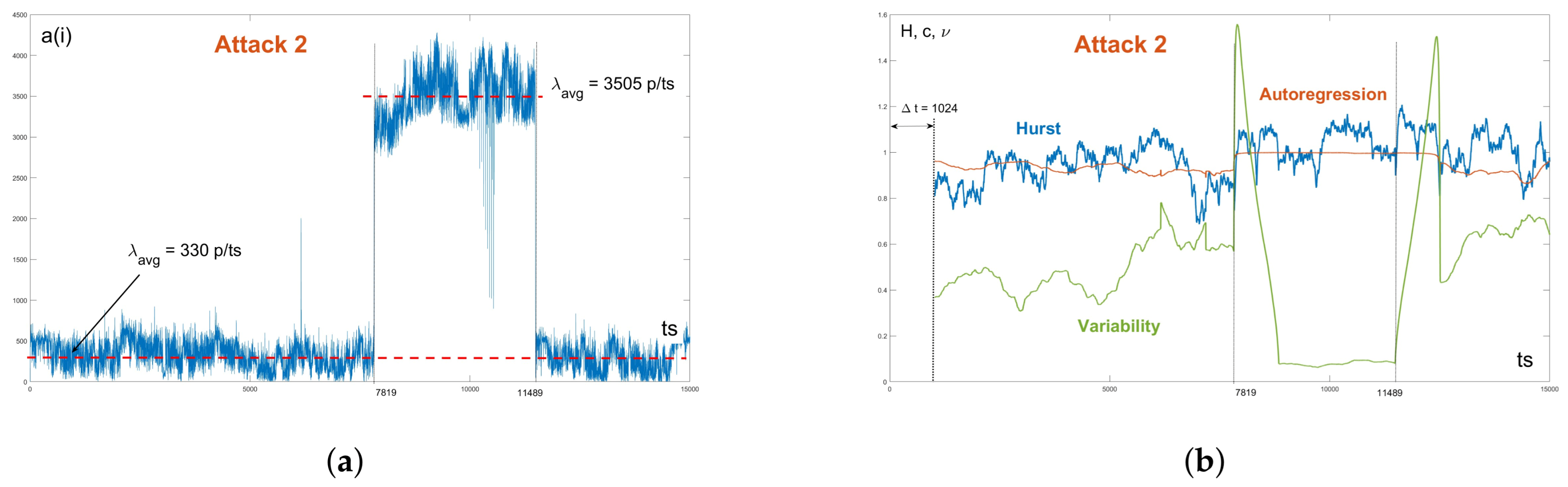
The second record (A2), which was also from ISCX 2012, was similar in structure to record R1, but the Hurst coefficient reacted minimally to the flood network traffic. The section was also 150 s long, with the attack occurring at 78.19 s as shown in Figure 17. The time slot was $ts=10\mathrm{ms}$. The normal IP traffic had an average rate of 33,000 p/s and the attack traffic had an average rate of 350,500 p/s.

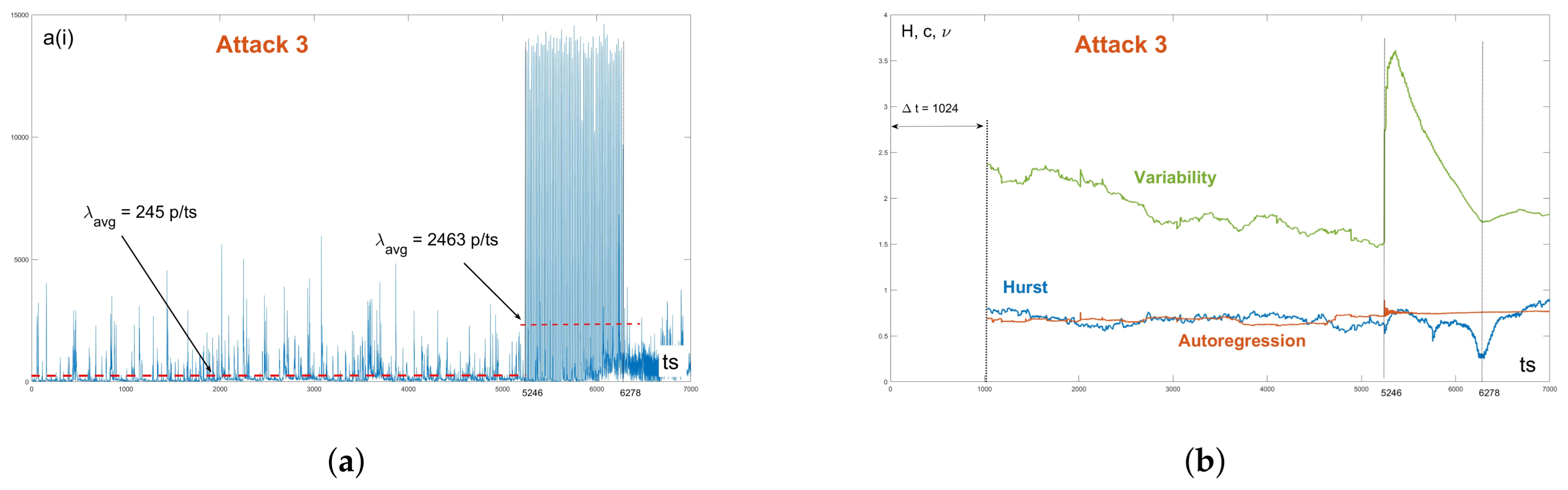
The third record (A3) was interesting in that the DDoS attack, instead of a bursty flow (as in A1 and A2), was made up of short attacks with a high intensity that quickly followed one another. The record was 70 s long, with the attack occurring in the 52th second and lasting 10 s (Figure 18). The time slot was also $ts=10\mathrm{ms}$. The normal IP traffic had an average rate of 2450 p/s and a peak rate of about 52,000 p/s. The attack traffic had average rate of only 24,630 p/s but the peak rate was very high at about 150,000 p/s, [52]. Even in this case, the Hurst coefficient did not react significantly.

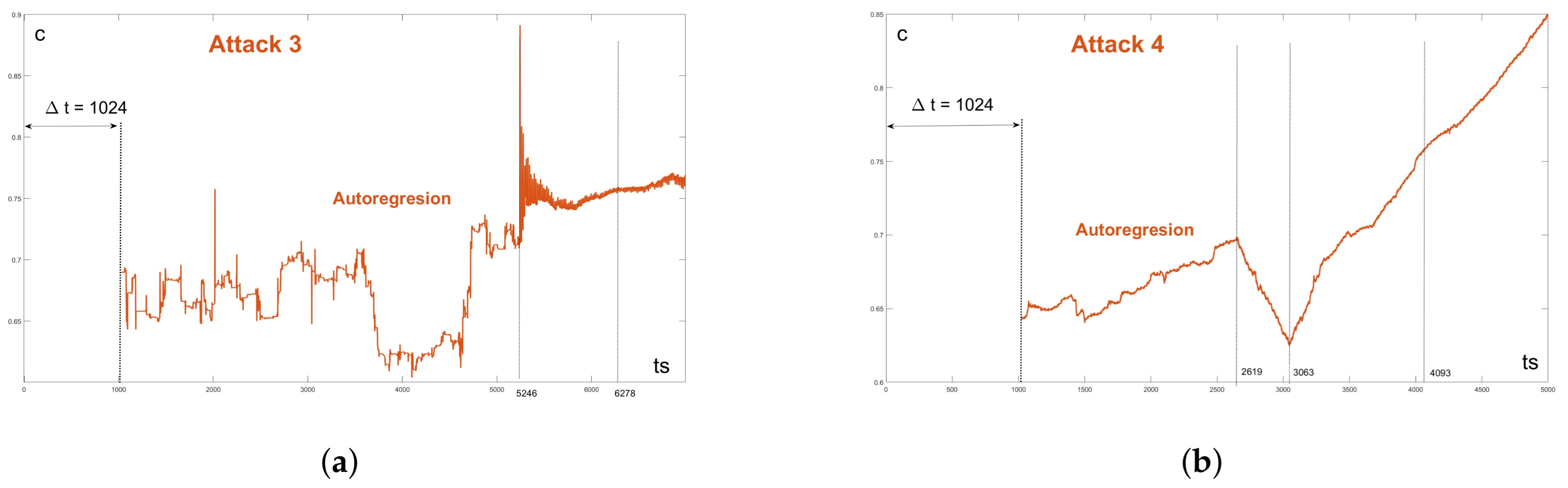
The fourth CICT attack represented a DDoS attack on the core server at the University of Žilina. Figure 19 shows the moment of the attack; the recording was 5 s long and according to the admin, the attack started at 3.063 s. The normal traffic had an average rate of 154 p/ms and the average rate of attack traffic was 267 p/s. The time slot was 1 ms.

The Hurst coefficient responded to the onset of the DDoS attack excellently, after approximately 30 milliseconds and reached significant values in 3.093 s. The autoregressive coefficient and coefficient of variation did not provide any recognizable values. Looking at the graphs of their values, however, we can see that both coefficients had a different course in the time interval from 2.619 s to 3.093 s. If we take a closer look at the attack record itself, you can really recognize the change in the structure of the flow as early as 2.619 s. We verified this opinion using the PCA method [53], which signaled an attack as early as 2.619 s [54].

In the previous figures, due to their small dispersion of values, the course of the coefficient of variation during the start of the network attack was hardly recognizable. Therefore, for all four attacks with AR(1), we present it in separate graphs, shown in Figure 20 and Figure 21.

We showed several diverse examples of DDoS attacks. During attacks A2 and A3, Hurst reacted minimally, the change in its behavior would be difficult to recognize, while the reactions of the parameter H during attacks A1 and A4 were expected to be standard. The coefficient of variation pleasantly surprised us. After experimenting with simulated scenarios, we expected that the change in the size of its values would correspond to an increase in the average rate. However, in the cases of A2 and A3, the coefficient strongly reacted to the onset of the attack. The autoregression coefficient noticeably reacted as well in the cases of A1 and A2; however, the reaction in A3 would be difficult to distinguish from the previous increase in normal operation.

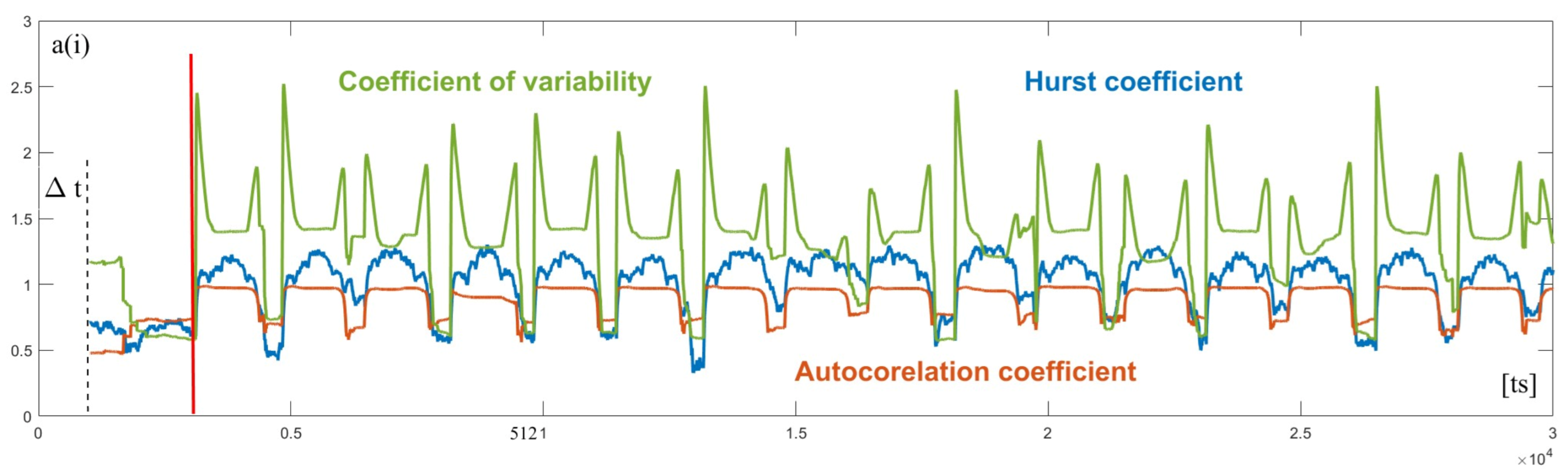
The fifth real record of an attack that we used for the purpose of experimentation is called CIC-IDS 2017 [55]. This is record of a cyclical DDoS attack. This record was created by the Canadian Institute for Cybersecurity and attacks were made from the Kali Linux operating system to the web server. The record consists of five flows from the working days of the week. Each day contains different types of attacks. For our experiments, we used a flow record from the Wednesday where the DDoS attack was recorded. For the experimentation, we chose a section 300 s long, and the attack occurred at the 31st second. The normal IP traffic had an average rate of 0.13 p/ms and a peak rate of 24 p/ms. During the attack, the average rate was 2.37 p/ms and the peak rate was 84 p/ms, see in Figure 22 and Figure 23. Since the average rate in the sliding window did not increase significantly when monitoring this flow, this type of attack is called a low-rate DDoS attack [56,57]:

During a cyclical DDoS attack, all three parameters were preserved as expected, they reacted roughly identically to short burst periods of the attack.

6. Symmetrically Predicting $\mathbf{\sigma }$-Tunnel

In the previous section, we saw on nonstandard samples of DDoS attacks how the selected coefficients reacted to the attack. However, our aim was to find a way for the computer (machine) to recognize these significant changes in the course of the time series of coefficient values. For the Hurst coefficient, in many cases, it would be sufficient to determine a reference value, e.g., 0.9, and if it was exceeded, the machine would report an attack. However, we showed that this method was not a rule and there were situations when the Hurst coefficient reacted minimally; therefore, we did not consider this method to be sufficiently robust.

Our effort consisted in finding a method by which the machine itself would detect a significant change in the values of the control coefficients. The main idea was to create a reference interval from the already-calculated coefficient values and then test whether the new coefficient value exceeded the interval limit. We called these intervals symmetrically predicting tunnels. There are different methods to create these tunnels. We chose one of the basic methods, $\sigma$-Tunnel, and denote it $\left[\sigma \text{-}\mathrm{T}\right]$.

As an example, we take the course of the Hurst parameter. The H values of the parameter that we want to use to create the control interval are denoted as $(h_1,h_2,\dots ,h_N)$. We call the predicted window (N length) the prediction window. From the $h_i$ values, we calculate average $\overline{H}$ and an estimation of standard deviation $\sigma$:

$$\overline{H}=\frac{1}{N}\sum _{i=1}^N{h}_i,\mathrm{and}\sigma =\sqrt{{\displaystyle \frac{1}{N-1}}\sum _{i=1}^N{\left(h_i-\overline{H}\right)}^2}$$

(21)

We create a symmetrical interval around average $\overline{H}$, $I=〈\overline{H}-n.\sigma ,\overline{H}+n.\sigma 〉$ and then test whether the new value of the Hurst parameter belongs to the predicting interval, $h_{N+1}\in I$. If it does not belong, the machine detects the beginning of the attack.

Based on experiments with real records, we decided to use an interval of length $2\sigma$. An interval with a length of $3\sigma$ is a standard in statistics, according to Chebyshev’s inequality, and it must contain at least 8/9 of all events [58]. However, the interval was able to adapt to the change in parameter values and there were no reports. Therefore, we decided to use the length $2\sigma$. According to Chebyshev’s inequality, at least $75\%$ of all events must be in the control interval. We denote such a predicting tunnel as $\left[2\sigma \text{-}T\right]$. Since we tested only one new value, $h_{N+1}$, the length of the predicting tunnel was 1. When testing different sizes of the predicting window on real records, we achieved the best results with the size $N=512\mathrm{ts}$, which was actually half the size of the used time window for calculating the coefficients ($\Delta t=1024\mathrm{ts}$). We therefore used the exact term for predicting tunnel $\left[2\sigma {\text{-}\mathrm{T}}_{512,1}\right]$. However, since we do not mention other settings in this work, we omit the indexes in the following. We present the use of the tunnel for the 1st and 4th attacks.

In Figure 24, we see that in both cases the values of the H parameter exceeded the upper limit of the control interval. However, we saw this reaction even during normal operation before an attack, with the difference that it lasted significantly shorter. These events were labeled as false alarms and the goal was to minimize them.

For a clear visualization of false reports and attack detection, we show in Figure 25 the difference between the upper limit of the predicting tunnel and the currently controlled value of the Hurst coefficient. Since in cases A1 and A2, the value of the Hurst coefficient increased, for the sake of clarity we did not show the situation between the lower limit and the parameter.

From other experiments, we selected the autoregression coefficient for Attack 2, see Figure 26, and the coefficient of variation for Attack 3, see Figure 27, to indicate the use of the predicting $\sigma$-tunnel.

The predicting tunnel captured a sudden increase or decrease in the values of the monitored parameters when a DDoS attack started or ended. In an effort to eliminate false reports, we first tried to smooth the parameter values. There were several possibilities but we used exponential smoothing [59]. It is a relatively simple method in which the values of the coefficient H are replaced by their weighted average according to the relationship:

$$S_1=h_1,S_i=\alpha ·h_{i-1}+(1-\alpha )·S_{i-1},i=2,3,\dots$$

(22)

We considered smoothing with the value $\alpha =0.1$ to be sufficient. At smaller values, there was already a significant shift in the moment of attack detection.

For an example of applying predicting tunnel $\left[2\sigma \text{-}\mathrm{T}\right]$ for the exponential smoothing of the detection parameter, we chose the Hurst coefficient for Attack 4, see Figure 28, and the autoregression coefficient for Attack 2, see Figure 29.

The exponential smoothing of the detection coefficients preserved the identification of the attack traffic and reduced the difference between the value of the coefficient and the interval limit for false reports, while the number of false reports decreased only minimally.

7. Results and Discussion

As we already mentioned in the introduction, our effort was to create an autonomous self-learning system of relatively simple software-implementable statistical methods for the purpose of a timely detection of DDoS attacks in a high-speed network infrastructure. Monitoring coefficients must record a change from standard to attack traffic by means of a significant change in their value. Subsequently, the monitoring probe must be able to recognize this change in the values of the coefficients of the newly loaded traffic using the previous development of the considered values.

We tested three different coefficients that described the probabilistic structure of the network flow. The tests were performed on simulated data using the MMRP process. We tested scenarios that simulated a standard bursty DDoS attack and a cyclical DDoS attack (low-rate DDoS). We conducted further tests on various real records of DDoS attacks. We presented five of the most interesting cases in this work.

In general, we can conclude that the Hurst reacted very well to a standard bursty DDoS attack; its values when processing standard traffic were mostly in the interval $〈0.4,0.6〉$; when the attack started, its values increased very quickly, within 2 to 5 ts, and they increased above $H>0.9$ or $H\to 1$. In many cases of real recording of network traffic, we could use $H=0.95$ as a reference value, but this was not always the rule. For some real samples, the H coefficient did not even reach the value of 0.9 or it did not react to the attack at all and behaved the same as during legitimate network traffic.

The coefficient of variation $\nu$ reacted on the simulated data similarly to the changing intensity of the average flow intensity ${\lambda }_{avg}$. This means that its reaction was significantly slower than that of the Hurst coefficient. However, in real records, the coefficient often reacted very quickly to a change in the flow’s character, although the parameter values ranged in the interval $〈0,\infty 〉$ according to the mean rate and variance of the flow. We performed experiments with the transformation of the coefficient using $V=exp(-\nu )$ into the interval $〈0,1〉$, but we did not obtain interesting results, so we did not mention these experiments. The way to teach a machine to recognize a DDoS attack using $\nu$ could be seen mainly in the use of a predicting $\sigma$-tunnel, or other predictions based on other mathematical methods.

The autoregression coefficient on simulated data also reacted significantly slower than the Hurst coefficient, but with real data, we often noticed a significant increase in values, even in cases where the Hurst coefficient did not react at all. The values of the AR(1) had a small variance, therefore the use of some reference value to recognize an attack was not possible, and to recognize an increase in values, for example, some predictive methods must be used.

The success of using the considered coefficients also depended on the length of the time window $\Delta t$, in which the values of the coefficients were calculated. In the presented experiments, we used $\Delta t=1024$ ts for the purpose of comparing AR(1) and the coefficient of variation with the Hurst coefficient. As the value of $\Delta t$ increased, the parameter values were smoothed out and the attack increased, but the computational complexity increased, especially with the H coefficient.

In addition to the detection of a DDoS attack, the coefficients applied to the IP traffic flow also provided us with information on the structure of individual parts of the flow, e.g., with A4, the AR(1) coefficient and the coefficient of variation recognized the change in flow earlier than the appropriate moment of the start of the attack as determined by the administrator.

In general, with experiments on real traffic capture, there is often a problem with obtaining a sufficiently long record of normal traffic. On a sufficiently long record, the prediction methods have time to more reliably calibrate the limits of the intervals permissible for the recognition of the flow anomaly.

The problem with obtaining a sufficient duration of normal traffic capture should not occur in practice, because we assume that after starting the monitoring probe, a sufficient duration of capture will contain the normal, nonattacking traffic.

8. Conclusions

In this article, we presented the use of three one-parameter statistical methods for detecting DDoS attacks: the Hurst coefficient, the autoregression coefficient and the coefficient of variation. Their success on simulated data was satisfactory, their application to real data was more interesting. The coefficients reacted differently on different data, and we presented the most interesting cases under the designations A1 to A4. In each case, at least one coefficient significantly increased or lowered its values. Unlike detection methods using, e.g., GAN networks, genetic algorithms, Bayes networks, PCA or other methods of machine learning with a teacher, the statistical coefficients mentioned above are computationally simple, easy to implement in software and do not require prior training with a teacher.

Although, as already stated, they mostly reacted visibly with their increase or decrease to the onset of the attack, it is necessary to teach the machine to recognize the changes that we see with the naked eye.

Therefore, in addition to examining other single-parametric methods, e.g., entropy, in our research, we focused on the creation of so-called prediction tunnels. We presented the first simple idea, the use of $\sigma$-tunnels, in this article. The method successfully recognized the onset of attacks on the given real data, but at the same time signaled several false reports. In an attempt to reduce the number of false reports, we applied exponential smoothing to the values of the coefficients. The recognition results only slightly improved. It is a challenge to create more effective predicting tunnels that would be less adaptable to sudden changes in parameter values. The use of multivariate regression, regression lines using boundary values of parameters, prediction using Fourier analysis, the use of neural network for prediction, etc., will be investigated in future work.

Of course, we will continue to deal with the testing of suitable one-parametric statistical coefficients, such as the skewness, kurtosis, various types of entropy, etc.