Dynamics Analysis of a Class of Stochastic SEIR Models with Saturation Incidence Rate

Abstract

In this article, a class of stochastic SEIR models with saturation incidence is studied. The model is a symmetric and compatible distribution family. This paper studies various properties of the system by constructing Lyapunov functions. First, the gradual properties of the systematic solution near the disease-free equilibrium of the deterministic model is studied, followed by the final behavior of the model, including stochastic persistence and final extinction. Finally, the existence conditions of the stationary distribution of the model are given, and then it is proved that it is traversed, and the corresponding conclusions are verified through numerical simulation.

1. Introduction

AIDS, hepatitis B and other infectious diseases affect people’s health, posing a great threat to physical and mental health, so the prediction and control of such infectious diseases is what we are pursuing. Through the study of infectious disease models, we can clearly understand the influence on the model of various factors, so that we can make good predictions about the occurrence of infectious disease, provide appropriate advice for government and public health department decision-making, and also provide scientific data for relevant departments. The study of infectious disease models has very important significance, so a correlation analysis of infectious disease models is conducted here.

In recent years, many scholars have engaged in research in infectious disease. Ezekiel et al. [1] studied the stability of a class of SIR models and numerical simulations, and interpretations of biological phenomena were performed using MATLAB software. Abdelaziz Mahmoud et al. [2] investigated the SIR model with a saturation treatment function. The paper analyzed the progressive stability of model equilibrium points, and also studied the long-term dynamic behavior of the system. Shihua Zhang et al. [3] analyzed the SIS model affected by age. This paper studied the local and global asymptotic stability of the disease-free and internal equilibrium points of the model. These scholars stated their own opinion on infectious disease models, these articles provided directions for the study of infectious disease. Although the stability of infectious disease models is important, we should also pay attention to other properties of infectious disease models, such as asymptotic properties, stationary distribution, etc., so it is necessary to study these in this paper.

After a virus invades a body, the virus will reproduce and grow, but the virus will not grow indefinitely. When it reaches a certain level, the infection will reach a saturation state, so it is necessary to add saturation incidence rate ${\displaystyle \frac{\beta SI}{1+\alpha I}}$ to the model, and it can be seen that when the infected population is large enough, the incidence rate reaches the saturation state. Related research should be specifically referred to in [4,5,6,7]. When the virus invades the human body, it does not immediately infect a person—it may lurk in our body for a period of time. This incubation time of different infectious diseases is different, so it is crucial to study the infectious disease model with the incubation period [8,9,10]. With the continuous research and cooperation of infectious disease models, a class of SEIR model with saturation incidence is proposed, as follows:

$$\left\{\begin{array}{cc}\hfill \frac{\mathrm{d}S\left(t\right)}{\mathrm{d}t}& =A-\frac{\beta S\left(t\right)I\left(t\right)}{1+\alpha I}-dS\left(t\right)\hfill \\ \hfill \frac{\mathrm{d}E\left(t\right)}{\mathrm{d}t}& =\frac{\beta S\left(t\right)I\left(t\right)}{1+\alpha I\left(t\right)}-(d+ϵ)E\left(t\right)\hfill \\ \hfill \frac{\mathrm{d}I\left(t\right)}{\mathrm{d}t}& =ϵE\left(t\right)-(d+u+v)I\left(t\right)\hfill \\ \hfill \frac{\mathrm{d}R\left(t\right)}{\mathrm{d}t}& =vI\left(t\right)-dR\left(t\right)\hfill \end{array}\right.$$

(1)

where $S\left(t\right),E\left(t\right),I\left(t\right)$ and $R\left(t\right)$ represent the numbers of easily infected, latent, infected, and recovered at time t, parameter A represents the constant input rate, $\alpha$ represents the saturation rate of the inhibitory effect, $\beta$ is the infection rate coefficient, d represents the natural mortality rate of the population, $ϵ$ is conversion rate from latent person to infected person, u is the disease mortality rate, and v is the natural recovery rate of the patient, all the parameters are positive numbers.

By observing the above formula, we see that the first three types of formula of the equation set do not involve $R\left(t\right)$. Therefore, we consider the following formula:

$$\left\{\begin{array}{cc}\hfill \frac{\mathrm{d}S\left(t\right)}{\mathrm{d}t}& =A-\frac{\beta S\left(t\right)I\left(t\right)}{1+\alpha I}-dS\left(t\right)\hfill \\ \hfill \frac{\mathrm{d}E\left(t\right)}{\mathrm{d}t}& =\frac{\beta S\left(t\right)I\left(t\right)}{1+\alpha I\left(t\right)}-(d+ϵ)E\left(t\right)\hfill \\ \hfill \frac{\mathrm{d}I\left(t\right)}{\mathrm{d}t}& =ϵE\left(t\right)-(d+u+v)I\left(t\right)\hfill \end{array}\right.$$

(2)

It calculates the disease-free equilibrium state $P_0=(\frac{d}{A},0,0)$ of system $\left(2\right)$, and $R_0=\frac{\beta Aϵ}{d(d+ϵ)(d+u+v)}$ is the basic reproduction number [11] of system $\left(2\right)$.

We often hear about the high-incidence season of infectious diseases. For example, measles is easiest spread in the population between spring and summer, influenza and mumps are most likely to appear in spring and fall, and bacterial dysentery often occurs in the summer and winter. Therefore, the spread of a virus is not only affected by the various factors above, but also by humidity, temperature and other environmental factors. Therefore, the above equation cannot adequately explain the real situation, as the research results may be different from the reality. Therefore, this paper studies the SEIR model with random perturbations [12,13,14]. If the random disturbance form of white noise [15,16] is in direct proportion to the $S\left(t\right)$, $E\left(t\right)$, and $I\left(t\right)$, then the above system of equations becomes

$$\left\{\begin{array}{cc}\hfill \mathrm{d}S\left(t\right)& =[A-\frac{\beta S\left(t\right)I\left(t\right)}{1+\alpha I}-dS\left(t\right)]\mathrm{d}t+{\sigma }_{1}S\left(t\right)\mathrm{d}{B}_1\left(t\right)\hfill \\ \hfill \mathrm{d}E\left(t\right)& =[\frac{\beta S\left(t\right)I\left(t\right)}{1+\alpha I\left(t\right)}-(d+ϵ)E\left(t\right)]\mathrm{d}t+{\sigma }_{2}E\left(t\right)\mathrm{d}{B}_2\left(t\right)\hfill \\ \hfill \mathrm{d}I\left(t\right)& =[ϵE\left(t\right)-(d+u+v)I\left(t\right)]\mathrm{d}t+{\sigma }_{3}I\left(t\right)\mathrm{d}{B}_3\left(t\right)\hfill \end{array}\right.$$

(3)

where $B_1\left(t\right),B_2\left(t\right)$ and $B_3\left(t\right)$ are Brownian motions [17,18] independent of each other, ${\sigma }_i$ is the intensity of Brownian motions $B_i\left(t\right)$, and ${\sigma }_i$ are all positive constants. $i=1,2,3$.

Brownian motion is a simple and symmetrical stochastic process on a straight line. Symmetry is an important property of Brownian motion. In studying stochastic differential equations, using symmetry methods can achieve simple problems, which facilitates the study of stochastic processes. Zhang N et al. [19] applied the symmetry method to backward stochastic differential equations and made important findings.

Infectious diseases have always threatened people’s physical and mental health and affected social stability. For the study of infectious disease, the stochastic model is more practical, and the stochastic method is more appropriate. For details, please refer to the literature [20]. Stochastic methods are also of great significance in computer science. Raza et al. [21] explained that when the threshold $C^{*}<1$, computer viruses are controlled. The authors made a significant contribution to computer protection by studying the dynamic behavior of computer viruses.

System $\left(3\right)$ is a system of stochastic differential equations. In the past few decades, many scholars have studied stochastic models, especially in biology [22,23,24,25,26,27]. Compared with deterministic systems, stochastic differential equations are relatively difficult to study. We study the problem according to the Ito formula [28] and stochastic analysis.

The main content of this article is divided into three parts. The first part mainly analyzes the orbital stability [29,30] of the model, the second part analyzes the final behavior of infectious, including long-lasting and ultimate extinction, and the third part discusses the ergodicity of the stochastic system.

Compared with past articles, this paper has some advantages in terms of the model. Zhang et al. [31] did not consider the effects of random perturbations. The role of latency was not considered by Rajasekar et al. [32]. Faranda et al. [33] did not consider the role of incidence rate. This paper comprehensively considers the influence of many factors such as saturation, latency and random perturbation, and the past articles only consider one or two of these factors; therefore, this model is more complicated and difficult to study. This paper has some advantages in proving the process of stationary distribution, compared with Han et al. [34], whose paper constructs multiple Lyapunov functions [35,36,37] that are complex in form and relatively difficult to understand. However, we construct a Lyapunov function using the method of minimum value of function, and then, according to the Ito formula, obtain the $L{V}_4$ and divide $L{V}_4$ into multiple functions. Finally, we discuss the problem according to the idea of classification and limit. The demonstration process is very clear and rigorous, so the methods are much more interesting and easier to understand.

The Lyapunov function method plays an important role in studying the stability of the system. Because the stationary distribution is also the weak stability of the stochastic system, it is effective to use the Lyapunov function method to study the asymptotic stability and stationary distribution of the system. To prove the stochastic persistence and final extinction of the model, auxiliary functions are constructed, and then a rigorous and rational mathematical derivation is carried out. The method is used properly, and the proof is clear, so the method is appropriate. The paper also verifies the correctness of the conclusion using numerical simulation.

The main content of this article is divided into four sections. In the first section, when the basic reproduction number $R_0<1$ of deterministic system $\left(2\right)$, we discuss the progressive properties of the stochastic system by constructing an auxiliary function, and analyze the asymptotic behavior of solutions of the stochastic system near the disease-free equilibrium point of its deterministic system. In the second section, we study the final situation of the model solution, and discuss the conditions for the stochastic persistence and final extinction of system $\left(3\right)$. Through proof of the theorem, it is found that the size of the random perturbation coefficient ${\sigma }_i(i=1,2,3)$ is of great significance in controlling the occurrence of disease, and this conclusion is verified by the numerical simulation. In the third section, the paper studies the ergodicity of system $\left(3\right)$. The article proves that system $\left(3\right)$ has a unique stationary distribution [38,39,40] when the system parameters satisfy certain conditions, and the correctness of the conclusion is verified by numerical simulation. Section 4 summarizes the full text and suggests an outlook.

2. The Gradual Progression of the Solution near Disease-Free Equilibrium State of the Deterministic System

When $R_0<1$, system $\left(2\right)$ exists in a disease-free equilibrium state $P_0=(\frac{d}{A},0,0)$, and has global stability. Obviously, $P_0$ is not a solution to system $\left(3\right)$, so is there any rule in the solution of system $\left(3\right)$ around $P_0$? Relevant studies are followed in this section.

Theorem 1. 

If $R_0<1$, and the following conditions are met

$$\begin{array}{c}\hfill m_1=d-{\sigma }_1^2-\frac{\beta }{2\alpha }-\frac{A\beta }{2d}>0,\\ \hfill m_2=d+ϵ-\frac{{\sigma }_2^2}{2}-\frac{\beta }{2\alpha }-\frac{ϵ}{2}>0,\\ \hfill m_3=d+u+v-\frac{{\sigma }_3^2}{2}-\frac{A\beta }{2d}-\frac{ϵ}{2}>0\end{array}$$

(4)

then for any initial value condition $(S\left(0\right),E\left(0\right),I\left(0\right))\in R_{+}^3$, the solution of system $\left(3\right)$ has the following properties:

$$\underset{t\to \infty }{lim}sup\frac{1}{t}·E{\int }_0^t[{(S-\frac{A}{d})}^2+E^2+I^2]\mathrm{d}s\le \frac{\frac{{\sigma }_1^2{A}^2}{d^2}+c_{1}A}{m_1\wedge m_2\wedge m_3}$$

$c_1$ is a positive number, which will be given later.

Proof of Theorem 1. 

First, we define a Lyapunov function $V_1=\frac{1}{2}{(S-\frac{A}{d})}^2+\frac{1}{2}{E}^2+\frac{1}{2}{I}^2+c_{1}S+c_{2}E+c_{3}I=V_{11}+V_{12}+V_{13}+V_{14}$, where $V_{11}=\frac{1}{2}{(S-\frac{A}{d})}^2+\frac{1}{2}{E}^2+\frac{1}{2}{I}^2,V_{12}=c_{1}S,V_{13}=c_{2}E,V_{14}=c_{3}I$, all $c_i(i=1,2,3)$ are normal numbers, and clearly $V_1$ is $R_3^{+}\to R^{+}$, according to the Ito formula (See Appendix A)

$$\begin{array}{c}\hfill \mathrm{d}{V}_1=L{V}_1\mathrm{d}t+{\sigma }_{1}S(S-\frac{A}{d}+c_1)\mathrm{d}{B}_1+{\sigma }_{2}E(E+c_2)\mathrm{d}{B}_2+{\sigma }_{3}I(I+c_3)\mathrm{d}{B}_1\end{array}$$

(5)

where

$$\begin{array}{cc}\hfill L{V}_{11}=& (S-\frac{A}{d})(A-\frac{\beta SI}{1+\alpha I}-dS)+E(\frac{\beta SI}{1+\alpha I}-(d+ϵ)E)+I(ϵE-(d+u+v)I)\hfill \\ \hfill & +\frac{{\sigma }_1^2{S}^2}{2}+\frac{{\sigma }_2^2{E}^2}{2}+\frac{{\sigma }_3^2{I}^2}{2}\hfill \\ \hfill =& -d{(S-\frac{A}{d})}^2-\frac{\beta SI}{1+\alpha I}(S-\frac{A}{d})+\frac{\beta SI}{1+\alpha I}E-(d+ϵ)E^2+ϵEI-(d+u+v)I^2\hfill \\ \hfill & +\frac{{\sigma }_1^2{S}^2}{2}+\frac{{\sigma }_2^2{E}^2}{2}+\frac{{\sigma }_3^2{I}^2}{2}\hfill \\ \hfill \le & -d{(S-\frac{A}{d})}^2+\frac{A}{d}\beta SI+\frac{\beta SE}{\alpha }-(d+ϵ)E^2+ϵEI-(d+u+v)I^2+{\sigma }_1^2{(S-\frac{A}{d})}^2\hfill \\ \hfill & +{\sigma }_1^2\frac{A^2}{d^2}+\frac{{\sigma }_2^2{E}^2}{2}+\frac{{\sigma }_3^2{I}^2}{2}\hfill \\ \hfill =& -(d-{\sigma }_1^2){(S-\frac{A}{d})}^2-(d+ϵ-\frac{{\sigma }_2^2}{2})E^2-(d+u+v-\frac{{\sigma }_3^2}{2})I^2+\frac{A\beta }{d}SI+\frac{\beta SE}{\alpha }+ϵEI\hfill \\ \hfill & +{\sigma }_1^2\frac{A^2}{d^2}\hfill \\ \hfill =& -(d-{\sigma }_1^2){(S-\frac{A}{d})}^2-(d+ϵ-\frac{{\sigma }_2^2}{2})E^2-(d+u+v-\frac{{\sigma }_3^2}{2})I^2\hfill \\ \hfill & +\frac{A\beta }{d}(S-\frac{A}{d})I+\frac{\beta }{\alpha }(S-{\displaystyle \frac{A}{d}})E+ϵEI+\frac{A^2\beta }{d^2}I+\frac{\beta A}{\alpha d}E+{\sigma }_1^2\frac{A^2}{d^2}\hfill \end{array}$$

(6)

$$\begin{array}{c}\hfill L{V}_{12}=c_1(A-\frac{\beta SI}{1+\alpha I}-dS)=c_{1}A-\frac{c_1\beta SI}{1+\alpha I}-c_{1}dS\end{array}$$

(7)

$$L{V}_{13}=c_2[\frac{\beta SI}{1+\alpha I}-(d+ϵ)E]=\frac{c_2\beta SI}{1+\alpha I}-c_2(d+ϵ)E$$

(8)

$$L{V}_{14}=c_3(ϵE-(d+u+v)I)=c_3ϵE-c_3(d+u+v)I$$

(9)

Take $c_1=c_2$, bring $\left(6\right),\left(7\right),\left(8\right)$ and $\left(9\right)$ into $\left(5\right)$

$$\begin{array}{cc}\hfill L{V}_1\le & -(d-{\sigma }_1^2){(S-\frac{A}{d})}^2-(d+ϵ-\frac{{\sigma }_2^2}{2})E^2-(d+u+v-\frac{{\sigma }_3^2}{2})I^2+\frac{A\beta }{d}(S-\frac{A}{d})I+\frac{\beta }{\alpha }(S-{\displaystyle \frac{A}{d}})E\hfill \\ \hfill & +ϵEI+\frac{A^2\beta }{d^2}I+\frac{\beta A}{\alpha d}E+c_{1}A-c_2(d+ϵ)E+c_3ϵE-c_3(d+u+v)I+{\sigma }_1^2\frac{A^2}{d^2}\hfill \\ \hfill =& -(d-{\sigma }_1^2){(S-\frac{A}{d})}^2-(d+ϵ-\frac{{\sigma }_2^2}{2})E^2-(d+u+v-\frac{{\sigma }_3^2}{2})I^2+\frac{A\beta }{d}(S-\frac{A}{d})I+\frac{\beta }{\alpha }(S-{\displaystyle \frac{A}{d}})E\hfill \\ \hfill & +ϵEI+(\frac{\beta A}{\alpha d}-c_2(d+ϵ)+c_3ϵ)E+(\frac{A^2\beta }{d^2}-c_3(d+u+v))I+c_{1}A+{\sigma }_1^2\frac{A^2}{d^2}\hfill \end{array}$$

(10)

let $c_3=\frac{A^2\beta }{d^2(d+u+v)}$, $c_2=\frac{\beta A}{ad(d+ϵ)}+\frac{A^2\beta ϵ}{d^2(d+u+v)(d+ϵ)}$, so $c_j$ satisfy the following conditions, $j=2,3$.

$$\begin{array}{c}\hfill \frac{\beta A}{\alpha d}-c_2(d+ϵ)+c_3ϵ=0,\frac{A^2\beta }{d^2}-c_3(d+u+v)=0\end{array}$$

(11)

according to the basic inequality has

$$(S-\frac{A}{d})I\le \frac{1}{2}{(S-\frac{A}{d})}^2+\frac{1}{2}{I}^2,(S-\frac{A}{d})E\le \frac{1}{2}{(S-\frac{A}{d})}^2+\frac{1}{2}{E}^2,EI\le \frac{E^2}{2}+\frac{I^2}{2}$$

(12)

bring $(11)$ and $(12)$ into $(10)$

$$\begin{array}{cc}\hfill L{V}_1\le & -(d-{\sigma }_1^2-\frac{\beta }{2\alpha }-\frac{A\beta }{2d}){(S-\frac{A}{d})}^2-(d+ϵ-\frac{{\sigma }_2^2}{2}-\frac{\beta }{2\alpha }-\frac{ϵ}{2})E^2-(d+u+v-\frac{{\sigma }_3^2}{2}-\frac{A\beta }{2d}-\frac{ϵ}{2})I^2\hfill \\ & +{\sigma }_1^2\frac{A^2}{d^2}+c_{1}A\hfill \\ \hfill =& -m_1{(S-\frac{A}{d})}^2-m_2{E}^2-m_3{I}^2+{\sigma }_1^2\frac{A^2}{d^2}+c_{1}A\hfill \end{array}$$

(13)

where $m_1=d-{\sigma }_1^2-\frac{\beta }{2\alpha }-\frac{A\beta }{2d},m_2=d+ϵ-\frac{{\sigma }_2^2}{2}-\frac{\beta }{2\alpha }-\frac{ϵ}{2},m_3=d+u+v-\frac{{\sigma }_3^2}{2}-\frac{A\beta }{2d}-\frac{ϵ}{2}$, bring $(13)$ into the $(5)$, both sides simultaneously integrate and take the expectation

$$\begin{array}{cc}{V}_1(S\left(t\right),E\left(t\right),I\left(t\right))=& E{\int }_0^t[-m_1{(S-\frac{A}{d})}^2-m_2{E}^2-m_3{I}^2]\mathrm{d}s+V_1(S\left(0\right),E\left(0\right),I\left(0\right))+({\sigma }_1^2\frac{A^2}{d^2}+c_{1}A)t\hfill \end{array}$$

then both sides are simultaneously divided by the time t, and take the limit to t, sorting out

$$\underset{t\to \infty }{lim}sup\frac{1}{t}·E{\int }_0^t[{(S-\frac{A}{d})}^2+E^2+I^2]\mathrm{d}s\le \frac{\frac{{\sigma }_1^2{A}^2}{d^2}+c_{1}A}{m_1\wedge m_2\wedge m_3}$$

□

This theorem indicates that the solution of system $\left(3\right)$ vibrates randomly around the disease-free equilibrium point $P_0$ of system $\left(2\right)$. When the perturbation strength ${\sigma }_i$ is smaller, the smaller vibration amplitude is found, and the more likely the solution of system $\left(3\right)$ is to approach a disease-free equilibrium state of the deterministic system.

3. The Final Behavior of the Infectious Disease

We can know the conditions of system $\left(2\right)$ from the basic reproduction number, including the long-term existence or extinction of the disease. Under what conditions does system $\left(3\right)$ persist or become extinct? Next, this section will focus on the persistence and demise of the disease of system $\left(3\right)$.

Definition 1. 

If $\underset{t\to \infty }{lim}\frac{1}{t}{\int }_0^{t}f\left(s\right)\mathrm{d}s>0$, it represents $f\left(s\right)$ stochastic persistence.

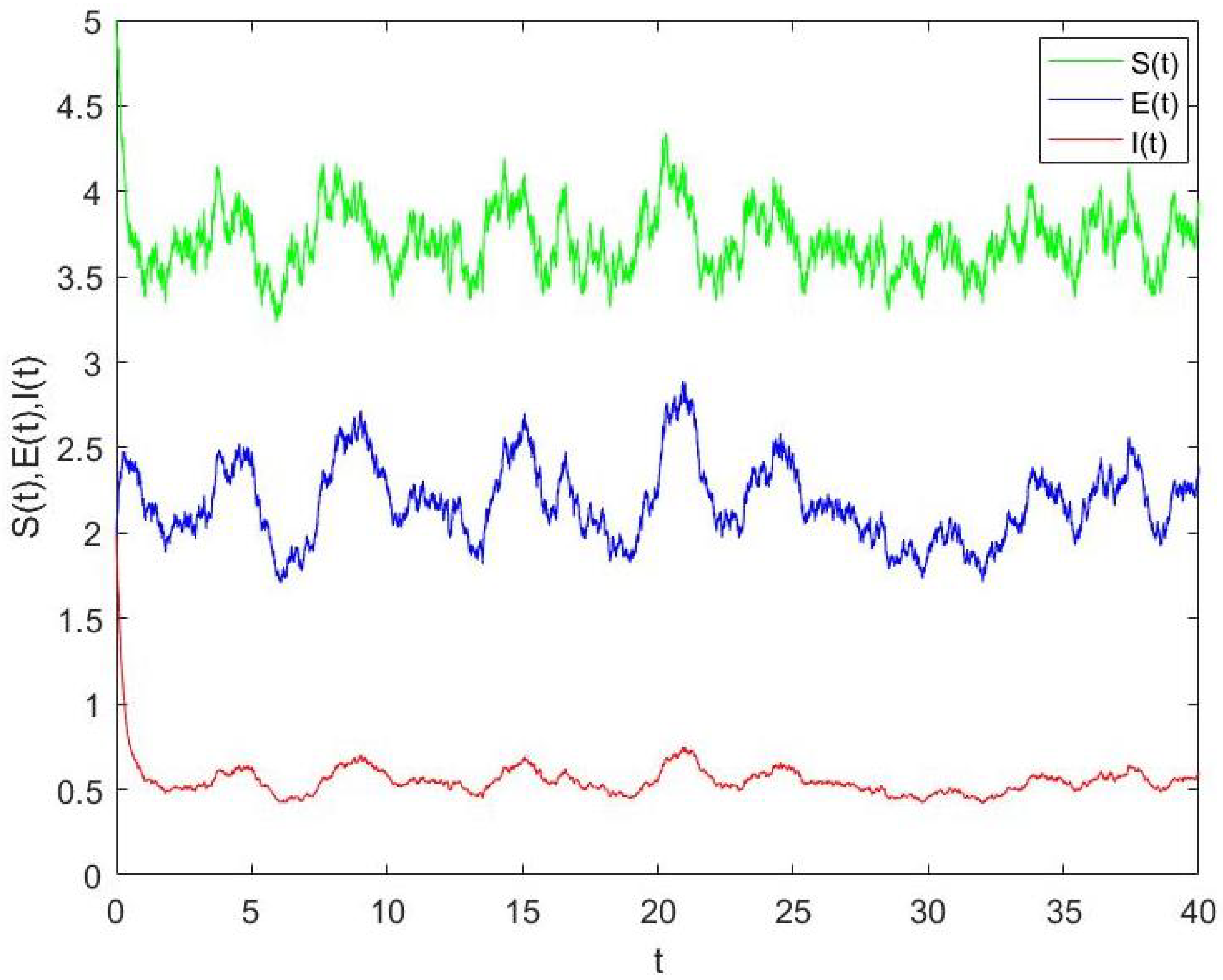
3.1. The Infected Person Persists

Theorem 2. 

If $3\sqrt[3]{A\beta ϵ}-\gamma >0$, γ is a positive number, and will be given later. For any initial condition $\left(S\right(0),E(0),I(0\left)\right)$, the infected person will persist, and the solution of system $\left(3\right)$ satisfies the following conclusions:

$$\begin{array}{cc}\hfill \underset{t\to \infty }{lim}\frac{1}{t}{\int }_0^{t}S\left(s\right)\mathrm{d}s& >\frac{\alpha (d+ϵ)(3\sqrt[3]{A\beta ϵ}-\gamma )(d+u+v)}{[\beta +\alpha (d+u+v\left)\right]ϵ\beta }\hfill \\ \hfill \underset{t\to \infty }{lim}\frac{1}{t}{\int }_0^{t}E\left(s\right)\mathrm{d}s& >\frac{(3\sqrt[3]{A\beta ϵ}-\gamma )(d+u+v)}{[\beta +\alpha (d+u+v\left)\right]ϵ}\hfill \\ \hfill \underset{t\to \infty }{lim}\frac{1}{t}{\int }_0^{t}I\left(s\right)\mathrm{d}s& >\frac{3\sqrt[3]{A\beta ϵ}-\gamma }{\beta +\alpha (d+u+v)}\hfill \end{array}$$

(14)

Proof of Theorem 2. 

First, we define a function $V_2(S,E,I)=-lnS-lnE-lnI$, according to the Ito formula:

$$\mathrm{d}{V}_2\left(t\right)=L{V}_2\left(t\right)\mathrm{d}t-{\sigma }_1\mathrm{d}{B}_1\left(t\right)-{\sigma }_2\mathrm{d}{B}_2\left(t\right)-{\sigma }_3\mathrm{d}{B}_3\left(t\right)$$

(15)

where

$$\begin{array}{cc}\hfill L{V}_2\left(t\right)=& -\frac{1}{S}(A-\frac{\beta SI}{1+\alpha I}-dS)-\frac{1}{E}(\frac{\beta SI}{1+\alpha I}-(d+ϵ)E)-\frac{1}{I}(ϵE-(d+u+v)I)-\frac{1}{2}({\sigma }_1^2+{\sigma }_2^2+{\sigma }_3^2)\hfill \\ \hfill =& -\frac{A}{S}+\frac{\beta I}{1+\alpha I}+d-\frac{\beta SI}{E(1+\alpha I)}+(d+ϵ)-\frac{ϵE}{I}+(d+u+v)-\frac{1}{2}({\sigma }_1^2+{\sigma }_2^2+{\sigma }_3^2)\hfill \\ \hfill \le & -\frac{A}{S}-\frac{\beta SI}{E(1+\alpha I)}-\frac{ϵE(1+\alpha I)}{I}+\alpha ϵE+\beta I+\gamma \hfill \\ \hfill \le & -3\sqrt[3]{A\beta ϵ}+\gamma +\alpha ϵE+\beta I\hfill \end{array}$$

(16)

where $\gamma =(3d+u+v+ϵ)-\frac{1}{2}({\sigma }_1^2+{\sigma }_2^2+{\sigma }_3^2)$, bring $\left(16\right)$ into $\left(15\right)$, take the integration in the interval $(0,t)$, then both sides are simultaneously divided by t, and take the limit to t.

$$\begin{array}{cc}\hfill 0\le & -3\sqrt[3]{A\beta ϵ}+\gamma +\underset{t\to \infty }{lim}\frac{\beta }{t}{\int }_0^{t}I\left(s\right)\mathrm{d}s+\underset{t\to \infty }{lim}\frac{\alpha ϵ}{t}{\int }_0^{t}E\left(s\right)\mathrm{d}s\hfill \\ \hfill & -\underset{t\to \infty }{lim}\frac{1}{t}{\int }_0^t{\sigma }_1\mathrm{d}{B}_1\left(s\right)-\underset{t\to \infty }{lim}\frac{1}{t}{\int }_0^t{\sigma }_2\mathrm{d}{B}_2\left(s\right)-\underset{t\to \infty }{lim}\frac{1}{t}{\int }_0^t{\sigma }_3\mathrm{d}{B}_3\left(s\right)\hfill \end{array}$$

(17)

according to the powerful number law of a martingale

$$\underset{t\to \infty }{lim}\frac{1}{t}{\int }_0^t{\sigma }_1\mathrm{d}{B}_1\left(s\right)=\underset{t\to \infty }{lim}\frac{1}{t}{\int }_0^t{\sigma }_2\mathrm{d}{B}_2\left(s\right)=\underset{t\to \infty }{lim}\frac{1}{t}{\int }_0^t{\sigma }_3\mathrm{d}{B}_3\left(s\right)=0$$

so $\left(17\right)$ becomes

$$\underset{t\to \infty }{lim}\frac{\beta }{t}{\int }_0^{t}I\left(s\right)\mathrm{d}s+\underset{t\to \infty }{lim}\frac{\alpha ϵ}{t}{\int }_0^{t}E\left(s\right)\mathrm{d}s\ge 3\sqrt[3]{A\beta ϵ}-\gamma$$

(18)

According to the third formula of system $\left(3\right)$, take the integration in the interval $(0,t)$.

$$I\left(t\right)-I\left(0\right)={\int }_0^t[ϵE\left(s\right)-(d+u+v)I\left(s\right)]\mathrm{d}s+{\int }_0^t{\sigma }_{3}I\left(s\right)\mathrm{d}{B}_3\left(s\right)$$

both sides are simultaneously divided by t, and take the limit to t.

$$\underset{t\to \infty }{lim}\frac{d+u+v}{t}{\int }_0^{t}I\left(s\right)\mathrm{d}s=\underset{t\to \infty }{lim}\frac{ϵ}{t}{\int }_0^{t}E\left(s\right)\mathrm{d}s+\underset{t\to \infty }{lim}\frac{1}{t}{\int }_0^t{\sigma }_{3}I\left(s\right)\mathrm{d}B\left(s\right)$$

(19)

according to the powerful number law of a martingale

$$\underset{t\to \infty }{lim}\frac{1}{t}{\int }_0^t{\sigma }_{3}I\left(s\right)\mathrm{d}B\left(s\right)=0$$

so $\left(19\right)$ becomes

$$\underset{t\to \infty }{lim}\frac{d+u+v}{t}{\int }_0^{t}I\left(s\right)\mathrm{d}s=\underset{t\to \infty }{lim}\frac{ϵ}{t}{\int }_0^{t}E\left(s\right)\mathrm{d}s$$

sorting out

$$\underset{t\to \infty }{lim}\frac{1}{t}{\int }_0^{t}E\left(s\right)\mathrm{d}s=\underset{t\to \infty }{lim}\frac{d+u+v}{ϵ}·\frac{1}{t}{\int }_0^{t}I\left(s\right)\mathrm{d}s$$

(20)

bring $\left(20\right)$ into $\left(18\right)$, sorting out

$$\underset{t\to \infty }{lim}\frac{1}{t}{\int }_0^{t}I\left(s\right)\mathrm{d}s>\frac{3\sqrt[3]{A\beta ϵ}-\gamma }{\beta +\alpha (d+u+v)}$$

according to Formula $\left(20\right)$

$$\underset{t\to \infty }{lim}\frac{1}{t}{\int }_0^{t}E\left(s\right)\mathrm{d}s>\frac{(3\sqrt[3]{A\beta ϵ}-\gamma )(d+u+v)}{[\beta +\alpha (d+u+v\left)\right]ϵ}$$

(21)

according to the second formula sub of system $\left(3\right)$

$$\mathrm{d}E\le [\frac{\beta }{\alpha }S-(d+ϵ)E]\mathrm{d}t+{\sigma }_{2}E\mathrm{d}{B}_2\left(t\right)$$

both sides integrate in the interval $(0,t)$, then, divided by t and taken the limit, the following results are obtained

$$\underset{t\to \infty }{lim}\frac{1}{t}{\int }_0^{t}S\left(s\right)\mathrm{d}s>\frac{(d+ϵ)\alpha (3\sqrt[3]{A\beta ϵ}-\gamma )(d+u+v)}{[\beta +\alpha (d+u+v\left)\right]ϵ\beta }$$

(22)

□

Theorem 2 shows that when the parameters meet the corresponding conditions, the infectious disease will persist, and the smaller the random disturbance coefficient ${\sigma }_i$ (i = 1, 2, 3) and the greater the constant input rate A, the more likely it is that the infectious disease will persist.

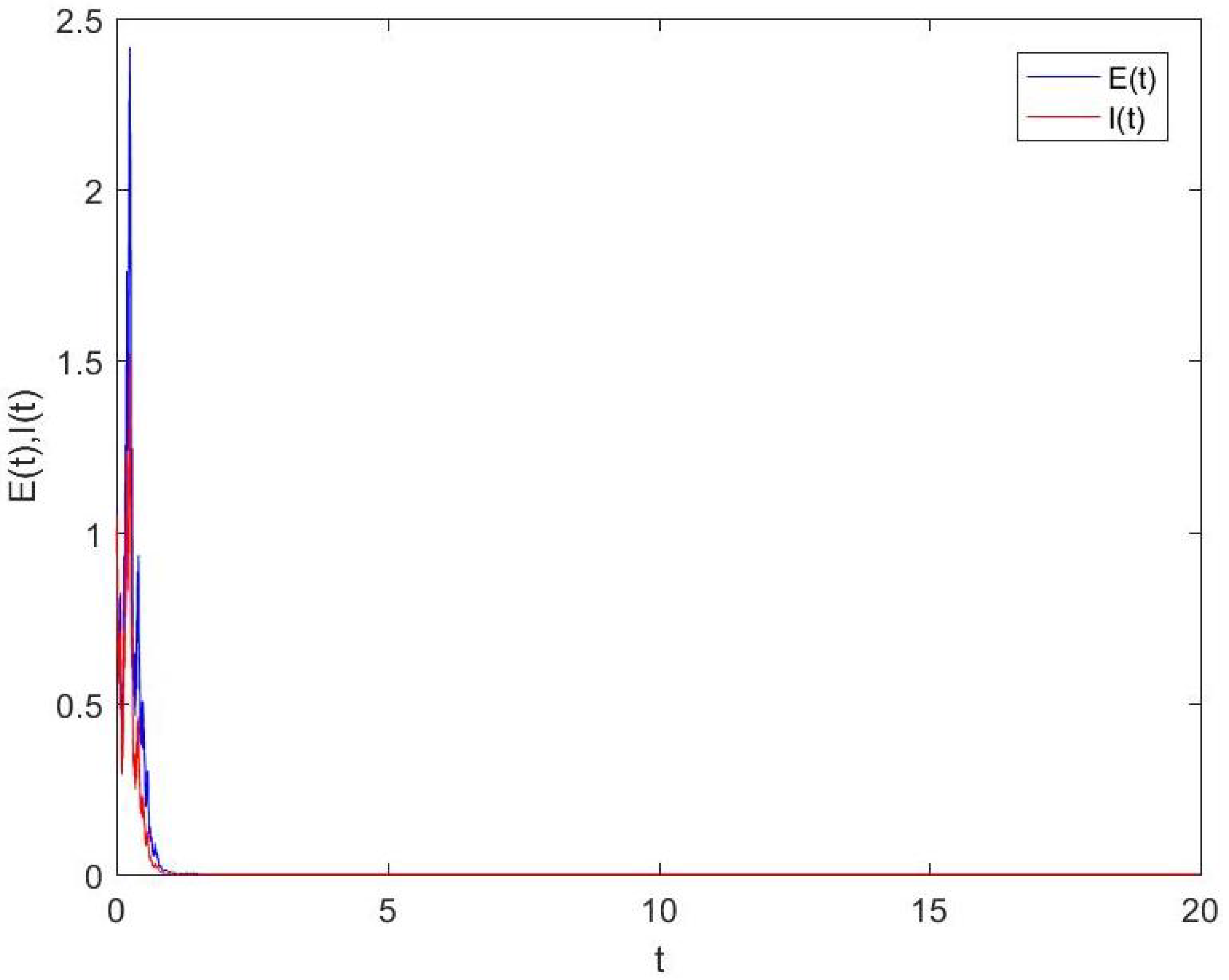
3.2. Extermination of Infectious Diseases

Theorem 2 gives a sufficient condition for the persistence of infectious disease. So, what conditions can the parameters meet to make the disease extinct? To achieve the elimination of infectious disease, a correlational study is discussed next in the section.

Theorem 3. 

If $\beta \frac{A}{d}-\frac{h}{2}<0$, where $h=min\{d+\frac{{\sigma }_2^2}{2},(d+u+v)+\frac{{\sigma }_3^2}{2}\}$, for any initial value condition, the latent and infected person will perish, and the infectious disease will be under control.

Proof of Theorem 3. 

Define a function $V_3=ln(E+I)$, according to the Ito formula

$$\mathrm{d}{V}_3\left(t\right)=L{V}_3\left(t\right)\mathrm{d}t+\frac{{\sigma }_{2}E}{E+I}\mathrm{d}{B}_2\left(t\right)+\frac{{\sigma }_{3}I}{E+I}\mathrm{d}{B}_3\left(t\right)$$

(23)

where

$$\begin{array}{cc}\hfill L{V}_3=& \frac{1}{E+I}[\frac{\beta SI}{1+\alpha I}-(d+ϵ)E+ϵE-(d+u+v)I]-\frac{{\sigma }_2^2{E}^2+{\sigma }_3^2{I}^2}{2{(E+I)}^2}\hfill \\ \hfill =& \frac{\frac{\beta SI}{1+\alpha I}}{E+I}+\frac{(-d-\frac{{\sigma }_2^2}{2})E^2+[-(d+u+v)-\frac{{\sigma }_3^2}{2}]I^2-(2d+u+v)EI}{{(E+I)}^2}\hfill \\ \hfill \le & \beta S+\frac{(-d-\frac{{\sigma }_2^2}{2})E^2+[-(d+u+v)-\frac{{\sigma }_3^2}{2}]I^2}{{(E+I)}^2}\hfill \\ \hfill \le & \beta S-\frac{(d+\frac{{\sigma }_2^2}{2})E^2+[(d+u+v)+\frac{{\sigma }_3^2}{2}]I^2}{2(E^2+I^2)}\hfill \\ \hfill \le & \beta S-\frac{h}{2}\hfill \end{array}$$

(24)

where $h=min\{d+\frac{{\sigma }_2^2}{2},(d+u+v)+\frac{{\sigma }_3^2}{2}\}$, bring $\left(24\right)$ into $\left(23\right)$, take the integration in the interval $(0,t)$, then divide both sides by t simultaneously, and take the limit, sorting out

$$\underset{t\to \infty }{lim}\frac{ln(E+I)}{t}\le \underset{t\to \infty }{lim}\beta ·\frac{1}{t}{\int }_0^{t}S\left(s\right)\mathrm{d}s-\frac{h}{2}$$

(25)

According to system $\left(3\right)$, the two sides will sum simultaneously

$$\mathrm{d}(S+E+I)=[A-d(S+E+I)-(u+v)I]\mathrm{d}t+{\sigma }_{1}S\mathrm{d}{B}_1+{\sigma }_{2}E\mathrm{d}{B}_2+{\sigma }_{3}I\mathrm{d}{B}_3$$

integrate in interval $(0,t)$, then divide both sides by t simultaneously, and take the limit.

$$0\le A-\underset{t\to \infty }{lim}\frac{d}{t}{\int }_0^t(S\left(s\right)+E\left(s\right)+I\left(s\right))\mathrm{d}s$$

so there is the following conclusion

$$\underset{t\to \infty }{lim}\frac{1}{t}{\int }_0^{t}S\left(s\right)\mathrm{d}s\le \frac{A}{d}$$

(26)

Bring $\left(26\right)$ into $\left(25\right)$

$$\underset{t\to \infty }{lim}\frac{ln(E+I)}{t}\le \frac{\beta A}{d}-\frac{h}{2}<0$$

so there is a result

$$\underset{t\to \infty }{lim}E\left(s\right)=\underset{t\to \infty }{lim}I\left(s\right)=0$$

□

Theorem 3 shows that the purpose of controlling infectious disease can be achieved by controlling the size of the parameters, and the smaller the constant input rate A or the larger the perturbation coefficient ${\sigma }_2$ and ${\sigma }_3$, the more likely it is to control the condition.

3.3. Numerical Simulation

The Euler method [41] and the Milstein method [42,43] are formally simple numerical simulation methods. The Milstein method has a higher convergence order compared to the Euler method, so the numerical solution is closer to the real solution. To verify the correctness of the above conclusions, this section conducts numerical simulations to verify the conclusion using the Milstein method. The expression is as follows:

$$\left\{\begin{array}{cc}\hfill S_{i+1}& =S_i+(A-\frac{\beta S_i{I}_i}{1+\alpha I_i}-d{S}_i)\Delta t+{\sigma }_1{S}_i\sqrt{\Delta t}{\xi }_1+\frac{1}{2}{\sigma }_1^2{S}_i({\xi }_1^2-1)\Delta t\hfill \\ \hfill E_{i+1}& =E_i+(\frac{\beta S_i{I}_i}{1+\alpha I_i}-(d+ϵ)E_i)\Delta t+{\sigma }_2{E}_i\sqrt{\Delta t}{\xi }_2+\frac{1}{2}{\sigma }_2^2{E}_i({\xi }_2^2-1)\Delta t\hfill \\ I_{i+1}& =I_i+(ϵE_i-(d+u+v)E_i)\Delta t+{\sigma }_3{I}_i\sqrt{\Delta t}{\xi }_3+\frac{1}{2}{\sigma }_3^2{I}_i({\xi }_3^2-1)\Delta t\hfill \end{array}\right.$$

Theorem 2 proves a sufficient condition for disease persistence. Taking the parameter $S\left(0\right)=5,E\left(0\right)=I\left(0\right)=2,\Delta t=\frac{80}{2^{16}},A=8,\beta =8,\alpha =2,ϵ=1,{\sigma }_1=0.1,{\sigma }_2=0.1,{\sigma }_3=0.1,$$ϵ=1,d=1,u=2,v=1$, so $3\sqrt[3]{8\times 8\times 1}-[(3\times 1+2+1+1)+\frac{1}{2}(0.1^2+0.1^2+0.1^2)]=5.015>0$ satisfies the Theorem 2 condition, and the numerical simulation result is shown in Figure 1.

Theorem 3 gives sufficient conditions for the extinction of infectious disease. Taking the parameters $E\left(0\right)=1,I\left(0\right)=1,\Delta t=\frac{80}{2^{16}},A=4,\beta =1,\alpha =3,ϵ=1,{\sigma }_1=2,{\sigma }_2=2,$${\sigma }_3=2,$$d=4,u=2,v=2$, so $1\times \frac{4}{4}-\frac{1}{2}min\{4+\frac{4}{2},4+2+2+\frac{4}{2}\}=-2<0$, and the numerical simulation result is shown in Figure 2.

4. Stationary Distribution

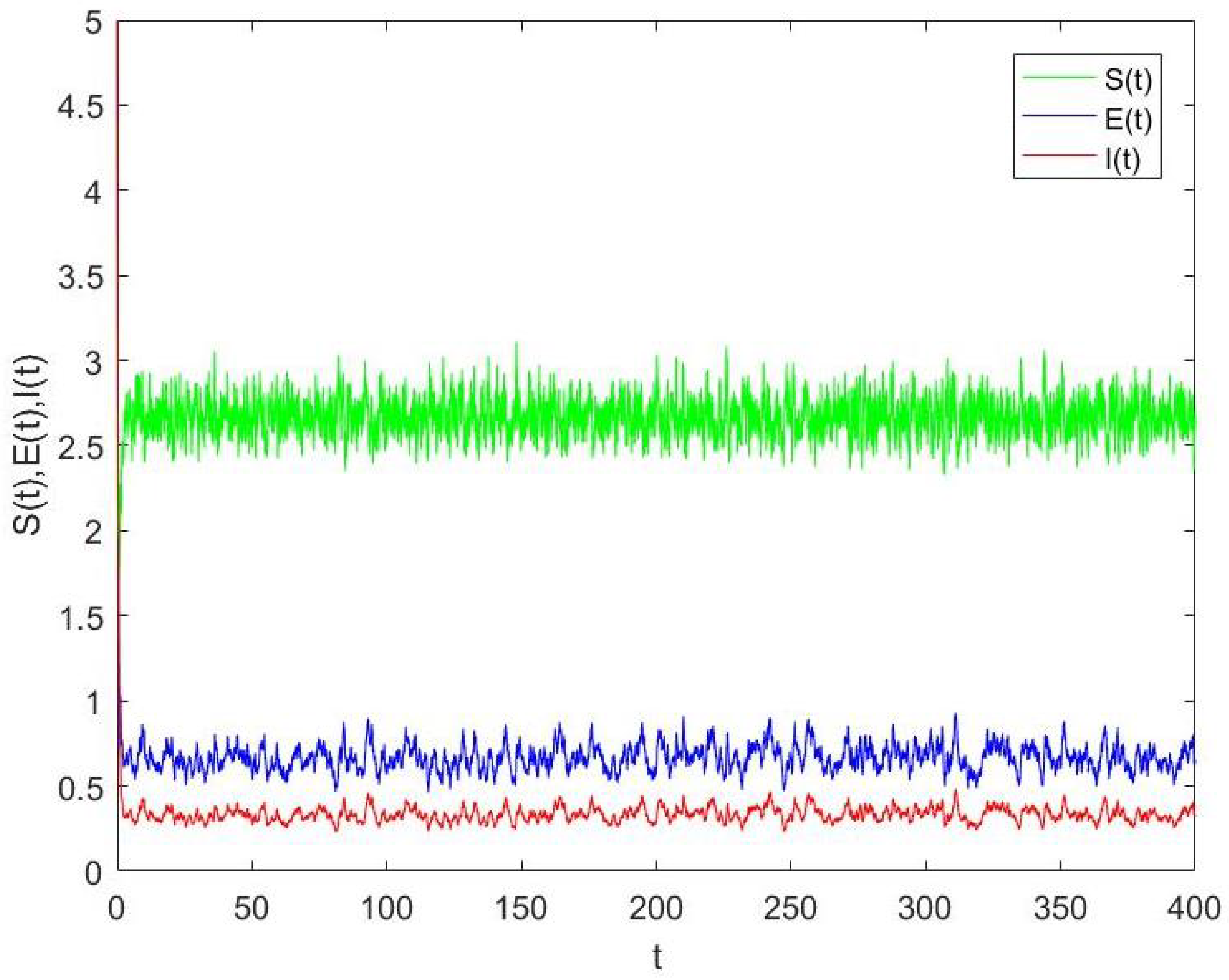
4.1. The Stationary Distribution and Its Ergodicity

Stationary distribution plays a crucial role in the study of stochastic infectious disease models, which can indicate an otherwise qualitatively invariant probability distribution. By analyzing stationary distribution and the ergodicity of the model, we can obtain a good grasp of the model. Then, we are able to predict the change regulation of infectious disease. Relevant study is conducted in this section.

stipulate: $\check{f}=su{p}_{x\in R}f\left(x\right),\widehat{f}=in{f}_{x\in R}f\left(x\right)$

Theorem 4. 

If $B=d-\frac{1}{2}({\sigma }_1^2\vee {\sigma }_2^2\vee {\sigma }_3^2)>0$, and $-3\sqrt[3]{A\beta ϵ}+3d+u+v+ϵ+\frac{\beta }{\alpha }+\frac{{\sigma }_1^2}{2}+\frac{{\sigma }_2^2}{2}+\frac{{\sigma }_3^2}{2}<0$, for any initial value condition $(S\left(0\right),E\left(0\right),I\left(0\right))\in R_{+}^3$, system $\left(3\right)$ has a unique stationary distribution, and this distribution is ergodic.

Proof of Theorem 4. 

First, we consider the function $\widetilde{V_4}=\frac{1}{1+\theta }{(S+E+I)}^{1+\theta }+M(-lnS-lnE-lnI-{\lambda }_{1}I)-lnS-lnE=V_{41}+M(V_{42}+V_{43})+V_{44}$, where $V_{41}=\frac{1}{1+\theta }{(S+E+I)}^{1+\theta },V_{42}=-lnS-lnE-lnI,V_{43}=-{\lambda }_{1}I,V_{44}=-lnS-lnE$, ${\lambda }_1$ is a pending positive number, we clearly know that $\widetilde{V_4}$ has a minimum value of $V_{40}$.

Thus, we define a Lyapunov function $V_4=\widetilde{V_4}-V_{40}$, obviously $R_3^{+}\to R^{+}$, according to the Ito formula

$$\begin{array}{cc}\hfill L{V}_{41}=& {(S+E+I)}^{\theta }[A-dS-dE-(d+u+v)I]+\frac{\theta }{2}{(S+E+I)}^{\theta -1}{\sigma }_1^2{S}^2\hfill \\ \hfill & +\frac{\theta }{2}{(S+E+I)}^{\theta -1}{\sigma }_2^2{E}^2+\frac{\theta }{2}{(S+E+I)}^{\theta -1}{\sigma }_3^2{I}^2\hfill \\ \hfill \le & A{(S+E+I)}^{\theta }-d{(S+E+I)}^{1+\theta }+\frac{\theta }{2}{(S+E+I)}^{1+\theta }({\sigma }_1^2\vee {\sigma }_2^2\vee {\sigma }_3^2)\hfill \\ \hfill =& A{(S+E+I)}^{\theta }-(d-\frac{\theta }{2}({\sigma }_1^2\vee {\sigma }_2^2\vee {\sigma }_3^2)){(S+E+I)}^{1+\theta }\hfill \\ \hfill \le & H-\frac{B}{2}{(S+E+I)}^{1+\theta }\hfill \end{array}$$

(27)

where $H=su{p}_{t\in (0,\infty )}A{(S+E+I)}^{\theta }-\frac{B}{2}{(S+E+I)}^{1+\theta },B=d-\frac{\theta }{2}({\sigma }_1^2\vee {\sigma }_2^2\vee {\sigma }_3^2)$

$$\begin{array}{cc}\hfill L{V}_{42}=& -\frac{1}{S}(A-\frac{\beta SI}{1+\alpha I}-dS)-\frac{1}{E}(\frac{\beta SI}{1+\alpha I}-(d+ϵ)E)-\frac{1}{I}[ϵE-(d+u+v)I]+{\displaystyle \frac{{\sigma }_1^2}{2}}+{\displaystyle \frac{{\sigma }_2^2}{2}}+{\displaystyle \frac{{\sigma }_3^2}{2}}\hfill \\ \hfill =& -\frac{A}{S}+\frac{\beta I}{1+\alpha I}+d-\frac{\beta SI}{E(1+\alpha I)}+(d+ϵ)-\frac{ϵE(1+\alpha I)}{I}+(d+u+v)+{\displaystyle \frac{{\sigma }_1^2}{2}}+{\displaystyle \frac{{\sigma }_2^2}{2}}+{\displaystyle \frac{{\sigma }_3^2}{2}}+ϵ\alpha E\hfill \\ \hfill \le & -3\sqrt[3]{A\beta ϵ}+\frac{\beta }{\alpha }+3d+ϵ+u+v+{\displaystyle \frac{{\sigma }_1^2}{2}}+{\displaystyle \frac{{\sigma }_2^2}{2}}+{\displaystyle \frac{{\sigma }_3^2}{2}}+ϵ\alpha E\hfill \\ \hfill =& -\eta +ϵ\alpha E\hfill \end{array}$$

(28)

where $\eta =3\sqrt[3]{A\beta ϵ}-\frac{\beta }{\alpha }-3d-ϵ-u-v-{\displaystyle \frac{{\sigma }_1^2}{2}}-{\displaystyle \frac{{\sigma }_2^2}{2}}-{\displaystyle \frac{{\sigma }_3^2}{2}}>0$

$$\begin{array}{c}\hfill L{V}_{43}=-{\lambda }_1[ϵE-(d+u+v)I]=-{\lambda }_1ϵE+{\lambda }_1(d+u+v)I\end{array}$$

(29)

$$\begin{array}{cc}\hfill L{V}_{44}=& -\frac{1}{S}(A-\frac{\beta SI}{1+\alpha I}-dS)-\frac{1}{E}[\frac{\beta SI}{1+\alpha I}-(d+ϵ)E]+\frac{1}{2}{\sigma }_1^2+\frac{1}{2}{\sigma }_2^2\hfill \\ \hfill =& -\frac{A}{S}+\frac{\beta I}{1+\alpha I}+d-\frac{\beta SI}{E(1+\alpha I)}+(d+ϵ)+\frac{1}{2}{\sigma }_1^2+\frac{1}{2}{\sigma }_2^2\hfill \end{array}$$

(30)

let ${\lambda }_1=\alpha$, comprehensive $\left(27\right),\left(28\right),\left(29\right),\left(30\right)$, there is a following result

$$\begin{array}{cc}\hfill L{V}_4\le & H-\frac{B}{2}{(S+E+I)}^{1+\theta }+M(-\eta +\alpha (d+u+v)I)-\frac{A}{S}+\frac{\beta I}{1+\alpha I}+d\hfill \\ & -\frac{\beta SI}{E(1+\alpha I)}+(d+ϵ)+\frac{1}{2}{\sigma }_1^2+\frac{1}{2}{\sigma }_2^2\hfill \end{array}$$

let $F=H+\frac{\beta }{\alpha }+d+(d+ϵ)+\frac{1}{2}{\sigma }_1^2+\frac{1}{2}{\sigma }_2^2$

$$L{V}_4\le f_1\left(S\right)+f_2\left(E\right)+f_3\left(I\right)-\frac{\beta SI}{E(1+\alpha I)}$$

where $f_1\left(S\right)=F-\frac{B}{2}{S}^{\theta +1}-\frac{A}{S},f_2\left(E\right)=-\frac{B}{2}{E}^{\theta +1},f_3\left(I\right)=-{\displaystyle \frac{B}{2}}{I}^{\theta +1}+M(-\eta +\alpha (d+u+v)I)$, consider the following bounded set

$$U=\{(S,E,I)\in R_{+}^3,{ϵ}_1\le S\le \frac{1}{{ϵ}_1},{ϵ}_2\le E\le \frac{1}{{ϵ}_2},{ϵ}_3\le I\le \frac{1}{{ϵ}_3}\}$$

${ϵ}_1,{ϵ}_2$ and ${ϵ}_3$ are all arbitrarily small quantities, such that

$$D=R_{+}^3\backslash U=U_1\cup U_2\cup U_3\cup U_4\cup U_5\cup U_6$$

where

$$\begin{array}{c}\hfill U_1=\{(S,E,I)\in R_{+}^3,S<{ϵ}_1\}{U}_2=\{(S,E,I)\in R_{+}^3,S>\frac{1}{{ϵ}_1}\}\\ \hfill U_3=\{(S,E,I)\in R_{+}^3,E<{ϵ}_2\}{U}_4=\{(S,E,I)\in R_{+}^3,E>\frac{1}{{ϵ}_2}\}\\ U_5=\{(S,E,I)\in R_{+}^3,I<{ϵ}_3\}{U}_6=\{(S,E,I)\in R_{+}^3,I>\frac{1}{{ϵ}_3}\}\end{array}$$

Case 1: when $(S,E,I)\in U_1$

$$L{V}_4\le F-\frac{A}{S}+\check{f_3}<-1$$

Case 2: when $(S,E,I)\in U_2$

$$L{V}_4\le F-\frac{B}{2}{S}^{1+\theta }+\check{f_3}<-1$$

Case 3: when $(S,E,I)\in U_5$, take M is large enough to make the following result valid

$$L{V}_4\le \check{f_1}-M\eta <-1$$

Case 4: when $(S,E,I)\in U_6$.

$$L{V}_4\le \check{f_1}-\frac{B}{2}{I}^{1+\theta }+M(-\eta +\alpha (d+u+v)I)<-1$$

Case 5: when $(S,E,I)\in U_3$, there are two more cases. The first type of S or I tends to zero, which is the same as in case 1 and case 3 above. We shall not discuss this any further; we mainly observe that neither S nor I tends to zero.

$$L{V}_4\le \check{f_1}+\check{f_3}-\frac{\beta SI}{E(1+\alpha I)}<-1$$

Case 6: when $(S,E,I)\in U_6$.

$$L{V}_4\le \check{f_1}-\frac{B}{2}{E}^{1+\theta }+\check{f_3}<-1$$

In summary, the six cases always hold for $L{V}_4<-1$ in set D. Then, we consider the diffusion matrix of system $\left(3\right)$

$$C_{3\times 3}=\left[\begin{array}{ccc}{\sigma }_1^2{S}^2& 0& 0\\ 0& {\sigma }_2^2{E}^2& 0\\ 0& 0& {\sigma }_3^2{I}^2\end{array}\right]$$

select $N=min\{{\sigma }_1^2{S}^2,{\sigma }_2^2{E}^2,{\sigma }_3^2{I}^2\}$, so there is

$$\begin{array}{c}\hfill \sum _{i,j=1}^3(\sum _{k=1}^3)a_{ik}(S,E,I)a_{jk}(S,E,I)){\psi }_i{\psi }_j{\psi }_k={\sigma }_1^2{S}^2{\psi }_1^2+{\sigma }_2^2{E}^2{\psi }_2^2+{\sigma }_3^2{I}^2{\psi }_3^2\ge N{\parallel \psi \parallel }^2\end{array}$$

(31)

In summary, system $\left(3\right)$ has a unique stationary distribution, and this stationary distribution is ergodic. (See Appendix B). □

Theorem 4 shows that when the parameters meet the corresponding conditions, system $\left(3\right)$ will have a unique traversal stationary distribution, i.e., the system will fluctuate up and down around a fixed point.

4.2. Numerical Simulation

Theorem 4 proves sufficient conditions for stationary distribution, taking the parameters $S\left(0\right)=E\left(0\right)=I\left(0\right)=5,A=8,\beta =4,ϵ=2,{\sigma }_1=0.1,{\sigma }_2=0.1,{\sigma }_3=0.1,d=2,u=1,$$v=1,\alpha =1$. Numerical simulation results are shown in Figure 3.

5. Conclusions

In this paper, we present the SEIR model with saturation incidence through a certain background, find the system has some limitations, and then improve the model. Stochastic perturbations are added to the model to make the model more realistic. For stochastic systems, the paper is divided into three parts to study the properties of the model.

In the first part, we study the gradual progression of the stochastic system, when the basic reproduction number of the deterministic system $R_0<1$. We mainly discuss the gradual progression of the model near the disease-free equilibrium state of its deterministic system.

In the second part, we study the long-term dynamic behavior of the system, mainly analyzing the final behavior of the model. The stochastic persistence and extinction of the system has very important practical significance. We study the conditions for stochastic persistence and extinction by constructing auxiliary functions, and give numerical simulation results of the theorem. From the conclusion $3\sqrt[3]{A\beta ϵ}-\gamma >0$ of Theorem 2, we know that the smaller the random perturbation coefficient ${\sigma }_i(i=1,2,3)$, the more likely the disease is to persist. According to conclusion $\beta \frac{A}{d}-\frac{h}{2}<0$ of Theorem 3, the disease is more likely to become extinct when the random perturbation coefficients ${\sigma }_2$ and ${\sigma }_3$ are larger. Therefore, the outbreak of the disease can be controlled by reasonably controlling the size of the random disturbance coefficient.

In the final part, we prove the sufficient conditions for the existence of a stationary distribution, and give corresponding numerical simulations. According to the conclusion of Theorem 4, when the random perturbation coefficient is small enough, and parameter D is reasonably controlled, stochastic model $\left(3\right)$ has a unique stationary distribution, and is ergodic. The application of stationary distribution in infectious disease is particularly important. By studying the stationary distribution of the system, we can know the overall trend of the system, and have a good grasp of infectious disease, so that we can take the most appropriate measure to deal with the occurrence of disease.

However, the model still has some limitations. This paper only considers the impact of white noise on the model, and does not think about the impact of Levy noise. In addition, a viral invasion into a body will not immediately produce an effect, and the paper did not consider any time-delay effect. In the future learning process, learning content and knowledge structure will be updated so that better progress can be made.

References

1. Ezekiel, D.; Iyase, S.A.; Anake, T.A. Stability Analysis of an SIR Infectious Disease Model. In Proceedings of the 2nd International Conference on Recent Trends in Applied Research (ICoRTAR 2021), Virtual, 8–9 October 2021. [Google Scholar]
2. Abdelaziz, M.A.M.; Ismail, A.I.; Abdullah, F.A.; Mohd, M.H. Discrete-Time Fractional Order SIR Epidemic Model with Saturated Treatment Function. Int. J. Nonlinear Sci. Numer. Simul. 2020, 21, 397–424. [Google Scholar] [CrossRef]
3. Zhang, S.; Xu, R. Global Stability of an SIS Epidemic Model with Age of Vaccination. Differ. Equ. Dyn. Syst. 2022, 30, 1–22. [Google Scholar] [CrossRef]
4. Kaddar, A. Stability analysis in a delayed SIR epidemic model with a saturated incidence rate. Nonlinear Anal. Model. Control. 2010, 3, 299–306. [Google Scholar] [CrossRef]
5. Xu, C.; Yu, Y.; Ren, G. Dynamic analysis of a stochastic predator–prey model with Crowley–Martin functional response, disease in predator, and saturation incidence. J. Comput. Nonlinear Dyn. 2020, 15, 071004. [Google Scholar] [CrossRef]
6. Shatanawi, W.; Arif, M.S.; Raza, A.; Rafiq, M.; Bibi, M.; Abbasi, J.N. Structure-Preserving Dynamics of Stochastic Epidemic Model with the Saturated Incidence Rate. Comput. Mater. Contin. 2020, 64, 797–811. [Google Scholar] [CrossRef]
7. Liu, C.; Cui, R. Qualitative analysis on an SIRS reaction–diffusion epidemic model with saturation infection mechanism. Nonlinear Anal. Real World Appl. 2021, 62, 103364. [Google Scholar] [CrossRef]
8. Liu, Z.; Magal, P.; Seydi, O.; Webb, G. A COVID-19 epidemic model with latency period. Infect. Dis. Model. 2020, 5, 323–337. [Google Scholar] [CrossRef]
9. Zhang, L.; Wang, Z.C.; Zhao, X.Q. Threshold dynamics of a time periodic reaction–diffusion epidemic model with latent period. J. Differ. Equ. 2015, 258, 3011–3036. [Google Scholar] [CrossRef]
10. Liu, X.; Wang, Y.; Zhao, X.Q. Dynamics of a climate-based periodic Chikungunya model with incubation period. Appl. Math. Model. 2020, 80, 151–168. [Google Scholar] [CrossRef]
11. Dietz, K. The estimation of the basic reproduction number for infectious diseases. Stat. Methods Med. Res. 1993, 2, 23–41. [Google Scholar] [CrossRef]
12. Wang, Y.; Jiang, D.; Hayat, T.; Alsaedi, A. Stationary distribution of an HIV model with general nonlinear incidence rate and stochastic perturbations. J. Frankl. Inst. 2019, 356, 6610–6637. [Google Scholar] [CrossRef]
13. Liu, Q.; Kan, B.; Wang, Q.; Fang, Y. Cluster synchronization of Markovian switching complex networks with hybrid couplings and stochastic perturbations. Phys. Stat. Mech. Its Appl. 2019, 526, 120937. [Google Scholar] [CrossRef]
14. Zeb, A.; Kumar, S.; Tesfay, A.; Kumar, A. A stability analysis on a smoking model with stochastic perturbation. Int. J. Numer. Methods Heat Fluid Flow 2021, 32, 915–930. [Google Scholar] [CrossRef]
15. Allen, J.C.; Hobbs, S.L. Spectral estimation of non-stationary white noise. J. Frankl. Inst. 1997, 334, 99–116. [Google Scholar] [CrossRef]
16. Allen, E.J.; Novosel, S.J.; Zhang, Z. Finite element and difference approximation of some linear stochastic partial differential equations. Stoch. Int. J. Probab. Stoch. Process. 1998, 64, 117–142. [Google Scholar] [CrossRef]
17. Funaki, T.; Gao, Y.; Hilhorst, D. Existence and uniqueness of the entropy solution of a stochastic conservation law with a Q-Brownian motion. Math. Methods Appl. Sci. 2020, 43, 5860–5886. [Google Scholar] [CrossRef]
18. Prakasa Rao, B.L.S. Parametric inference for stochastic differential equations driven by a mixed fractional Brownian motion with random effects based on discrete observations. Stoch. Anal. Appl. 2022, 40, 236–245. [Google Scholar] [CrossRef]
19. Zhang, N.; Jia, G. W-symmetries of backward stochastic differential equations, preservation of simple symmetries and Kozlov’s theory. Commun. Nonlinear Sci. Numer. Simul. 2021, 93, 105527. [Google Scholar] [CrossRef]
20. Raza, A.; Rafiq, M.; Baleanu, D.; Shoaib Arif, M.; Naveed, M.; Ashraf, K. Competitive numerical analysis for stochastic HIV/AIDS epidemic model in a two-sex population. IET Syst. Biol. 2019, 13, 305–315. [Google Scholar] [CrossRef]
21. Raza, A.; Arif, M.S.; Rafiq, M.; Bibi, M.; Naveed, M.; Iqbal, M.U.; Butt, Z.; Naseem, H.A.; Abbasi, J.N. Numerical treatment for stochastic computer virus model. Comput. Model. Eng. Sci. 2019, 120, 445–465. [Google Scholar] [CrossRef]
22. Briat, C.; Khammash, M. Robust and structural ergodicity analysis of stochastic biomolecular networks involving synthetic antithetic integral controllers. IFAC-PapersOnLine 2017, 50, 10918–10923. [Google Scholar] [CrossRef]
23. Bachar, M.; Batzel, J.; Ditlevsen, S. Stochastic Biomathematical Models; Springer: Berlin/Heidelberg, Germany, 2012. [Google Scholar]
24. Kazeroonian, A.; Theis, F.J.; Hasenauer, J. Modeling of stochastic biological processes with non-polynomial propensities using non-central conditional moment equation. IFAC Proc. Vol. 2014, 47, 1729–1735. [Google Scholar] [CrossRef] [Green Version]
25. Jorge, J. On the average dynamical behaviour of stochastic population models. IFAC Proc. Vol. 2014, 47, 5270–5275. [Google Scholar]
26. Hening, A.; Tran, K.Q. Harvesting and seeding of stochastic populations: Analysis and numerical approximation. J. Math. Biol. 2020, 81, 65–112. [Google Scholar] [CrossRef] [PubMed]
27. Zhang, X.; Li, W.; Liu, M.; Wang, K. Dynamics of a stochastic Holling II one-predator two-prey system with jumps. Phys. Stat. Mech. Its Appl. 2015, 421, 571–582. [Google Scholar] [CrossRef]
28. Catuogno, P.; Olivera, C. Time-dependent tempered generalized functions and Itô’s formula. Appl. Anal. 2014, 93, 539–550. [Google Scholar] [CrossRef] [Green Version]
29. Li, J. Orbital Stability of Peakons for the Modified Camassa—Holm Equation. Acta Math. Sin. Engl. Ser. 2022, 38, 148–160. [Google Scholar] [CrossRef]
30. Fu, T.; Wang, Y. Orbital stability around the primary of a binary asteroid system. J. Guid. Control Dyn. 2021, 44, 1607–1620. [Google Scholar] [CrossRef]
31. Zhang, T.; Teng, Z. Pulse vaccination delayed SEIRS epidemic model with saturation incidence. Appl. Math. Model. 2008, 32, 1403–1416. [Google Scholar] [CrossRef]
32. Rajasekar, S.P.; Pitchaimani, M.; Zhu, Q. Dynamic threshold probe of stochastic SIR model with saturated incidence rate and saturated treatment function. Phys. Stat. Mech. Its Appl. 2019, 535, 122300. [Google Scholar] [CrossRef]
33. Faranda, D.; Alberti, T. Modeling the second wave of COVID-19 infections in France and Italy via a stochastic SEIR model. Chaos Interdiscip. J. Nonlinear Sci. 2020, 30, 111101. [Google Scholar] [CrossRef] [PubMed]
34. Han, B.; Jiang, D.; Hayat, T.; Alsaedi, A.; Ahmad, B. Stationary distribution and extinction of a stochastic staged progression AIDS model with staged treatment and second-order perturbation. Chaos Solitons Fractals 2020, 140, 110238. [Google Scholar] [CrossRef] [PubMed]
35. Liu, L.; Liu, Y.J.; Chen, A.; Tong, S.; Chen, C.L. Integral barrier Lyapunov function-based adaptive control for switched nonlinear systems. Sci. China Inf. Sci. 2020, 63, 1–14. [Google Scholar] [CrossRef] [Green Version]
36. Cao, W.; Zhu, Q. Razumikhin-type theorem for pth exponential stability of impulsive stochastic functional differential equations based on vector Lyapunov function. Nonlinear Anal. Hybrid Syst. 2021, 39, 100983. [Google Scholar] [CrossRef]
37. Wang, R.; Zong, G.; Shen, H.; Shi, K. A new-gain analysis framework for discrete-time switched systems based on predictive Lyapunov function. Int. J. Robust Nonlinear Control. 2022, 32, 101–125. [Google Scholar] [CrossRef]
38. Lahrouz, A.; Omari, L. Extinction and stationary distribution of a stochastic SIRS epidemic model with non-linear incidence. Stat. Probab. Lett. 2013, 83, 960–968. [Google Scholar] [CrossRef]
39. Hendricks, W.J. The stationary distribution of an interesting Markov chain. J. Appl. Probab. 1972, 9, 231–233. [Google Scholar] [CrossRef]
40. Zhang, Y.; Ma, X.; Din, A. Stationary distribution and extinction of a stochastic SEIQ epidemic model with a general incidence function and temporary immunity. AIMS Math. 2021, 6, 12359–12378. [Google Scholar] [CrossRef]
41. Chen, Z.; Gan, S. Convergence and stability of the backward Euler method for jump–diffusion SDEs with super-linearly growing diffusion and jump coefficients. J. Comput. Appl. Math. 2020, 363, 350–369. [Google Scholar] [CrossRef]
42. Bayram, M.; Partal, T.; Buyukoz, G.O. Numerical methods for simulation of stochastic differential equations. Adv. Differ. Equ. 2018, 2018, 1–10. [Google Scholar] [CrossRef]
43. Yousef, A. A New Approach to Compare the Strong Convergence of the Milstein Scheme with the Approximate Coupling Method. Fractal Fract. 2022, 6, 339. [Google Scholar]
Figure 1. Existence of infectious disease.
Symmetry 14 02414 g001
Figure 2. Extinction of infectious disease.
Symmetry 14 02414 g002
Figure 3. Stationary distribution of system ( 3 ) .
Symmetry 14 02414 g003
Publisher’s Note: MDPI stays neutral with regard to jurisdictional claims in published maps and institutional affiliations.