Article

A Stochastic Mathematical Model for Understanding the COVID-19 Infection Using Real Data

by
Fehaid Salem Alshammari
1,
Fahir Talay Akyildiz
1,
Muhammad Altaf Khan
2,
Anwarud Din
3,† and
Pongsakorn Sunthrayuth
4,*,†
1
Department of Mathematics and Statistics, Faculty of Science, Imam Mohammad Ibn Saud Islamic University, Riyadh 11432, Saudi Arabia
2
Faculty of Natural and Agricultural Sciences, University of the Free State, Bloemfontein 9301, South Africa
3
Department of Mathematics, Sun Yat-Sen University, Guangzhou 510275, China
4
Department of Mathematics and Computer Science, Faculty of Science and Technology, Rajamangala University of Technology Thanyaburi (RMUTT) Thanyaburi, Pathumthani 12110, Thailand
*
Author to whom correspondence should be addressed.
These authors contributed equally to this work.
Symmetry 2022, 14(12), 2521; https://doi.org/10.3390/sym14122521
Submission received: 18 October 2022 / Revised: 20 November 2022 / Accepted: 22 November 2022 / Published: 29 November 2022
(This article belongs to the Special Issue Mathematical Modeling of the Infectious Diseases and Their Controls)

Abstract

:
Natural symmetry exists in several phenomena in physics, chemistry, and biology. Incorporating these symmetries in the differential equations used to characterize these processes is thus a valid modeling assumption. The present study investigates COVID-19 infection through the stochastic model. We consider the real infection data of COVID-19 in Saudi Arabia and present its detailed mathematical results. We first present the existence and uniqueness of the deterministic model and later study the dynamical properties of the deterministic model and determine the global asymptotic stability of the system for R 0 1 . We then study the dynamic properties of the stochastic model and present its global unique solution for the model. We further study the extinction of the stochastic model. Further, we use the nonlinear least-square fitting technique to fit the data to the model for the deterministic and stochastic case and the estimated basic reproduction number is R 0 1.1367 . We show that the stochastic model provides a good fitting to the real data. We use the numerical approach to solve the stochastic system by presenting the results graphically. The sensitive parameters that significantly impact the model dynamics and reduce the number of infected cases in the future are shown graphically.

1. Introduction

The study of differential equations with symmetry (also known as equivariant differential equations) entails studying the structure of differential equation solutions that obey the limitations imposed by the symmetry group. Symmetries can be spatial or temporal in nature. Aside from their application in modeling, differential equations with symmetry have fascinating dynamical properties that are not seen in non-symmetric systems, such as durable heteroclinic cycles. In ordinary differential equations (including Hamiltonian systems) and delay-differential equations, I have looked at symmetry’s importance in bifurcations from equilibria and periodic orbits. Mathematical models to study infectious diseases, in particular COVID-19, are gaining attention from researchers day by day, see [1,2,3]. The COVID-19 infection which brings negative effects by increasing infection and deaths is still active in many countries of the world. As per the follow-up of the World Health Organization (WHO) instructions, many countries are overcoming this infection while some of them are still facing it. Saudi Arabia also suffered from this infection but their policies and restrictions on their citizens to follow the WHO suggestions have succeeded in curtailing the COVID-19 infection. At present, the total number of coronavirus cases since the disease onset in Saudi Arabia is 819,083, with 9383 deaths. The number of individuals recovered so far is 805,670. The percentage of recovery is 99% while the death percentage is 1%. The proper management from the government and the response of citizens in following the guidelines of the World Health Organization can minimize future cases.
Mathematical models that studied COVID-19 infections are enormous in the literature. We highlight some of them in the present study. For example, the authors utilized the infected cases of coronavirus in UAE and presented a deterministic stochastic model in [4]. A mathematical study that investigated the coronavirus infection using asymptomatic and symptomatic classes is presented in [5]. In [6], the authors considered a mathematical model to emphasize the dynamics of healthcare workers and the community. A numerical study to study the coronavirus infection with environmental contact rates was investigated in [7]. The authors in [8] studied the COVID-19 infection with treatment. The COVID-19 infection with vaccination strategies using reinforcement learning is utilized in [9]. The authors in [10] considered an algorithm to investigate coronavirus infections for undetected individuals. Using the reported cases of coronavirus in Bangkok Thailand through the mathematical study was analyzed in [11]. A mathematical study was given on the COVID-19 disease with fractional derivative modeling for the coronavirus in [12]. A mathematical study to determine the upper bound for new COVID-19 infection in Germany is explored in [13]. Some recent literature related to COVID-19 infection can be seen in [14,15,16,17,18,19]. For example, the discovery of a new variant of the coronavirus called omicron has been modeled by the authors mathematically and the results were established [14]. The stability and the analysis of the second wave of the coronavirus infection were investigated in [15]. A non-integer system to study the COVID-19 infection in India was considered in [16]. The control theory was used in [17] by the authors to show some strategies for the elimination of the virus. The COVID-19 pandemic with the implementation of the control strategies was investigated in [18]. In [19], a fractional order was considered to investigate the COVID-19 infection, and the results regarding disease elimination were presented.
The concept of stochastic differential equations (SDEs) and their applications has been reported in the literature for various physical and biological problems. Some of the recent literature related to COVID-19 infection is presented here, where the concept of stochastic differential equations is utilized. For instance, the authors in [20] used stochastic modeling to understand the coronavirus infection dynamics. The authors in [21] consider the stochastic modeling with time delay and obtained results for the COVID-19 infection. Stochastic differential equations and their application to the study of COVID-19 real data have been obtained in [22]. Analysis of the COVID-19 infection using stochastic modeling with Jump was analyzed in [23]. The coronavirus infection and its detection in the workplace using the concept of SDEs was considered in [24]. The important theory about stochastic modeling, formulation, analysis, and their numerical simulations have been discussed in detail for stochastic differential equations [25]. We followed this work [25] with care and present our model results.
This paper focuses on the transmission dynamics of COVID-19 disease in stochastic differential equations. We study the basic properties related to the deterministic model and then present in detail the analysis for the stochastic case. We utilize the real infection data of COVID-19 in Saudi Arabia and fit well the data into the model. We consider the data fitting using the deterministic and stochastic differential equations model and show that the stochastic case provides better fitting. Some important graphical results for the model are presented for the sensitive parameters that can be useful for disease elimination. The rest of the work in this paper is organized as follows: The formulation of the new COVID-19 model in deterministic and stochastic differential equations is discussed in Section 2. In Section 3, we discuss the analysis of the deterministic model. In Section 4, we carry out the mathematical results for the stochastic model. Section 5 discusses the parameter estimations for the model. Section 6 and Section 7, respectively, present the numerical results and their discussion, and the conclusions of the present work.

2. Model Formulation

The COVID-19 infection that caused many infections and deaths throughout the world still needs proper attention from researchers around the world to create some useful controls, treatments, and effective vaccinations for its elimination. Mathematical modeling in this regard provides interesting information about the disease’s current propagation and its future possible controls. In this section, we consider a mathematical model for understanding the coronavirus infection using the stochastic ordinary nonlinear differential equation model. We consider the total humans denoted by N ( t ) into five components: the healthy or the susceptible population S ( t ) (the individuals in this compartment are not yet infected or immune, but capable of attracting infection while exposed to symptomatic, asymptomatic or exposed individuals); the healthy individuals that have close contact with infected or become exposed to the disease are shown by E ( t ) ; individuals in the exposed class who complete their incubation and show clear disease symptoms are symptomatically infected and are given by I ( t ) ; while those who do not show clear disease symptoms are known as asymptomatic infected and are described by A ( t ) ; the people who are recovered either from the symptomatic, asymptomatic or exposed stage are recovered and join the recovered class, R ( t ) , so that N ( t ) = S ( t ) + E ( t ) + I ( t ) + A ( t ) + R ( t ) . It should be noted that the exposed individuals have the ability to infect other healthy individuals, and this route of transmission has been included in this paper [26]. It is obvious that asymptomatic people that do not have obvious disease symptoms play a significant role in disease transmission, and it is very difficult to control the disease until we can increase the number of testing for COVID-19 people. The spread due to exposed individuals has been documented in several clinical studies [27,28,29,30]. The above discussion can be shown mathematically in the form of a nonlinear model governed by the evolutionary differential equations given by:
d S d t = Λ ( β 1 E + β 2 I + β 3 A ) S N d S , d E d t = ( β 1 E + β 2 I + β 3 A ) S N ( δ + d ) E , d I d t = ( 1 τ ) δ E ( d + d 1 + γ 1 ) I , d A d t = τ δ E ( d + γ 2 ) A , d R d t = γ 1 I + γ 2 A d R ,
where the non-negative initial values of the model variables are
S ( 0 ) = S 0 0 , E ( 0 ) = E 0 0 , I ( 0 ) = I 0 0 , A ( 0 ) = A 0 0 , R ( 0 ) = R 0 0 .
The population of healthy people is increased through the birth rate Λ while it is decreased through the natural mortality rate d. In each compartment of the model, the natural death rate is given by d. The healthy individuals after interacting with exposed individuals can become infective after completing their incubation period through the effective contact rate β 1 , and the route of the transmission for this is given by β 1 S E / N . The healthy individuals that interact with infected people (that show clinical symptoms) and become infected through the contact rate are given by β 2 , and the route of the transmission for this rate is given by β 2 S I / N . Asymptomatic individuals with no clinical symptoms are considered more dangerous than those showing clinical symptoms who come in contact with healthy people and become infected with a rate given by β 3 , so the route of the transmission for this is given by β 3 S A / N . The parameter δ defines the successful incubation period of the individuals after coming in contact with exposed, symptomatic, or asymptomatic individuals and after completing the incubation period become infected and are either asymptomatic or symptomatic. At the rate ( 1 τ ) δ , the exposed individuals become symptomatically infected while τ δ are the individuals that join the asymptomatic individuals class. The recovery from the infection in the symptomatic or asymptomatic classes is shown, respectively, by γ 1 and γ 2 . The natural death due to infection of the individuals in the symptomatic class is given by d 1 .
Using the concept of stochastic differential equations, one can represent the ordinary differential equations system, given by (1), in the form given by:
d S = Λ ( β 1 E + β 2 I + β 3 A ) S N d S d t + σ 1 S d B 1 ( t ) , d E = ( β 1 E + β 2 I + β 3 A ) S N ( δ + d ) E d t + σ 2 E d B 2 ( t ) , d I = ( 1 τ ) δ E ( d + d 1 + γ 1 ) I d t + σ 3 I d B 3 ( t ) , d A = τ δ E ( d + γ 2 ) A d t + σ 4 A d B 4 ( t ) , d R = γ 1 I + γ 2 A d R d t + σ 5 R d B 5 ( t ) ,
where σ i for i = 1 , 5 denote the real constant that describes the intensity of the stochastic differential equations while B i ( t ) for i = 1 , , 5 are refereed to be the stochastic Brownian motion. Due to the biological meaning of the classes ( S ( t ) , E ( t ) , I ( t ) , A ( t ) , R ( t ) ) , our focus is to study the model in the first quadrant:
R + 5 = ( S , E , I , A , R ) R 5 : S 0 , E 0 , I 0 , A 0 , R 0 .
In the following section, we first investigate the dynamics of the model (3) in the absence of stochastic noises.

3. Dynamics of the Deterministic Model

This section studies the dynamics of the deterministic system when σ 1 = σ 2 = σ 3 = σ 4 = σ 5 = 0 , so the model (1) can be easily obtained. We now prove the existence of the solution of the system (1).

3.1. Existence and Uniqueness

We present here the existence and uniqueness of the system (1). We assume that for every t [ 0 , T ] (T is refereed “final time”), the functions f S , f E , f I , f A and f R are bounded, i.e., S < M S , E < M E , I < M I , A < M A , and R < M R . We write the model (1) in the form given by:
f S ( t , Ψ ) = Λ ( β 1 E + β 2 I + β 3 A ) S N d S , f E ( t , Ψ ) = ( β 1 E + β 2 I + β 3 A ) S N ( δ + d ) E , f I ( t , Ψ ) = ( 1 τ ) δ E ( d + d 1 + γ 1 ) I , f A ( t , Ψ ) = τ δ E ( d + γ 2 ) A , f R ( t , Ψ ) = γ 1 I + γ 2 A d R ,
where Ψ = ( S , E , I , A , R ) . The parameters of the system (1) positive because it is dealing with the human population. We now show that these functions f S ,… f R hold the linear growth property and the Lipschitz condition. Let us start with linear growth property,
| f S ( t , Ψ ) | = | Λ ( β 1 E + β 2 I + β 3 A ) S N d S | , < | Λ ( β 1 E + β 2 I + β 3 A ) S d S | , Λ + ( β 1 | E | + β 2 | I | + β 3 | A | ) | S | + d | S | , Λ + ( β 1 sup t D E | E ( t ) | + β 2 sup t D I | I ( t ) | + β 3 sup t D A | A ( t ) | ) sup t D S | S ( t ) | + d sup t D S | S ( t ) | , Λ + ( β 1 M E + β 2 M I + β 3 M A ) M S + d M S , = M S S , < ,
| f E ( t , Ψ ) | | ( β 1 E + β 2 I + β 3 A ) S ( δ + d ) E | , ( β 1 | E | + β 2 | I | + β 3 | A | ) | S | + ( δ + d ) | E | , ( β 1 sup t D E | E ( t ) | + β 2 sup t D I | I ( t ) | + β 3 sup t D A | A ( t ) | ) sup t D S | S ( t ) | + ( δ + d ) sup t D E | E ( t ) | , ( β 1 M E + β 2 M I + β 3 M A ) M S + ( δ + d ) M E , = M E E , < ,
| f I ( t , Ψ ) | = | ( 1 τ ) δ E ( d + d 1 + γ 1 ) I | , ( 1 τ ) δ | E | + ( d + d 1 + γ 1 ) | I | , ( 1 τ ) δ sup t D E | E ( t ) | + ( d + d 1 + γ 1 ) sup t D I | I ( t ) | , ( 1 τ ) δ M E + ( d + d 1 + γ 1 ) M I , = M I I , < .
| f A ( t , Ψ ) | = | τ δ E ( d + γ 2 ) A | , τ δ | E | + ( d + γ 2 ) | A | , τ δ sup t D E | E ( t ) | + ( d + γ 2 ) sup t D A | A ( t ) | , τ δ M E + ( d + γ 2 ) M A , = M A A , < .
| f R ( t , Ψ ) | = | γ 1 I + γ 2 A d R | , γ 1 | I | + γ 2 | A | + d | R | , γ 1 sup t D I | I ( t ) | + γ 2 sup t D A | A ( t ) | + d sup t D R | R ( t ) | , γ 1 M I + γ 2 M A + d M R , = M R R , < .
Now, we prove the Lipschitz conditions. Let us start with the first equation of the system (1):
| f S ( t , Ψ S 1 ) f S ( t , Ψ S 2 ) | = | ( β 1 E + β 2 I + β 3 A ) ( S 2 S 1 ) + d ( S 2 S 1 ) | , | ( β 1 E + β 2 I + β 3 A ) ( S 2 S 1 ) | + d | S 2 S 1 | , | ( β 1 | E | + β 2 | I | + β 3 | A | ) | | S 1 S 2 | + d | S 1 S 2 | , ( β 1 M E + β 2 M I + β 3 M A + d ) | S 1 S 2 | , K S | S 1 S 2 | ,
where K S = ( β 1 M E + β 2 M I + β 3 M A + d ) .
| f E ( t , Ψ E 1 ) f E ( t , Ψ E 2 ) | = | β 1 S ( E 1 E 2 ) + ( δ + d ) ( E 2 E 1 ) | , β 1 | S | | E 1 E 2 | + ( δ + d ) | E 1 E 2 | , ( β 1 sup t D S | S ( t ) | + δ + d ) | E 1 E 2 | , ( β 1 M S + δ + d ) | E 1 E 2 | , K E | E 1 E 2 | ,
where K E = ( β 1 M S + δ + d ) .
| f I ( t , Ψ I 1 ) f I ( t , Ψ I 2 ) | | ( d + d 1 + γ 1 ) | I 1 I 2 | , K I | I 1 I 2 | ,
where K I = ( β 1 M S + δ + d ) .
| f A ( t , Ψ A 1 ) f I ( t , Ψ A 2 ) | ( d + γ 2 ) | A 1 A 2 | , K A | A 1 A 2 | ,
where K A = ( d + γ 2 ) .
| f R ( t , Ψ R 1 ) f R ( t , Ψ R 2 ) | d | R 1 R 2 | , K R | R 1 R 2 | ,
where K R = d . Therefore, the given system (1) satisfies the linear growth as well as the Lipschitz conditions. Hence, the model (1) admits a unique system of solutions.

3.2. Equilibrium Points Analysis

The dynamics of the model (1) can be studied while investigating their possible equilibrium points. Usually, the disease epidemic models associated with human populations, often involve the disease free and the endemic equilibrium. We find the disease-free equilibrium of the model (1) denoted by E 0 = ( S 0 , 0 , 0 , 0 , 0 ) , and it is given by
E 0 = ( Λ d , 0 , 0 , 0 , 0 ) .
The local asymptotic stability of an epidemic model at its equilibrium points is determined with the available threshold number. For disease elimination, the value of the threshold should be less than 1, while for the disease to exist in the population permanently, it should be greater than unity. To study the asymptotic stability analysis of the model, we first investigate the basic reproduction number. The basic reproduction number can be stated as “the number of people infected by a single infected person when introduced into a healthy population by generating secondary infection”. Usually, the basic reproduction number is denoted by R 0 , and for our proposed model (1), we use the next-generation approach given in [31] to obtain the basic reproduction number. According to this approach [31], we obtain the following matrices,
F = β 1 β 2 β 3 0 0 0 0 0 0 , V = d + δ 0 0 δ ( τ 1 ) d + d 1 + γ 1 0 δ τ 0 d + γ 2 .
The spectral radius that gives the basic reproduction number R 0 is given by ρ ( F V 1 ) :
R 0 = β 1 d + δ R 1 + β 2 δ ( 1 τ ) γ 1 + d + d 1 ( d + δ ) R 2 + β 3 δ τ γ 2 + d ( d + δ ) R 3 .
Here, R 1 accounts for the infection generated through the exposed, R 2 through the symptomatic, and R 3 through the asymptomatic individuals.

3.3. Endemic Equilibria

We find the expression for the endemic equilibria and their existence. In the endemic case, the disease persists in the population for R 0 > 1 . For the existence of unique positive endemic equilibria of the model proposed, the requirement is that the basic reproduction number R 0 > 1 . Here, we find the model (1) by denoting it E 1 and obtain the following,
E 1 = S * , E * , I * , A * , R *
where
S * = Λ d + λ * E * = λ S * d + δ I * = δ ( 1 τ ) E * γ 1 + d + d 1 A * = δ τ E * γ 2 + d R * = γ 2 A * + γ 1 I * d .
where
λ * = β 1 E + β 2 I + β 3 A N .
Using the above into
λ * = β 1 E + β 2 I + β 3 A N ,
we obtain the following,
b 0 λ * + b 1 = 0 ,
where
b 0 = γ 2 + d γ 1 + d ( d + δ ) + d 1 ( δ τ + d ) , b 1 = d γ 1 + d + d 1 γ 2 + d ( d + δ ) ( 1 R 0 ) .
The endemic positive equilibrium exists only if R 0 > 1 . The disease will spread in the community if R 0 > 1 otherwise it will vanish if R 0 1 .
Lemma 1.
The plane given by S + E + I + A + R = Λ d is a manifold of model (1), and it is attracting in the first octant.
Proof. 
Adding all five equations in system (1), we obtain
d N d t = Λ d N d 1 I Λ d N .
It is obvious that N ( t ) = Λ / d is the solution of (4) and for any N ( t ) 0 , we may obtain the general solution for (4) given by
N ( t ) = Λ d + N ( 0 ) Λ d e d t .
So,
lim t N ( t ) = Λ d ,
that summarizes the result. □

3.4. Global Stability Disease Free Case

The following theorem shows the stability of the model (1) in the disease-free case. The global stability of epidemic models is important in the sense that there are no possibilities of backward bifurcation if the model is globally asymptotically stable.
Theorem 1.
The deterministic model (1) is globally asymptotically stable when R 0 1 .
Proof. 
We define the Lyapunov function given by
L = ( γ 1 + d + d 1 ) E + β 2 I + ( γ 1 + d + d 1 ) ( β 3 ) ( γ 2 + d ) A .
Time differentiation along the solution of the model (1) gives the following:
L ˙ = ( γ 1 + d + d 1 ) E ˙ + β 2 I ˙ + ( γ 1 + d + d 1 ) ( β 3 ) ( γ 2 + d ) A ˙ , = ( γ 1 + d + d 1 ) [ ( β 1 E + β 2 I + β 3 A ) S N ( δ + d ) E ] + β 2 [ ( 1 τ ) δ E ( d + d 1 + γ 1 ) I ] + ( γ 1 + d + d 1 ) ( β 3 ) ( γ 2 + d ) [ τ δ E ( d + γ 2 ) A ] , β 1 δ + d + β 2 δ ( 1 τ ) ( δ + d ) ( γ 1 + d + d 1 ) + β 3 τ δ ( γ 2 + d ) ( δ + d ) 1 ( γ 1 + d + d 1 ) ( δ + d ) E , = ( R 0 1 ) ( γ 1 + d + d 1 ) ( δ + d ) E .
So,
L ˙ ( R 0 1 ) ( γ 1 + d + d 1 ) ( δ + d ) E .
Here, L ˙ 0 if and only if R 0 1 . Thus, the deterministic model given by (1) is globally asymptotically stable. □

4. Dynamics of the Stochastic Model

To study the dynamic behavior of stochastic models (3), we first discuss whether the solution of the proposed model is non-negative and whether it concerns global existence. We need to follow [32]. Now let us take a closer look at the dynamics of the probabilistic model (3). First, we present some important results that will help us in later results.

4.1. Preliminaries

This subsection provides a preliminary concept regarding stochastic calculus and some other useful theorem that is based on the onward results in the present paper. We assumed that ( Ξ , Q , { Q t } t 0 , P ) defined to be a complete probability space with the filtration { Q t } t 0 . Then, we introduce the following notations:
R + m = { u = ( u 1 , , u m ) R m ; u k > 0 , 1 k m } , R ¯ + m = { u = ( u 1 , , u m ) R m ; u k 0 , 1 k m } .
The d-dimensional stochastic ordinary differential equation [32] can be written as:
d u ( t ) = Φ ( u ( t ) ) d t + v ( u ( t ) ) d G ( t ) f o r t t 0 ,
with the initial condition u ( 0 ) = u 0 R m where, G ( t ) is the d-dimensional standard Brownian motion that is defined on the given probability space. Suppose C 2 ( R m ; R ¯ + ) describes the family of all functions that are non-negative V and defined on R m , which has the property to be continuously differentiable twice in u. Follows [32], we can present for model (7), the differential operator L shown by:
L = k = 1 m Φ k ( u , t ) u k + 1 2 k , l = 1 m [ v T ( u , t ) v ( u , t ) ] k , l 2 u k u l .
When L acts on a function V C 2 ( R m ; R ¯ + ) , then
L V = V u ( u ) Φ ( u ) + 1 2 t r a c e [ v T ( u ) V u u ( u ) g ( u ) ] ,
where, V u = V u 1 , , V u m , V u u = 2 V u k u l m × m .
By Ito’s lemma [32], if u R m , we have
d V ( u ( t ) ) = L V ( u ( t ) ) d t + V u ( u ( t ) ) v ( u ( t ) ) d G ( t ) .
Consider that B ( t ) defines the Brownian motion while Z ( t ) be an Ito drift-diffusion process that satisfies the following stochastic differential equation:
d Z ( t ) = μ ( Z ( t ) , t ) d t + σ ( Z ( t ) , t ) d G ( t ) .
If f ( z , t ) C 2 R 2 , R then Φ ( Z ( t ) , t ) is also an Ito drift-diffusion process, with their differential, given by:
d ( Φ ( Z ( t ) , t ) ) = Φ t ( Z ( t ) , t ) d t + Φ ( Z ( t ) , t ) d Z + 1 2 Φ ( Z ( t ) , t ) d Z ( t ) 2 ,
with d Z ( t ) 2 given by: d t 2 = 0 , d t d G ( t ) = 0 and d G ( t ) 2 = d t .
Now, we give the following result:

4.2. Existence of the Positive Unique Global Solution

We provide the results for the unique positive global solution existence of the system (3) which are shown in the following:
Theorem 2.
For the initial values of the model variables, X ( 0 ) = ( S ( 0 ) , E ( 0 ) , I ( 0 ) , A ( 0 ) , R ( 0 ) ) R + 5 , a solution (non-negative) exists, say, X ( t ) = ( S ( t ) , E ( t ) , I ( t ) , A ( t ) , R ( t ) ) for the system (3) on t 0 and it is remains in R + 5 with the unit probability.
Proof. 
The coefficients given in (3) of all the equations are locally continuous in Lipschitz sense for the initial data ( S ( 0 ) , E ( 0 ) , I ( 0 ) , A ( 0 ) , R ( 0 ) ) R + 5 , so there should be a unique solution or, in other words, a local solution, say ( S ( 0 ) , E ( 0 ) , I ( 0 ) , A ( 0 ) , R ( 0 ) ) on t [ 0 , χ m ) , where χ m defines to be the explosion time, the readers can see more details in the work [22,23,24,33,34]. To obtain a global solution, one has to show χ m = . We need to choose a positive real number, say, j 0 , to be large enough so that all the initial values associated with the states should lie in [ 1 j 0 , j 0 ] . Further, the stopping time can be defined as,
χ j = { t [ 0 , χ m ) : 1 j min { S ( t ) , E ( t ) , I ( t ) , A ( t ) , R ( t ) } or max { S ( t ) , E ( t ) , I ( t ) , A ( t ) , R ( t ) } j }
for every non-negative integer j ( j j 0 ). Considering inf ϕ = for the case ϕ when it shows the null set. The definition of stopping time ensures that χ j has the monotonically increasing behavior for j . Consider, lim j = χ with χ m χ a.s.
For the non-negative value of t, we consider the case and claim that χ = a.s., then it can be said that χ m = and a.s. ( S ( t ) , E ( t ) , I ( t ) , A ( t ) , R ( t ) ) R + 5 . So, we have to show that χ m = a.s. if such a result is wrong then there may exists two constants such as 0 < T and ϵ ( 0 , 1 ) such that
P { T χ } > ϵ .
Define the following Lyapunov function
H ( S , E , I , A , R ) = S + I + E + A + R 5 ( log S + log E + log I + log A + log R ) .
Applying I t o ^ formula on the Equation (10), we obtain,
d H ( S , E , I , A , R ) = 1 1 S d S + σ 1 ( S 1 ) d B 1 ( t ) + 1 1 E d E + σ 2 ( E 1 ) d B 2 ( t ) + 1 1 I I + σ 3 ( I 1 ) d B 3 ( t ) + 1 1 A A + σ 3 ( A 1 ) d B 4 ( t ) + 1 1 R d R + σ 5 ( R 1 ) d B 5 ( t ) , = L H ( S , E , I , A , R ) d t + σ 1 ( S 1 ) d B 1 ( t ) + σ 2 ( E 1 ) d B 2 ( t ) + σ 3 ( I 1 ) d B 3 ( t ) + σ 4 ( A 1 ) d B 4 ( t ) + σ 5 ( R 1 ) d B 5 ( t ) .
In Equation (11), the relation L H : R + 5 R + can be shown to the form given by,
L H ( S , E , I , A , R ) = 1 1 S Λ β 1 E + β 2 I + β 3 A S N d S + 1 1 E β 1 E + β 2 I + β 3 A S N ( δ + d ) E + 1 1 I ( 1 τ ) δ E d + d 1 + γ 1 I + 1 1 A τ δ E d + γ 2 A + 1 1 R γ 1 I + γ 2 A d R + σ 1 2 + σ 2 2 + σ 3 2 + σ 4 2 + σ 5 2 2 , = Λ β 1 E + β 2 I + β 3 A S N d S Λ S + β 1 E + β 2 I + β 3 A 1 N + d + ( β 1 E + β 2 I + β 3 A S N ( δ + d ) E ( β 1 E + β 2 I + β 3 A S N E + ( δ + d ) + ( 1 τ ) δ E ( d + d 1 + γ 1 ) I ( 1 τ ) δ E I + ( d + d 1 + γ 1 ) + τ δ E d + γ 2 A τ δ E A + d + γ 2 + γ 1 I + γ 2 A d R γ 1 I R + γ 2 A R + d + σ 1 2 + σ 2 2 + σ 3 2 + σ 4 2 + σ 5 2 2 , Λ + β 1 + β 2 + β 3 + d + ( δ + d ) + ( d + d 1 + γ 1 ) + ( d + γ 2 ) + d + σ 1 2 + σ 2 2 + σ 3 2 + σ 4 2 + σ 5 2 2 Λ + β 1 + β 2 + β 3 + 5 d + δ + d 1 + γ 1 + γ 2 + σ 1 2 + σ 2 2 + σ 3 2 + σ 4 2 + σ 5 2 2 : = K .
The constant K is obviously positive, which is free from independent state variables. Therefore,
d H ( S , E , I , A , R ) K d t + σ 1 ( S 1 ) d B 1 ( t ) + σ 2 E d B 2 ( t ) + σ 3 ( I 1 ) d B 3 ( t ) + σ 4 ( A 1 ) d B 3 ( t ) + η 5 ( R 1 ) d B 5 ( t ) .
Integrating both sides of Equation (13) from 0 to χ j T
E H ( S ( χ j T ) , E ( χ j T ) , I ( χ j T ) , A ( χ j T ) , R ( χ j T ) ) , H ( S ( 0 ) , E ( 0 ) , I ( 0 ) , A ( 0 ) , R ( 0 ) ) + E 0 χ j T K , H ( S ( 0 ) , E ( 0 ) , I ( 0 ) , A ( 0 ) , R ( 0 ) ) + T K .
Setting Ω j = { T χ j } for j 1 j and thus by Equation (9), P ( Ω j ) ϵ . It should be kept in mind that for every ω in Ω j , there should be at least one S ( χ j , ω ) , E ( χ j , ω ) , I ( χ j , ω ) , A ( χ j , ω ) , R ( χ j , ω ) , that equals 1 j or j. Hence, ( S ( χ j ) , E ( χ j ) , I ( χ j ) , I ( χ j ) , R ( χ j ) ) is not less than j log j 1 or log j 1 + 1 j . As a result
log j 1 + 1 j E j log j 1 H ( S ( χ j ) , E ( χ j ) , I ( χ j ) , A ( χ j ) , R ( χ j ) ) .
Referring to Equations (9) and (14), we can write
H ( S ( 0 ) , E ( 0 ) , I ( 0 ) , A ( 0 ) , R ( 0 ) ) + T K E [ 1 Ω ( ω ) H S ( χ j ) , E ( χ j ) , I ( χ j ) , A ( χ j ) , R ( χ j ) ) , ϵ ( 1 + j log j ) 1 + 1 j + log j .
Here, the notion 1 Ω ( ω ) describes the indicator function of Ω . Considering j leads to dichotomy > H S ( 0 ) , E ( 0 ) , I ( 0 ) , A ( 0 ) , R ( 0 ) ) + T K = , that implies χ = a.s. □

4.3. Extinction for the Proposed Model

Here, we find the conditions for the extinction of the system (3). Some definitions and notations are given here, which shall be utilized later in the proof of the result. Consider,
x ( t ) = 1 t 0 t x ( r ) d r .
For the stochastic model (3), we give the following threshold R 0 :
R 0 = β ( 3 d + d 1 + γ 1 + γ 2 + σ 2 2 2 + σ 3 2 2 + σ 4 2 2 ) .
Theorem 3.
Let us assume that ( S , E , I , A , R ) shows the solution of the system (3) with the given initial conditions ( S ( 0 ) , E ( 0 ) , I ( 0 ) , A ( 0 ) , R ( 0 ) ) R + 5 , then
lim t A ( t ) + E ( t ) + I ( t ) + A ( t ) + R ( t ) t = 0 , a . s .
then
lim t 1 t 0 t S ( u ) d B 1 ( u ) = 0 , lim t 1 t 0 t E d B 2 ( u ) = 0 , lim t 1 t 0 t I ( u ) d B 3 ( u ) = 0 , lim t 1 t 0 t A ( u ) d B 4 ( u ) = 0 , lim t 1 t 0 t R ( u ) d B 5 ( u ) = 0 .
To obtain the proof of Theorem 3, the readers can see the work of Zhao and Jiang [35], which follows the same procedure to obtain the proof of Lemmas ( 2.1 ) and ( 2.2 ) . Moreover, one can see in the work [36] the same steps to obtain the result for the Lemma 3. So, the proof of this is omitted.
We give the following result for disease extinction.
Theorem 4.
Let ( S , E , I , A , R ) denote the solution to the system (3) with the initial conditions given by
( S ( 0 ) , E ( 0 ) , I ( 0 ) , A ( 0 ) , R ( 0 ) ) R 5 . If R 0 < 1 , then
lim t log E ( t ) t < 0 , lim t log I ( t ) t < 0 a n d lim t log A ( t ) t < 0 , a . s .
Which means that disease will die out with probability one. In addition
lim t S ( t ) = Λ d , lim t E ( t ) = 0 , lim t I ( t ) = 0 , lim t A ( t ) = 0 , lim t R ( t ) = 0 ,
Proof. 
We directly integrate the model (3), and obtain the following equations:
S ( t ) S ( 0 ) t = Λ β 1 E + β 2 I + β 3 A S N d S + σ 1 t 0 t S ( r ) d B 1 ( r ) , E ( t ) E ( 0 ) t = β 1 E + β 2 I + β 3 A S N ( δ + d ) E + σ 2 t 0 t E ( r ) d B 2 ( r ) , I ( t ) I ( 0 ) t = ( 1 τ ) δ E d + d 1 + γ 1 I + σ 3 t 0 t I ( r ) d B 3 ( r ) , A ( t ) I A ( 0 ) t = τ δ E d + γ 2 A + σ 4 t 0 t A ( r ) d B 4 ( r ) , R ( t ) R ( 0 ) t = γ 1 I + γ 2 A d R + σ 5 t 0 t R ( r ) d B 5 ( r ) .
Define Φ = E + I + A , and using the I t o ^ formula to the second equation of model (3), we have
d log Φ ( t ) = 1 Φ ( β 1 E + β 2 I + β 3 A ) S N ( d + d 1 + γ 1 ) I ( d + γ 2 ) A d t σ 2 2 E 2 d t 2 Φ 2 σ 3 2 I 2 d t 2 Φ 2 σ 4 2 A 2 d t 2 Φ 2 + σ 2 E d B 2 ( t ) Φ + σ 3 I d B 3 ( t ) Φ + σ 4 A d B 4 ( t ) Φ .
We integrate the Equation (22) in the interval given by [ 0 , t ] and then divide with t, which gives
log Φ ( t ) log Φ ( 0 ) t = 1 Φ [ ( β 1 E + β 2 I + β 3 A ) S N d E ( d + d 1 + γ 1 ) I ( d + γ 2 ) A σ 2 2 E 2 2 Φ 2 σ 3 2 I 2 2 Φ 2 σ 4 2 A 2 2 Φ 2 ] + σ 2 t 0 t E d B 2 ( t ) Φ + σ 3 t 0 t I d B 3 ( t ) Φ + σ 4 t 0 t A d B 4 ( t ) Φ .
Moreover, M ( t ) = σ 2 t 0 t E d B 2 ( t ) Φ + σ 3 t 0 t I d B 3 ( t ) Φ + σ 4 t 0 t A d B 4 ( t ) Φ , which is a local continuous martingale and M ( 0 ) = 0 . Applying the result given in (3), we have
lim t sup M ( t ) t = 0 .
Then
log Φ ( t ) t ( β ( d + ( d + d 1 + γ 1 ) + ( d + γ 2 ) + σ 2 2 2 + σ 3 2 2 + σ 4 2 2 ) + log Φ ( 0 ) t , ( β ( 3 d + d 1 + γ 1 + γ 2 + σ 2 2 2 + σ 3 2 2 + σ 4 2 2 ) + log Φ ( 0 ) t .
where β = M a x { β 1 , β 2 , β 3 } , and we know that S N , and E + I + A ( β 1 E + β 2 I + β 3 A ) , and log Φ ( 0 ) t = 0 .
If R 0 < 1 is satisfied, then Equation (25) becomes
lim t sup log Φ ( t ) t 3 d + d 1 + γ 1 + γ 2 + σ 2 2 2 + σ 3 2 2 + σ 4 2 2 R 0 1 < 0 , a . s .
The above Equation (26) implies that
lim t Φ ( t ) = 0 , a . s .
Then
lim t Φ ( t ) = lim t ( E + I + A ) = 0 , a . s .
Therefore, as a result,
lim t E = 0 , lim t I = 0 , lim t A = 0 .
Furthermore, considering the first equation of the model (21) and integrating with the limit ranging from 0 to t, after that dividing by t, and using Equation (29), then, we have
S ( t ) S ( 0 ) t = Λ β 1 E + β 2 I + β 3 A S N d S + σ 1 t 0 t S ( r ) d B 1 ( r ) , S = 1 d Λ β 1 E + β 2 I + β 3 A S N + S ( 0 ) S ( t ) t + σ 1 t 0 t S ( r ) d B 1 ( r ) .
Thus implying that
lim t S ( t ) = Λ d , a . s .
Similarly, the fourth equation of system (21) by integrating within the range from 0 to t and later dividing it by t, and using Equation (29), then we have
R ( t ) R ( 0 ) t = γ 1 I + γ 2 A d R + σ 5 t 0 t R ( r ) d B 5 ( r ) , R ( t ) = 1 ( d + σ + γ 3 ) γ 1 I + γ 2 A + R ( 0 ) R ( t ) t + σ 5 t 0 t R ( r ) d B 5 ( r ) .
Thus implying that
lim t R ( t ) = 0 , a . s .
The prove the result. □

5. Parameters Estimation

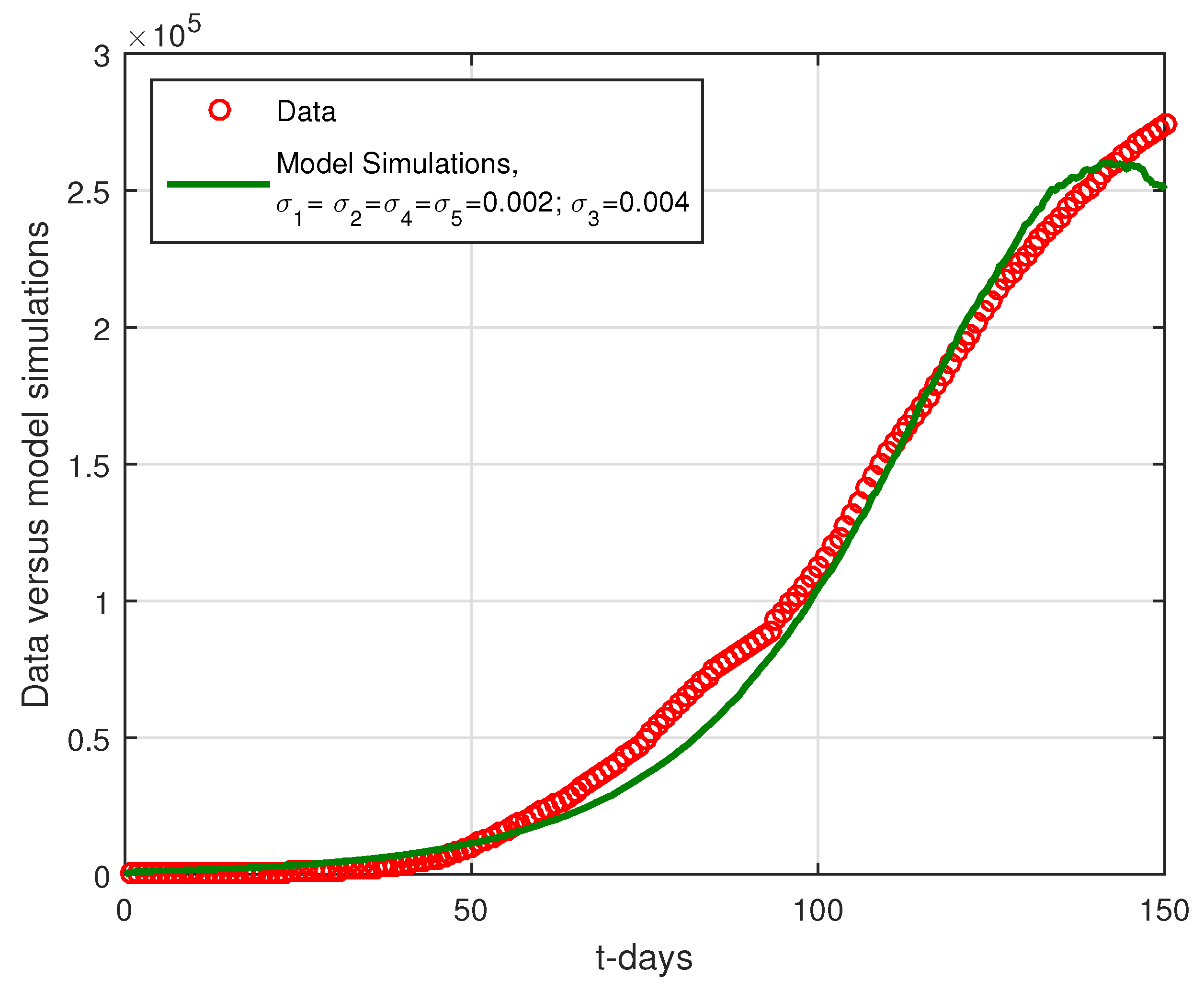
This section studies the estimation of the parameters for the model using the nonlinear least square curve fitting method. The data is considered for the infected cases of COVID-19 in Saudi Arabia. The cases are available in worldometers [37]. We consider the cases per day, thus, we consider the time unit given by per-day. Among these model parameters, we consider the demographic parameters of birth and the natural death rate that are obtained using estimations while the rest of the parameter values have been obtained through model fitting to the data. The stochastic model (3) is used to obtain the parameter estimations. We consider the infected cases of the Kingdom of Saudi Arabia of coronavirus infection for the period starting March–July 2020 [38] is considered. The total population is considered to be N ( 0 ) = 34 , 813 , 871 in Saudi Arabia in 2020 [39]. The average lifespan in the Kingdom of Saudi Arabia is given by 1 / 74.87 [40]. The birth rate is determined from the equation λ = d N ( 0 ) which is Λ = 1273.94 per day. The initial conditions are S ( 0 ) = 34 , 811 , 870 , E ( 0 ) = 2000 , I ( 0 ) = 1 , A ( 0 ) = R ( 0 ) = 0 . The basic reproduction number obtained through the data fitting is approximate R 0 = 1.1367 . The graphics for the data fitting are given in Figure 1 and Figure 2, while the parameters definitions and their realistic values are given in Table 1. Moreover, in Figure 1 and Figure 2, the legend “Data” referred to the infected cases while the “Model simulation” is the solution of the model”. Figure 1 is the model versus data fitting in the absence of σ i = 0 , for i = 1 , 2 , , 5 while Figure 2 is the data fitting versus model using σ 1 = σ 2 = σ 4 = σ 5 = 0.002 and σ 5 = 0.004 . Figure 3 describes the comparison of stochastic and deterministic models versus infected data. It is clear that the stochastic case provides good results for data compared to the deterministic case. It should be noted that in Figure 1 and Figure 2, the legend “Data” referred to the infected cases while the “Model simulation” is the solution of the model. The fitting with the stochastic case is better than the deterministic case.

6. Numerical Results

This section is divided into three subsections where we study the numerical scheme, the results, and finally in the last subsection, the discussion on the results achieved for Model (3). We first present a numerical algorithm for solving the model, then obtain graphical results with a detailed discussion.

6.1. Numerical Scheme

We give the following numerical scheme for the model (3) using the scheme adopted from [41] called the Milstein method to obtain the numerical results. It follows from [41] by writing our model (3) in the following form:
S i + 1 = S i + Λ β 1 E i + β 2 I i + β 3 A i S i N d S i t + σ 1 S i t ς 1 , i + σ 1 2 2 S i ( ς 1 , i 2 1 ) t , E i + 1 = E i + β 1 E i + β 2 I i + β 3 A i S i N ( δ + d ) E i t + σ 2 E i t ς 2 , i + σ 2 2 2 E i ( ς 2 , i 2 1 ) t , I i + 1 = I i + ( 1 τ ) δ E i d + d 1 + γ 1 I i t + ξ 3 I i t ς 3 , i + σ 3 2 2 I i ( ς 3 , i 2 1 ) t , A i + 1 = A i + τ δ E i d + γ 2 A i t + σ 4 A i t ς 4 , i + σ 4 2 2 A i ( ς 4 , i 2 1 ) t , R i + 1 = R i + γ 1 I i + γ 2 A i d R i t + σ 5 R i t ς 5 , i + σ 5 2 2 R i ( ς 5 , i 2 1 ) t .
In the above scheme, ς i , j , when i = 1 , , 5 , displays the independent Gaussian random variables with the given distribution N ( 0 , 1 ) , and where the step size is shown by Δ t , and σ i > 0 , for i = 1 , , 5 represents the numerical values of the noise.

6.2. Results

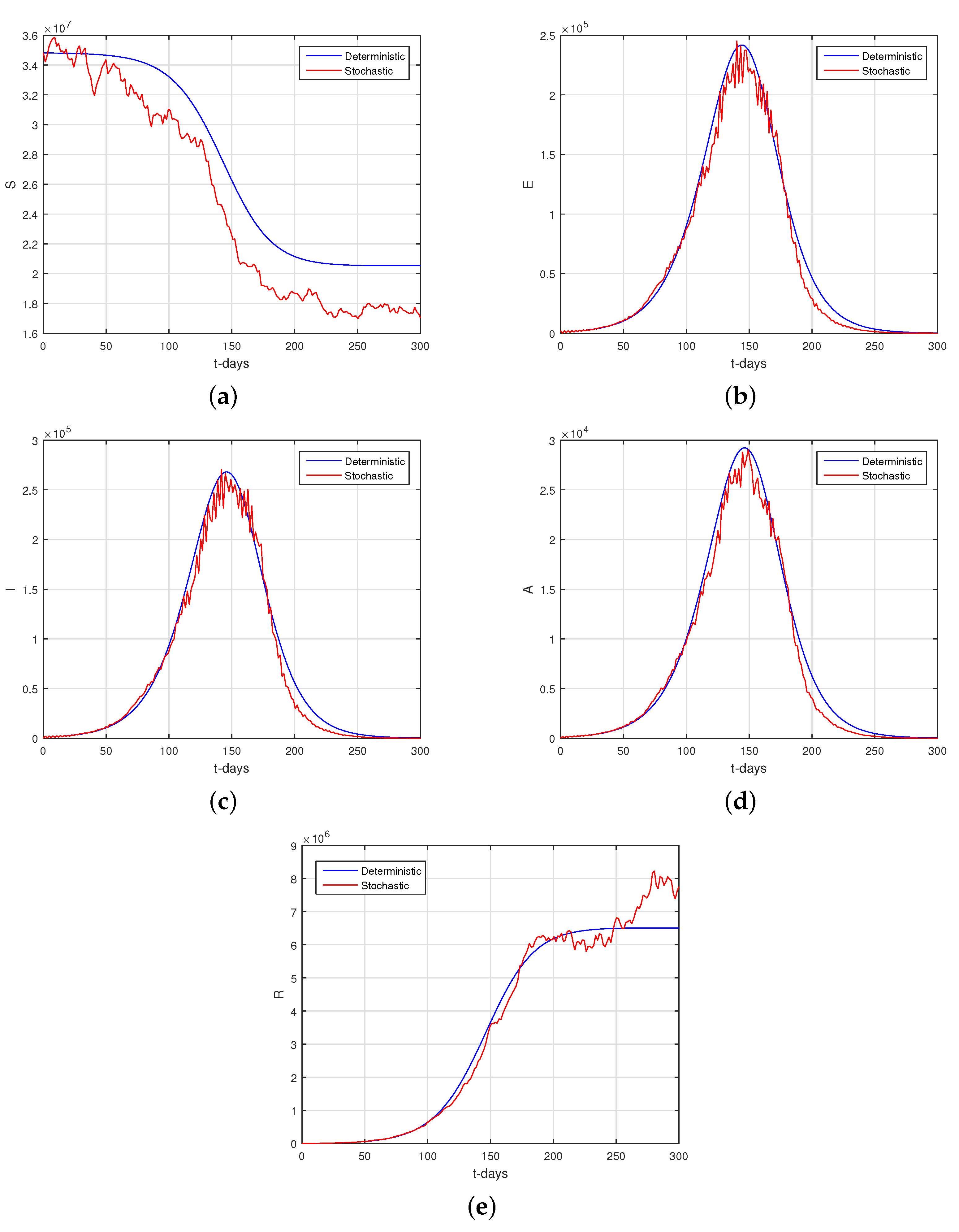
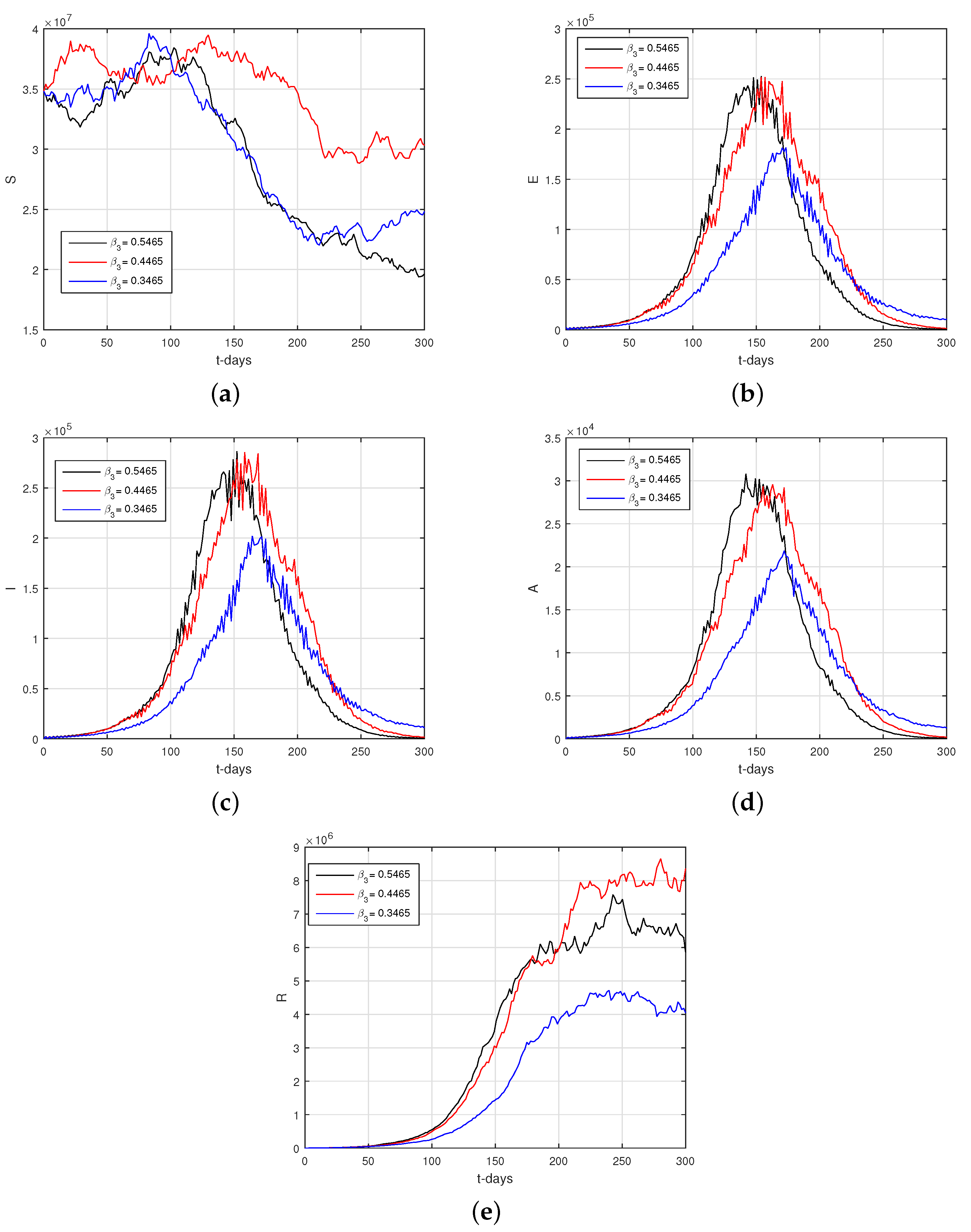
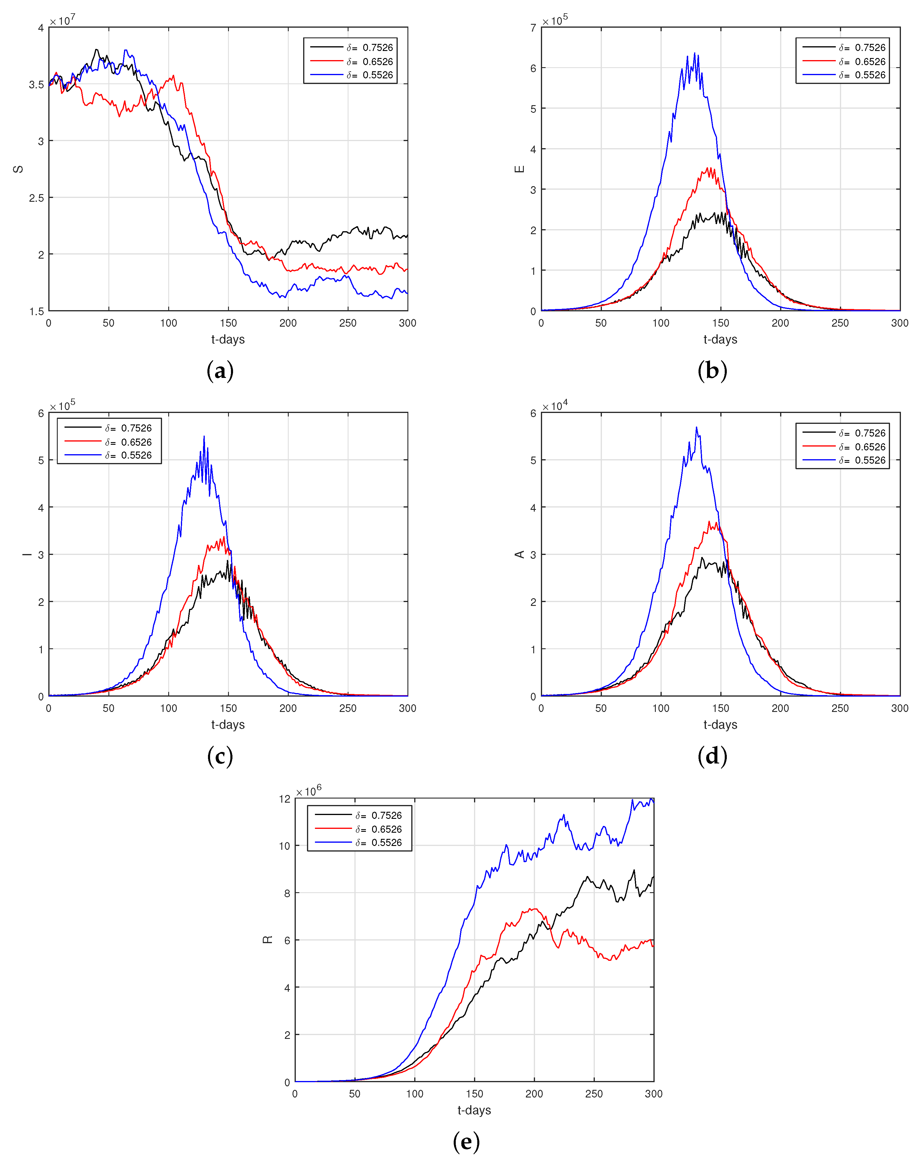
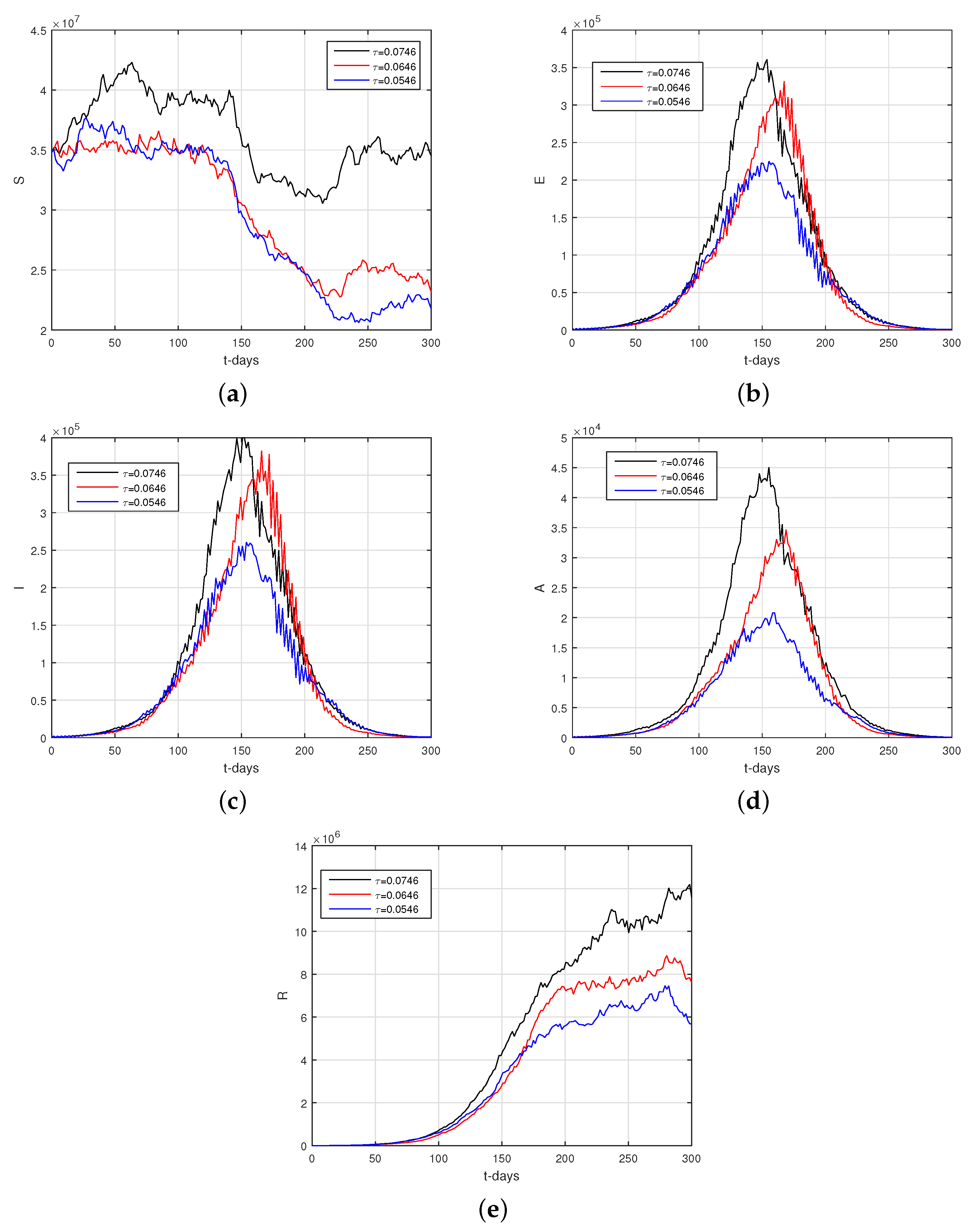
We solve the stochastic model (3) using the values of the parameters given in Table 1 and obtain the required graphical results, see Figure 4, Figure 5, Figure 6, Figure 7, Figure 8 and Figure 9. We use in these graphical results the values of the stochastic noises are σ 1 = 0.01 , σ 2 = 0.02 , σ 3 = 0.04 , σ 4 = 0.02 , σ 5 = 0.02 . The subgraphs in Figure 4, Figure 5, Figure 6, Figure 7, Figure 8 and Figure 9 represent the population of susceptible, exposed, infected with disease symptoms, infected with no disease symptoms, and the recovery individuals, respectively, in (a–e). Figure 4 represents the simulation of the stochastic model versus the deterministic model.
Figure 5 represents the simulation of the model for different values of β 1 . Reducing the contact between exposed and susceptible decreases the number of infective cases, also, one can see a better reduction in future cases if we restrict healthy individuals by following WHO recommendations.
Figure 6 gives the simulation of the stochastic model for many values of the parameter β 2 . We can obtain a better decrease if the contact among healthy and symptomatic individuals is decreased, so β 2 can decrease best the number of infected cases caused by the symptomatic infected individuals.
Similarly, we can see from Figure 7 the decrease in the parameter β 3 decreases the number of infected people due to the asymptomatic infection.
The impact of the parameters δ and τ is shown in Figure 8 and Figure 9.

6.3. Discussion

The graphical results obtained in this paper can be helpful regarding disease elimination in the country. The comparison of the stochastic and the deterministic model is shown in Figure 4. In particular, in Figure 4e, it can be seen that the number of recovered cases increases in the stochastic case as compared to the deterministic case. Increasing the testing of people and identifications of the symptomatic and asymptomatic individuals by quarantine and educating them about the disease can best minimize the future infected cases in the population. It is useful if individuals in a certain country increase COVID-19 testing upon identifying the asymptomatic and symptomatic individuals. The asymptomatic individuals that do not show visible disease symptoms should be isolated in order to decrease the future risk of infected cases. The symptomatic individuals should be quarantined, possibly at home, and can also be restricted from visiting other places which can possibly increase the population of infected cases in society. It can be seen from the graphical results that the model behaves well and leads to the equilibrium point.

7. Conclusions

In this work, we presented the analysis of the COVID-19 model using stochastic differential equations. We first formulated the model in ordinary differential equations and then we extended it to stochastic differential equations. We studied with care the stochastic COVID-19 mathematical model and presented their mathematical as well as numerical results in detail. Initially, we formulated the model by taking into account the assumptions of the transmission coefficients, such as exposed, symptomatic, and asymptomatic with their interaction with healthy people. It is well-known that these interactions are possible methods of increasing the cases of COVID-19 in a population. With these assumptions, we extended the model into stochastic differential equations. We studied the analysis of the model for the deterministic case and presented the related mathematical results for it. We proved the existence and uniqueness of the deterministic model and found the existence and uniqueness of the model. We studied the existence of the endemic equilibria and found that the model has a unique endemic equilibrium. We found that the deterministic model is globally asymptotically stable when the basic reproduction number R 0 1 .
Further, we studied the stochastic model and presented their unique global positive solution. We carried out the results of extinction for the stochastic model. The extinction results for the stochastic model have been provided.
We used the infected cases of the Kingdom of Saudi Arabia for the period March–July 2020 and parameterized the model. Using the nonlinear square curve fitting method, we obtained the data fitting to the model and presented it graphically. The results of the stochastic case for different σ i values have good fitting as compared to the deterministic case.
The obtained parameters from the least square curve fit have been used to obtain the numerical results. The basic reproduction number computed for the given set of parameters is approximately, R 0 1.1367 .
We also compared the data fitting to the model using deterministic and stochastic and showed that stochastic fitting is better than the deterministic case for this work, and present a comparative graph of both solutions. We gave a comparison of graphical results for the case of deterministic and stochastic solutions. Some important parameters that can possibly best decrease future cases have been shown graphically. Among these parameters, the contact between susceptible and exposed, susceptible and symptomatic, and susceptible and asymptomatic, can best decrease future cases, if the recommendations of the World Health Organization (WHO) are properly followed.
According to the results of our simulations, one can see that our results are in line with the WHO recommendations and can be useful for disease elimination in the country of Saudi Arabia, see for more details [42,43].

Author Contributions

Conceptualization, M.A.K., A.D. and P.S.; Data curation, F.S.A., F.T.A. and A.D.; Formal analysis, F.T.A., M.A.K. and P.S.; Investigation, F.S.A., M.A.K., A.D. and P.S.; Methodology, F.S.A., F.T.A., M.A.K. and A.D.; Project administration, F.S.A., F.T.A. and P.S.; Resources, F.S.A. and M.A.K.; Software, F.T.A. and P.S.; Supervision, M.A.K. and P.S.; Visualization, F.S.A., F.T.A. and M.A.K.; Writing—original draft, F.S.A., F.T.A., M.A.K., A.D. and P.S. All authors have read and agreed to the published version of the manuscript.

Funding

The APC of this paper was funded by the Deanship of Scientific Research at Imam Mohammad Ibn Saud Islamic University.

Data Availability Statement

Data is available from the corresponding author on a reasonable request.

Acknowledgments

The authors extend their appreciation to the Deanship of Scientific Research at Imam Mohammad Ibn Saud Islamic University for funding this work through Research Group no. RG-21-09-16.

Conflicts of Interest

The authors declare no conflict of interest.

References

  1. Khan, M.A.; Atangana, A. Modeling the dynamics of novel coronavirus (2019-nCov) with fractional derivative. Alex. Eng. J. 2020, 59, 2379–2389. [Google Scholar] [CrossRef]
  2. Khan, M.A.; Atangana, A.; Alzahrani, E.; Fatmawati. The dynamics of COVID-19 with quarantined and isolation. Adv. Differ. Equ. 2020, 2020, 425. [Google Scholar] [CrossRef]
  3. Oud, M.A.A.; Ali, A.; Alrabaiah, H.; Ullah, S.; Khan, M.A.; Islam, S. A fractional order mathematical model for COVID-19 dynamics with quarantine, isolation, and environmental viral load. Adv. Differ. Equ. 2021, 2021, 106. [Google Scholar] [CrossRef]
  4. Rihan, F.; Alsakaji, H. Dynamics of a stochastic delay differential model for COVID-19 infection with asymptomatic infected and interacting people: Case study in the UAE. Results Phys. 2021, 28, 104658. [Google Scholar] [CrossRef] [PubMed]
  5. Anggriani, N.; Ndii, M.Z.; Amelia, R.; Suryaningrat, W.; Pratama, M.A.A. A mathematical COVID-19 model considering asymptomatic and symptomatic classes with waning immunity. Alex. Eng. J. 2022, 61, 113–124. [Google Scholar] [CrossRef]
  6. Masandawa, L.; Mirau, S.S.; Mbalawata, I.S. Mathematical modeling of COVID-19 transmission dynamics between healthcare workers and community. Results Phys. 2021, 29, 104731. [Google Scholar] [CrossRef] [PubMed]
  7. Rwezaura, H.; Tchoumi, S.; Tchuenche, J. Impact of environmental transmission and contact rates on Covid-19 dynamics: A simulation study. Informatics Med. Unlocked 2021, 27, 100807. [Google Scholar] [CrossRef]
  8. Liu, X.; Ullah, S.; Alshehri, A.; Altanji, M. Mathematical assessment of the dynamics of novel coronavirus infection with treatment: A fractional study. Chaos Solitons Fractals 2021, 153, 111534. [Google Scholar] [CrossRef]
  9. Beigi, A.; Yousefpour, A.; Yasami, A.; Gómez-Aguilar, J.; Bekiros, S.; Jahanshahi, H. Application of reinforcement learning for effective vaccination strategies of coronavirus disease 2019 (COVID-19). Eur. Phys. J. Plus 2021, 136, 609. [Google Scholar] [CrossRef] [PubMed]
  10. Martinez-Guerra, R.; Flores-Flores, J.P. An algorithm for the robust estimation of the COVID-19 pandemics population by considering undetected individuals. Appl. Math. Comput. 2021, 405, 126273. [Google Scholar] [PubMed]
  11. Riyapan, P.; Shuaib, S.E.; Intarasit, A. A Mathematical model of COVID-19 Pandemic: A case study of Bangkok, Thailand. Comput. Math. Methods Med. 2021, 2021, 6664483. [Google Scholar] [CrossRef] [PubMed]
  12. Khan, M.A.; Ullah, S.; Kumar, S. A robust study on 2019-nCOV outbreaks through non-singular derivative. Eur. Phys. J. Plus 2021, 136, 168. [Google Scholar] [CrossRef]
  13. Bock, W.; Jayathunga, Y.; Götz, T.; Rockenfeller, R. Are the upper bounds for new SARS-CoV-2 infections in Germany useful? Comput. Math. Biophys. 2021, 9, 242–260. [Google Scholar] [CrossRef]
  14. Khan, M.A.; Atangana, A. Mathematical modeling and analysis of COVID-19: A study of new variant Omicron. Phys. A Stat. Mech. Its Appl. 2022, 599, 127452. [Google Scholar] [CrossRef] [PubMed]
  15. Muniyappan, A.; Sundarappan, B.; Manoharan, P.; Hamdi, M.; Raahemifar, K.; Bourouis, S.; Varadarajan, V. Stability and numerical solutions of second wave mathematical modeling on covid-19 and omicron outbreak strategy of pandemic: Analytical and error analysis of approximate series solutions by using hpm. Mathematics 2022, 10, 343. [Google Scholar] [CrossRef]
  16. Pandey, P.; Gómez-Aguilar, J.; Kaabar, M.K.; Siri, Z.; Abd Allah, A.M. Mathematical modeling of COVID-19 pandemic in India using Caputo-Fabrizio fractional derivative. Comput. Biol. Med. 2022, 145, 105518. [Google Scholar] [CrossRef] [PubMed]
  17. Asamoah, J.K.K.; Okyere, E.; Abidemi, A.; Moore, S.E.; Sun, G.Q.; Jin, Z.; Acheampong, E.; Gordon, J.F. Optimal control and comprehensive cost-effectiveness analysis for COVID-19. Results Phys. 2022, 33, 105177. [Google Scholar] [CrossRef]
  18. Khajanchi, S.; Sarkar, K.; Banerjee, S. Modeling the dynamics of COVID-19 pandemic with implementation of intervention strategies. Eur. Phys. J. Plus 2022, 137, 129. [Google Scholar] [CrossRef]
  19. Ullah, M.S.; Higazy, M.; Kabir, K.A. Modeling the epidemic control measures in overcoming COVID-19 outbreaks: A fractional-order derivative approach. Chaos Solitons Fractals 2022, 155, 111636. [Google Scholar] [CrossRef] [PubMed]
  20. Tesfaye, A.W.; Satana, T.S. Stochastic model of the transmission dynamics of COVID-19 pandemic. Adv. Differ. Equ. 2021, 2021, 457. [Google Scholar] [CrossRef] [PubMed]
  21. Rihan, F.A.; Alsakaji, H.J.; Rajivganthi, C. Stochastic SIRC epidemic model with time-delay for COVID-19. Adv. Differ. Equ. 2020, 2020, 502. [Google Scholar] [CrossRef] [PubMed]
  22. Niño-Torres, D.; Ríos-Gutiérrez, A.; Arunachalam, V.; Ohajunwa, C.; Seshaiyer, P. Stochastic modeling, analysis, and simulation of the COVID-19 pandemic with explicit behavioral changes in Bogotá: A case study. Infect. Dis. Model. 2022, 7, 199–211. [Google Scholar] [CrossRef] [PubMed]
  23. Tesfay, A.; Saeed, T.; Zeb, A.; Tesfay, D.; Khalaf, A.; Brannan, J. Dynamics of a stochastic COVID-19 epidemic model with jump-diffusion. Adv. Differ. Equ. 2021, 2021, 228. [Google Scholar] [CrossRef] [PubMed]
  24. Guo, X.; Gupta, A.; Sampat, A.; Zhai, C. A stochastic contact network model for assessing outbreak risk of COVID-19 in workplaces. PLoS ONE 2022, 17, e0262316. [Google Scholar] [CrossRef] [PubMed]
  25. Allen, L.J. A primer on stochastic epidemic models: Formulation, numerical simulation, and analysis. Infect. Dis. Model. 2017, 2, 128–142. [Google Scholar] [CrossRef] [PubMed]
  26. Zhong, H.; Wang, W. Mathematical analysis for COVID-19 resurgence in the contaminated environment. Math. Biosci. Eng. 2020, 17, 6909–6927. [Google Scholar] [CrossRef]
  27. Li, S.; Ying, S. Latest Research Advances on Novel Coronavirus Pneumonia. 2020, SciFinder; 2020. Preprint|SciFinder|ID: Ppcovidwho-4385. Available online: https://pesquisa.bvsalud.org/global-literature-on-novel-coronavirus-2019-ncov/resource/pt/ppcovidwho-4385 (accessed on 20 September 2022).
  28. Chen, Y.; Wang, A.; Yi, B.; Ding, K.; Wang, H.; Wang, J.; Shi, H.; Wang, S.; Xu, G. Epidemiological characteristics of infection in COVID-19 close contacts in Ningbo city. Zhonghua Liu Xing Bing Xue Zhi Zhonghua Liuxingbingxue Zazhi 2020, 41, 667–671. [Google Scholar]
  29. Heilongjiang Provincial Health Committee. Available online: http://wsjkw.hlj.gov.cn/ (accessed on 10 July 2022).
  30. Xiong, C. A detailed explanation of survival time for COVID-19 virus in the environment. China Food Safty Mag. 2020, 5, 22–25. [Google Scholar]
  31. Van den Driessche, P.; Watmough, J. Reproduction numbers and sub-threshold endemic equilibria for compartmental models of disease transmission. Math. Biosci. 2002, 180, 29–48. [Google Scholar] [CrossRef]
  32. Mao, X. Stochastic Differential Equations and their Applications; Horwood Publ.: Chichester, UK, 1997. [Google Scholar]
  33. Zhang, Q.; Zhou, K. Stationary distribution and extinction of a stochastic SIQR model with saturated incidence rate. Math. Probl. Eng. 2019, 2019, 3575410. [Google Scholar] [CrossRef]
  34. Din, A.; Liang, J.; Zhou, T. Detecting critical transitions in the case of moderate or strong noise by binomial moments. Phys. Rev. E 2018, 98, 012114. [Google Scholar] [CrossRef] [PubMed]
  35. Zhao, Y.; Jiang, D. The threshold of a stochastic SIRS epidemic model with saturated incidence. Appl. Math. Lett. 2014, 34, 90–93. [Google Scholar] [CrossRef]
  36. Zhao, Y.; Jiang, D. The threshold of a stochastic SIS epidemic model with vaccination. Appl. Math. Comput. 2014, 243, 718–727. [Google Scholar] [CrossRef]
  37. World/Countries/Saudi Arabia. Available online: https://www.worldometers.info/coronavirus/country/saudi-arabia/ (accessed on 20 September 2022).
  38. Daily New Cases in Saudi Arabia. Available online: https://www.worldometers.info/coronavirus/country/saudi-arabia/ (accessed on 20 September 2022).
  39. Saudi Arabia Population. Available online: https://www.worldometers.info/world-population/saudi-arabia-population/ (accessed on 20 September 2022).
  40. Life Expectancy at Birth, Total (Years)—Saudi Arabia. Available online: https://data.worldbank.org/indicator/SP.DYN.LE00.IN?locations=SA (accessed on 20 September 2022).
  41. Higham, D.J. An algorithmic introduction to numerical simulation of stochastic differential equations. SIAM Rev. 2001, 43, 525–546. [Google Scholar] [CrossRef]
  42. Yezli, S.; Khan, A. COVID-19 social distancing in the Kingdom of Saudi Arabia: Bold measures in the face of political, economic, social and religious challenges. Travel Med. Infect. Dis. 2020, 37, 101692. [Google Scholar] [CrossRef] [PubMed]
  43. Al-Harbi, S.K.; Al-Tuwairqi, S.M. Modeling the effect of lockdown and social distancing on the spread of COVID-19 in Saudi Arabia. PLoS ONE 2022, 17, e0265779. [Google Scholar] [CrossRef] [PubMed]
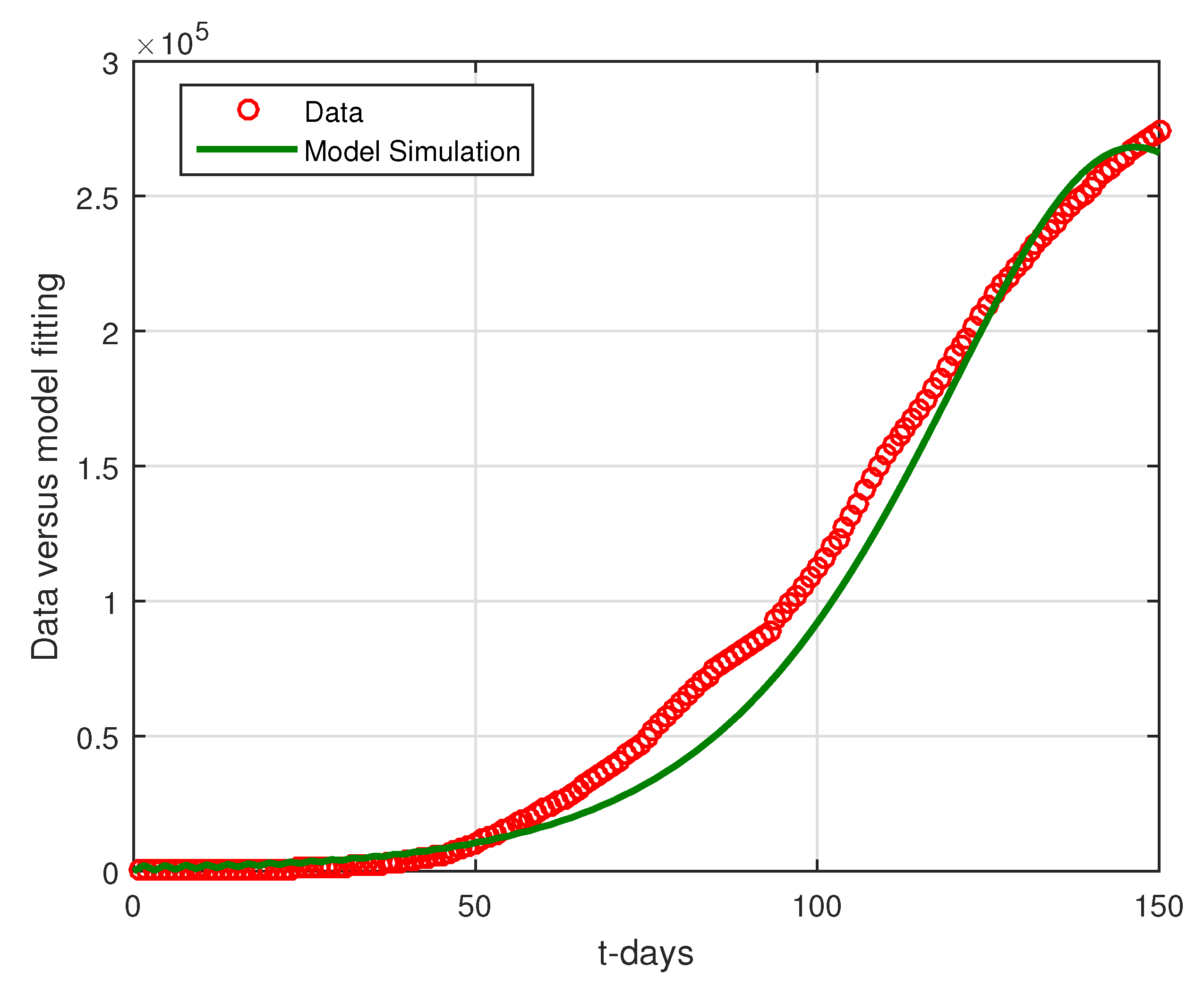
Figure 1. Model fitting with deterministic cases when R 0 = 1.1367 > 1 . The circle denotes the infected cases while the bold line referred to the model solutions.
Symmetry 14 02521 g001
Figure 2. Model fitting for the stochastic case. The circle denotes the infected cases while the bold line referred to the model solutions.
Symmetry 14 02521 g002
Figure 3. Data fitting using stochastic and deterministic models, blue line “stochastic case”, red line “deterministic case” while the circle shows infected cases.
Symmetry 14 02521 g003
Figure 4. The comparison of stochastic and deterministic model. For the stochastic model, we consider the values σ 1 = 0.01 , σ 3 = 0.04 , σ 2 = σ 4 = σ 5 = 0.02 . Subfigures (ae) represent, respectively, the comparison of healthy, exposed, symptomatic infected, asymptomatic infected and the recovered with and without stochastic noise.
Symmetry 14 02521 g004
Figure 5. The impact of the parameter β 1 on the stochastic model. Subfigures (ae) represent, respectively, the dynamics of susceptible, exposed, symptomatic, asymptomatic and recovered population under different values of the parameters β 1 .
Symmetry 14 02521 g005
Figure 6. The impact of the parameter β 2 on the stochastic model. Subfigures (ae) represent, respectively, the dynamics of susceptible, exposed, symptomatic, asymptomatic and recovered population under different values of the parameters β 2 .
Symmetry 14 02521 g006
Figure 7. The impact of the parameter β 3 on the stochastic model. Subfigures (ae) represent, respectively, the dynamics of susceptible, exposed, symptomatic, asymptomatic and recovered population under different values of the parameters β 3 .
Symmetry 14 02521 g007
Figure 8. The plot shows the simulation with δ for the stochastic model. Subfigures (ae) represent, respectively, the dynamics of susceptible, exposed, symptomatic, asymptomatic and recovered population under different values of the parameters δ .
Symmetry 14 02521 g008
Figure 9. The impact of the parameter τ on the stochastic model. Subfigures (ae) represent, respectively, the dynamics of susceptible, exposed, symptomatic, asymptomatic and recovered population under different values of the parameters τ .
Symmetry 14 02521 g009
Table 1. Parameters used in data fitting.
ParameterDescriptionValueSource
Λ Birth rate1273.94Estimated
dNatural death rate 1 74.87 × 365 Estimated
β 1 Contact rate among E and S0.1321Fitted
β 2 Contact rate among I and S0.5926Fitted
β 3 Contact rate among A and S0.5465Fitted
δ Incubation period0.7526Fitted
τ Incubation period0.0746Fitted
d 1 Natural mortality due to disease0.3691Fitted
γ 1 Recovery from I0.2588Fitted
γ 2 Recovery from A0.4639Fitted
Publisher’s Note: MDPI stays neutral with regard to jurisdictional claims in published maps and institutional affiliations.