
Estimating the Spread of Generalized Compartmental Model of Monkeypox Virus Using a Fuzzy Fractional Laplace Transform Method
 , , , and
Abstract
:1. Introduction
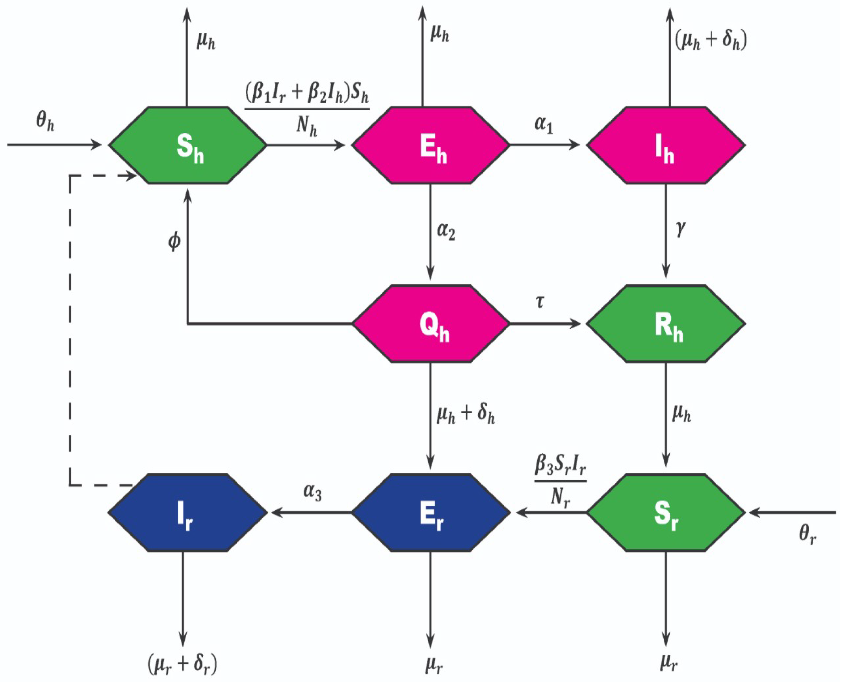
2. Mathematical Modelling
3. Fuzzy Fractional Analysis in the Monkeypox Model
3.1. A Fuzzy Fractional Model’S Existence Furthermore, Uniqueness
- The mathematical model’s beginning conditions should have a solution.
- We want every mathematical model to have a single solution that is determined by the initial conditions. Now, rewriting Equation (3) in the form ofwhere the fuzzy functions are . Therefore,which subject to the initial conditions
3.2. Scheme of the Solution
- (i)
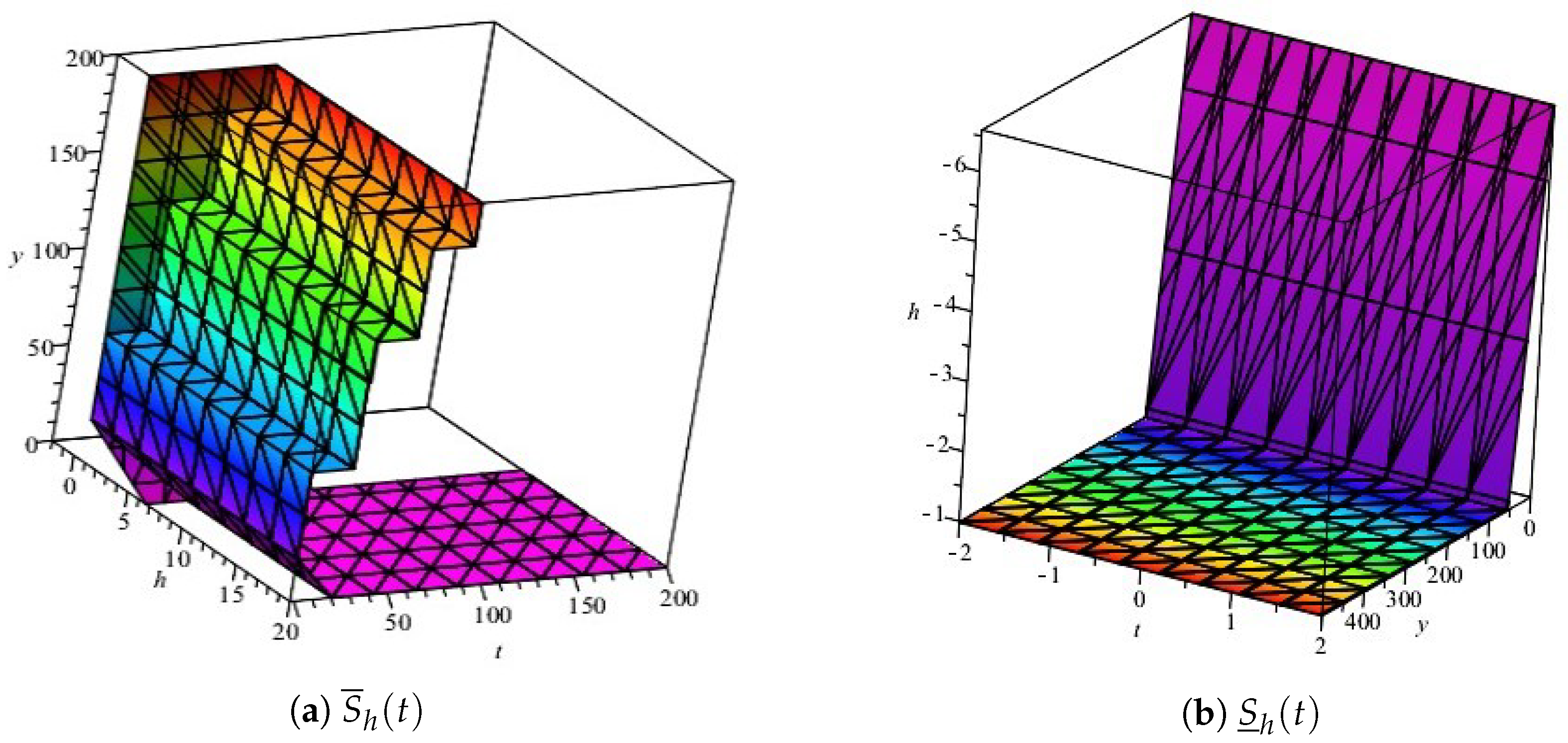
- Human suspected case:
- (ii)
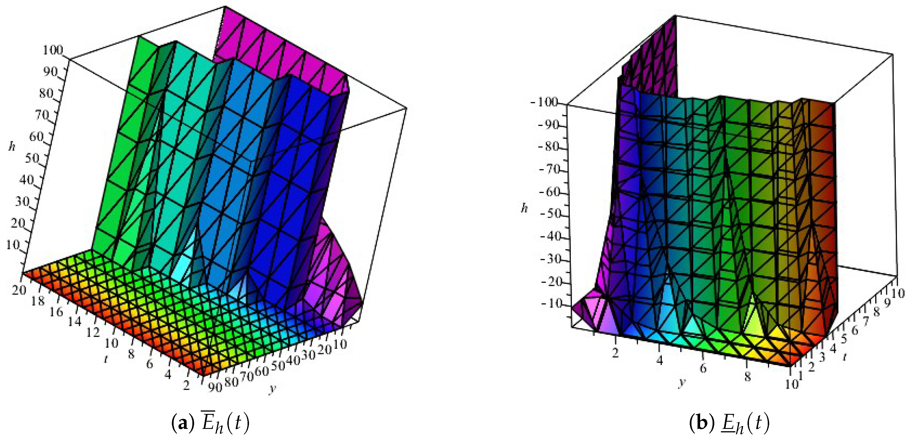
- Human-exposed case:
- (iii)
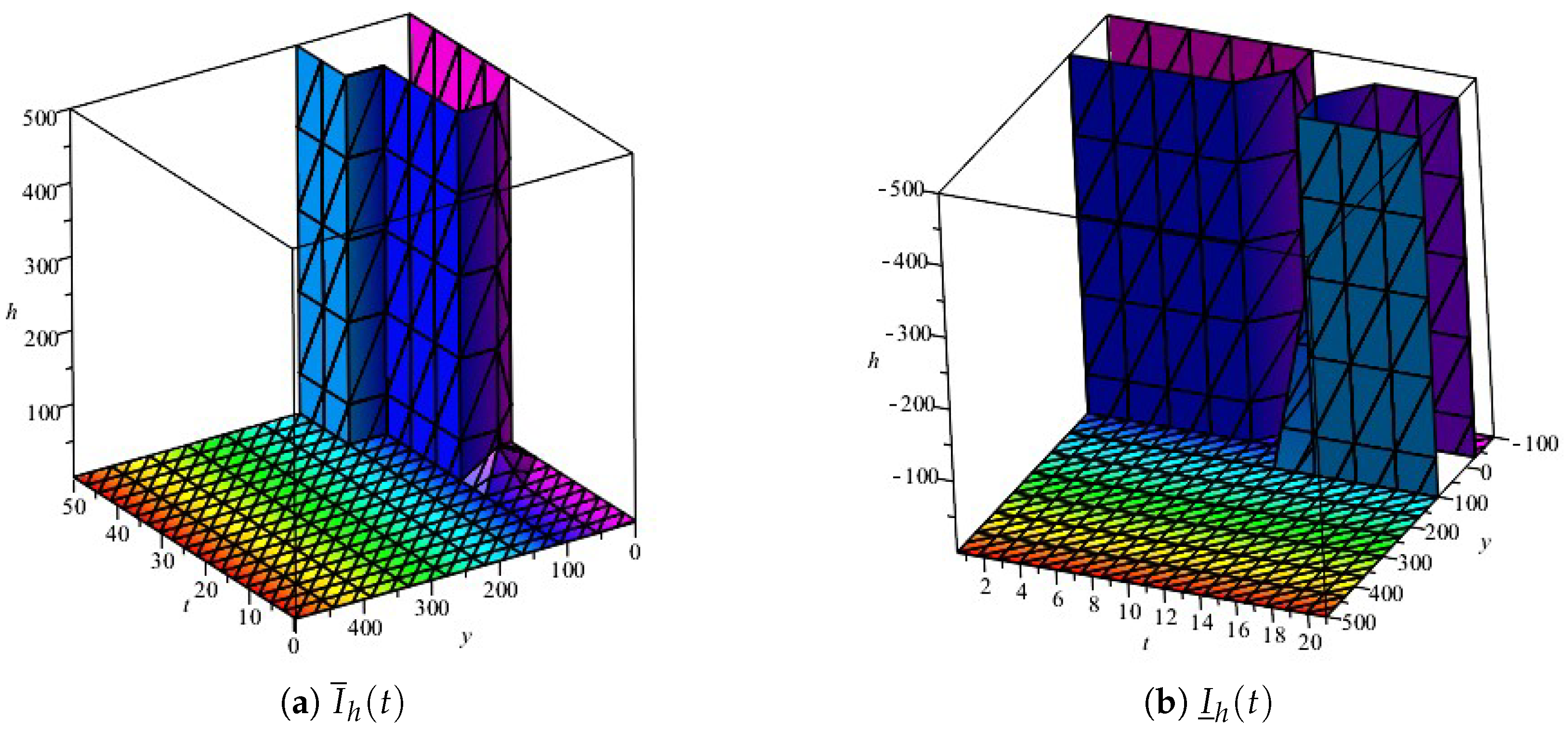
- Human-infected case:
- (iv)
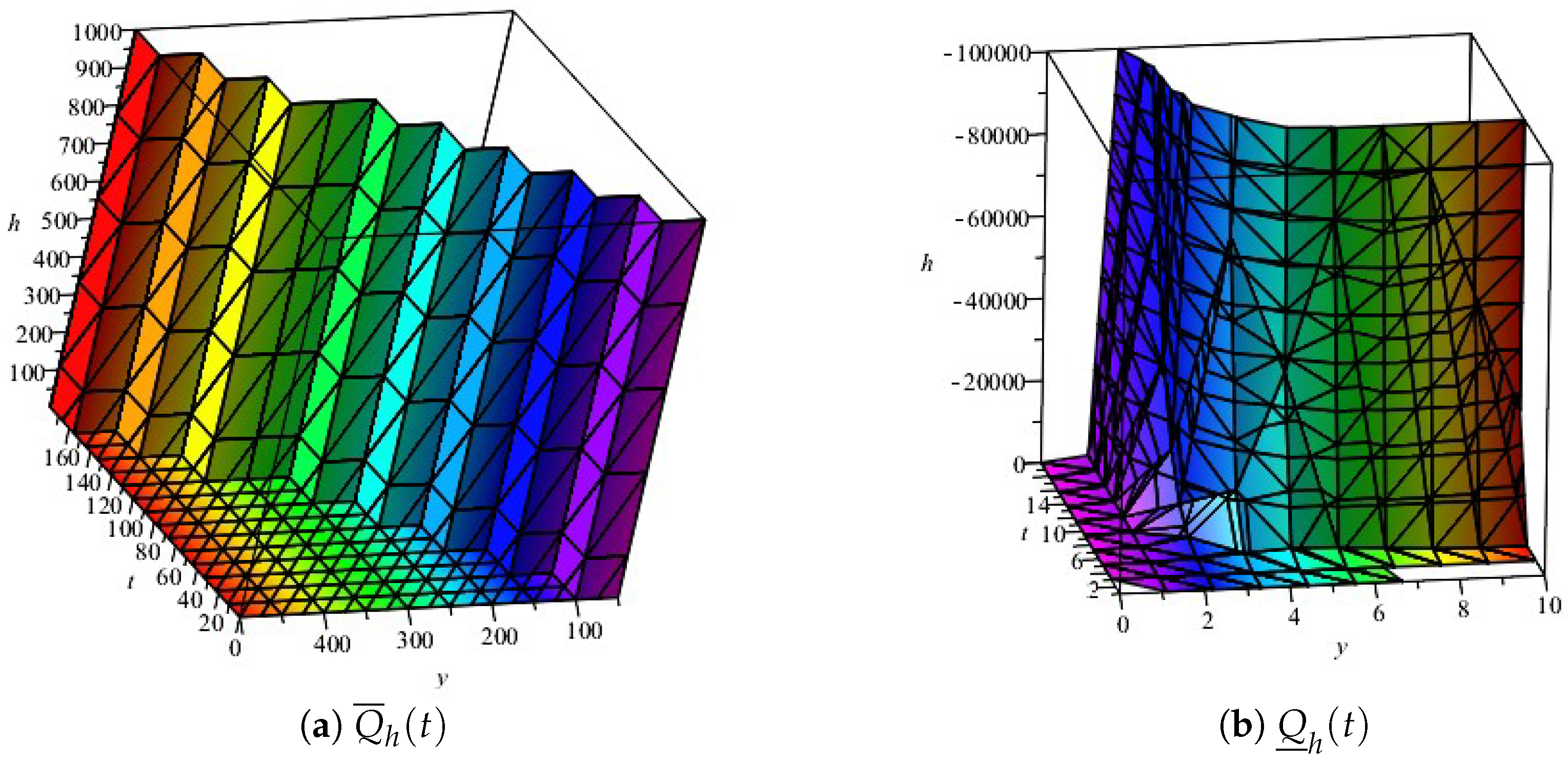
- Human-quarantined case:
- (v)
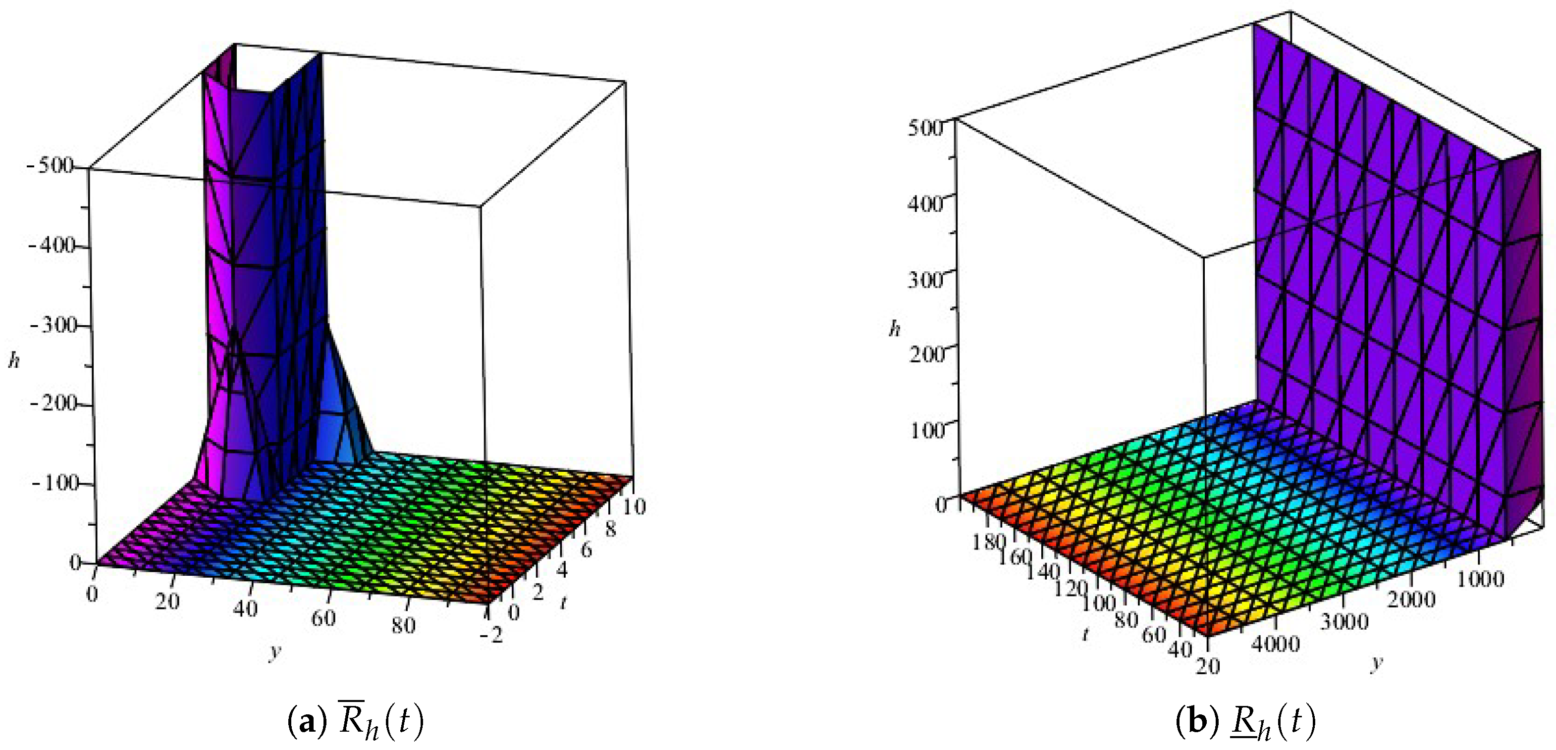
- Human recovered case:
- (vi)
- Rodent suspected case:
- (vii)
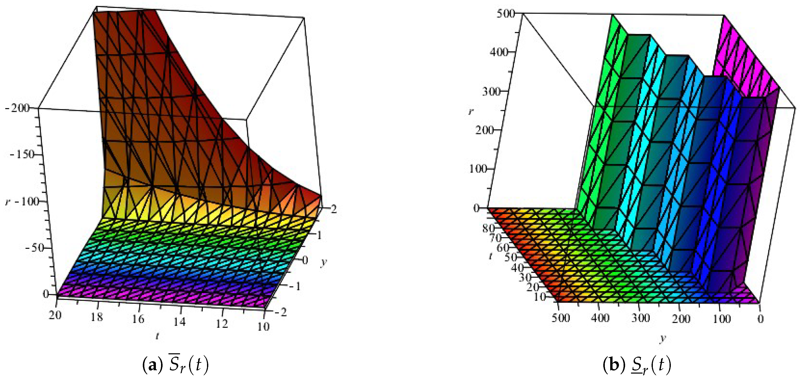
- Rodent exposed case:
- (viii)
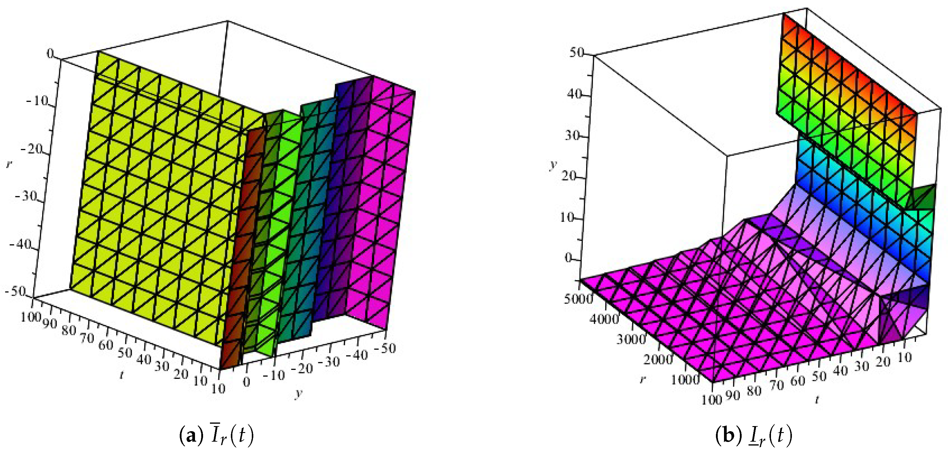
- Rodent-infected case:
4. Results Furthermore, Discussion
Generalized Compartmental Model
5. Conclusions
Author Contributions
Funding
Institutional Review Board Statement
Informed Consent Statement
Data Availability Statement
Acknowledgments
Conflicts of Interest
References
- World Health Organization. Monkeypox. 2022. Available online: https://www.who.int/news-room/fact-sheets/detail/monkeypox (accessed on 19 May 2022).
- McCollum, A.M.; Damon, I.K. Human monkeypox. Clin. Infect. Dis. 2014, 58, 260–267. [Google Scholar] [CrossRef] [PubMed] [Green Version]
- Fine, P.E.; Jezek, Z.; Grab, B.; Dixon, H. The transmission potential of monkeypox virus in human populations. Int. J. Epidemiol. 1988, 17, 643–650. [Google Scholar] [CrossRef] [PubMed]
- Nolen, L.D.; Osadebe, L.; Katomba, J.; Likofata, J.; Mukadi, D.; Monroe, B.; Doty, J.; Hughes, C.M.; Kabamba, J.; Malekani, J.; et al. Extended human-to-human transmission during a monkeypox outbreak in the Democratic Republic of the Congo. Emerg. Infect. Dis. 2016, 22, 1014. [Google Scholar] [CrossRef] [PubMed] [Green Version]
- Kavanagh, K. Monkeypox: CDC Raises Travel Alert, However, How Much Threat Is It Really? 2022. Available online: https://www.infectioncontroltoday.com/view/monkeypox-cdc\-raises-travel-alert-but-how-much-threat-is-it-really (accessed on 18 July 2022).
- Mahase, E. Monkeypox: Healthcare workers will be offered smallpox vaccine as UK buys 20,000 doses. BMJ 2022, 377, o1379. [Google Scholar] [CrossRef] [PubMed]
- Strassburg, M.A. The global eradication of smallpox. Am. J. Infect. Control 1982, 10, 53–59. [Google Scholar] [CrossRef] [PubMed]
- Moss, B. Genetically engineered poxviruses for recombinant gene expression, vaccination, and safety. Proc. Natl. Acad. Sci. USA 1996, 93, 11341–11348. [Google Scholar] [CrossRef] [Green Version]
- Henderson, D.A. Smallpox: Clinical and Epidemiologic Features. Emerg. Infect. Dis. 1999, 5, 537–539. [Google Scholar] [CrossRef]
- Pennington, H. Smallpox and bioterrorism. Bull. World Health Organ. 2003, 81, 762–767. [Google Scholar]
- Silva, N.I.; de Oliveira, J.S.; Kroon, E.G.; Trindade, G.D.; Drumond, B.P. Here, there, and everywhere: The wide host range and geographic distribution of zoonotic orthopoxviruses. Viruses 2020, 13, 43. [Google Scholar] [CrossRef]
- Memariani, M.; Memariani, H. Multinational monkeypox outbreak: What do we know and what should we do? Ir. J. Med. Sci. 2022, 1–2. [Google Scholar] [CrossRef]
- Bunge, E.M.; Hoet, B.; Chen, L.; Lienert, F.; Weidenthaler, H.; Baer, L.R.; Steffen, R. The changing epidemiology of human monkeypox—A potential threat? A systematic review. PLoS Negl. Trop. Dis. 2022, 16, e0010141. [Google Scholar] [CrossRef] [PubMed]
- Vaughan, A.; Aarons, E.; Astbury, J.; Balasegaram, S.; Beadsworth, M.; Beck, C.R.; Chand, M.; Oconnor, C.; Dunning, J.; Ghebrehewet, S.; et al. Two cases of monkeypox imported to the United Kingdom, September 2018. Eurosurveillance 2018, 23, 1800509. [Google Scholar] [CrossRef] [PubMed] [Green Version]
- Reed, K.D.; Melski, J.W.; Graham, M.B.; Regnery, R.L.; Sotir, M.J.; Wegner, M.V.; Kazmierczak, J.J.; Stratman, E.J.; Li, Y.; Fairley, J.A.; et al. The detection of monkeypox in humans in the Western Hemisphere. N. Engl. J. Med. 2004, 350, 342–350. [Google Scholar] [CrossRef] [PubMed] [Green Version]
- Hutson, C.L.; Olson, V.A.; Carroll, D.S.; Abel, J.A.; Hughes, C.M.; Braden, Z.H.; Weiss, S.; Self, J.; Osorio, J.E.; Hudson, P.N.; et al. A prairie dog animal model of systemic orthopoxvirus disease using West African and Congo Basin strains of monkeypox virus. J. Gen. Virol. 2009, 90, 323–333. [Google Scholar] [CrossRef]
- Adler, H.; Gould, S.; Hine, P.; Snell, L.B.; Wong, W.; Houlihan, C.F.; Osborne, J.C.; Rampling, T.; Beadsworth, M.B.; Duncan, C.J.; et al. Clinical features and management of human monkeypox: A retrospective observational study in the UK. Lancet Infect. Dis. 2022, 22, 1153–1162. [Google Scholar] [CrossRef]
- Parker, S.; Buller, R.M. A review of experimental and natural infections of animals with monkeypox virus between 1958 and 2012. Future Virol. 2013, 8, 129–157. [Google Scholar] [CrossRef] [Green Version]
- Merchlinsky, M.; Albright, A.; Olson, V.; Schiltz, H.; Merkeley, T.; Hughes, C.; Petersen, B.; Challberg, M. The development and approval of tecoviromat (TPOXX®), the first antiviral against smallpox. Antivir. Res. 2019, 168, 168–174. [Google Scholar] [CrossRef]
- World Health Organization. Monkeypox. Available online: https://www.who.int/emergencies/emergency-events/item/monkeypox (accessed on 11 July 2022).
- WHO Director-General Declares the Ongoing Monkeypox Outbreak a Public Health Emergency of International Concern. Available online: https://www.who.int/europe/news/item/23-07-2022-who-director-general-declares-the-ongoing-monkeypox-outbreak-a-public-health-event-of-international-concern (accessed on 1 August 2022).
- Joint ECDC-WHO Regional Office for Europe Monkeypox Surveillance Bulletin. Available online: https://monkeypoxreport.ecdc.europa.eu/ (accessed on 9 August 2022).
- Barron, M. Monkeypox vs. COVID-19. American Society for Microbiology. 2022. Available online: https://asm.org/Articles/2022/August/Monkeypox-vs-COVID-19 (accessed on 19 August 2022).
- Almehmadi, M.; Allahyani, M.; Alsaiari, A.A.; Alshammari, M.K.; Alharbi, A.S.; Hussain, K.H.; Alsubaihi, L.I.; Kamal, M.; Alotaibi, S.S.; Alotaibi, A.N.; et al. A Glance at the Development and Patent Literature of Tecovirimat: The First-in-Class Therapy for Emerging Monkeypox Outbreak. Viruses 2022, 14, 1870. [Google Scholar] [CrossRef] [PubMed]
- Tiecco, G.; Degli Antoni, M.; Storti, S.; Tomasoni, L.R.; Castelli, F.; Quiros-Roldan, E. Monkeypox, a Literature Review: What Is New and Where Does This concerning Virus Come From? Viruses 2022, 14, 1894. [Google Scholar] [CrossRef]
- Ahmed, S.F.; Sohail, M.S.; Quadeer, A.A.; McKay, M.R. Vaccinia-Virus-Based Vaccines Are Expected to Elicit Highly Cross-Reactive Immunity to the 2022 Monkeypox Virus. Viruses 2022, 14, 1960. [Google Scholar] [CrossRef]
- Mucker, E.M.; Shamblin, J.D.; Goff, A.J.; Bell, T.M.; Reed, C.; Twenhafel, N.A.; Chapman, J.; Mattix, M.; Alves, D.; Garry, R.F.; et al. Evaluation of Virulence in Cynomolgus Macaques Using a Virus Preparation Enriched for the Extracellular Form of Monkeypox Virus. Viruses 2022, 14, 1993. [Google Scholar] [CrossRef] [PubMed]
- Mucker, E.M.; Shamblin, J.D.; Raymond, J.L.; Twenhafel, N.A.; Garry, R.F.; Hensley, L.E. Effect of Monkeypox Virus Preparation on the Lethality of the Intravenous Cynomolgus Macaque Model. Viruses 2022, 14, 1741. [Google Scholar] [CrossRef] [PubMed]
- Chmel, M.; Bartos, O.; Kabickova, H.; Pajer, P.; Kubickova, P.; Novotna, I.; Bartovska, Z.; Zlamal, M.; Burantova, A.; Holub, M.; et al. Retrospective Analysis Revealed an April Occurrence of Monkeypox in the Czech Republic. Viruses 2022, 14, 1773. [Google Scholar] [CrossRef] [PubMed]
- Israeli, O.; Guedj-Dana, Y.; Shifman, O.; Lazar, S.; Cohen-Gihon, I.; Amit, S.; Ben-Ami, R.; Paran, N.; Schuster, O.; Weiss, S.; et al. Rapid Amplicon Nanopore Sequencing (RANS) for the Differential Diagnosis of Monkeypox Virus and Other Vesicle-Forming Pathogens. Viruses 2022, 14, 1817. [Google Scholar] [CrossRef] [PubMed]
- Zafar, Z.U.; Shah, Z.; Ali, N.; Alzahrani, E.O.; Shutaywi, M. Mathematical and stability analysis of fractional order model for spread of pests in tea plants. Fractals 2021, 29, 2150008. [Google Scholar] [CrossRef]
- Jan, M.N.; Zaman, G.; Ahmad, I.; Ali, N.; Nisar, K.S.; Abdel-Aty, A.H.; Zakarya, M. Existence Theory to a Class of Fractional Order Hybrid Differential Equations. Fractals 2022, 30, 240022. [Google Scholar] [CrossRef]
- Zafar, Z.U.; Tunç, C.; Ali, N.; Zaman, G.; Thounthong, P. Dynamics of an arbitrary order model of toxoplasmosis ailment in human and cat inhabitants. J. Taibah. Univ. Sci. 2021, 15, 882–896. [Google Scholar] [CrossRef]
- Haq, I.U.; Ali, N.; Ahmad, H.; Nofal, T.A. On the fractional-order mathematical model of COVID-19 with the effects of multiple non-pharmaceutical interventions. AIMS Math. 2022, 7, 16017–16036. [Google Scholar] [CrossRef]
- Jin, T.; Yang, X. Monotonicity theorem for the uncertain fractional differential equation and application to uncertain financial market. Math. Comput. Simul. 2021, 190, 203–221. [Google Scholar] [CrossRef]
- Jin, T.; Yang, X.; Xia, H.; Ding, H.U. Reliability index and option pricing formulas of the first-hitting time model based on the uncertain fractional-order differential equation with Caputo type. Fractals 2021, 29, 2150012. [Google Scholar] [CrossRef]
- Fan, Q.; Wu, G.C.; Fu, H. A note on function space and boundedness of a general fractional integral in continuous time random walk. J. Nonlinear Math. Phys. 2022, 29, 95–102. [Google Scholar] [CrossRef]
- Wu, G.C.; Kong, H.; Luo, M.; Fu, H.; Huang, L.L. Unified predictor-corrector method for fractional differential equations with general kernel functions. Fract. Calc. Appl. Anal. 2022, 25, 648–667. [Google Scholar] [CrossRef]
- Huang, L.L.; Liu, B.Q.; Baleanu, D.; Wu, G.C. Numerical solutions of interval-valued fractional nonlinear differential equations. Eur. Phys. J. Plus 2019, 134, 220. [Google Scholar] [CrossRef]
- Huang, L.L.; Wu, G.C.; Baleanu, D.; Wang, H.Y. Discrete fractional calculus for interval-valued systems. Fuzzy Sets Syst. 2021, 404, 141–158. [Google Scholar] [CrossRef]
- Peter, O.J.; Kumar, S.; Kumari, N.; Oguntolu, F.A.; Oshinubi, K.; Musa, R. Transmission dynamics of Monkeypox virus: A mathematical modelling approach. Model. Earth Syst. Environ. 2022, 8, 3423–3434. [Google Scholar] [CrossRef]
- Agarwal, R.P.; Lakshmikantham, V.; Nieto, J.J. On the concept of solution for fractional differential equations with uncertainty. Nonlinear Anal. 2010, 72, 2859–2862. [Google Scholar] [CrossRef]
- Lupulescu, V. Fractional calculus for interval-valued functions. Fuzzy Sets Syst. 2015, 63–85. [Google Scholar] [CrossRef]
- Park, J.; Han, H.K. Existence and uniqueness theorem for a solution of fuzzy Volterra integral equations. Fuzzy Sets Syst. 1999, 105, 481–488. [Google Scholar] [CrossRef]
- Ali, N.; Khan, R.A. Existence of positive solution to a class of fractional differential equations with three point boundary conditions. Math. Sci. Lett. 2016, 5, 291–296. [Google Scholar] [CrossRef]
- Morris, T.A. Computational and Image Analysis Techniques for Quantitative Evaluation of Striated Muscle Tissue Architecture. Ph.D. Theses, University of California Irvine, Irvine, CA, USA, 2021. [Google Scholar]
- Perfilieva, I. Fuzzy transforms: Theory and applications. Fuzzy Sets Syst. 2006, 157, 993–1023. [Google Scholar] [CrossRef]
- Salahshour, S.; Allahviranloo, T. Application of fuzzy differential transform method for solving fuzzy Volterra integral equations. Appl. Math. Model. 2013, 37, 1016–1027. [Google Scholar] [CrossRef]
- Zhu, Y. Stability analysis of fuzzy linear differential equations. Fuzzy Optim. Decis. Mak. 2010, 9, 169–186. [Google Scholar] [CrossRef]
- Rahimi, I.; Gandomi, A.H.; Asteris, P.G.; Chen, F. Analysis and prediction of COVID-19 Using SIR, SEIQR, and machine learning models: Australia, Italy, and UK Cases. Information 2021, 12, 109. [Google Scholar] [CrossRef]
- Sharma, S.; Volpert, V.; Banerjee, M. Extended SEIQR type model for COVID-19 epidemic and data analysis. Math. Biosci. Eng. 2020, 17, 7562–7604. [Google Scholar] [CrossRef]
- Gol, S.; Pena, R.N.; Rothschild, M.F.; Tor, M.; Estany, J. A polymorphism in the fatty acid desaturase-2 gene is associated with the arachidonic acid metabolism in pigs. Sci. Rep. 2018, 8, 14336. [Google Scholar] [CrossRef] [Green Version]
- Avinash, N.; Xavier, G.B.A.; Alsinai, A.; Ahmed, H.; Sherine, V.R.; Chellamani, P. Dynamics of COVID-19 Using SEIQR Epidemic Model. J. Math. 2022, 2022, 2138165. [Google Scholar] [CrossRef]


| Region | Year |
|---|---|
| Congo | 1997 and 2020 |
| African nations | 1997 |
| Central African | 2016 |
| Nigeria | 2017 and 2018 |
| Cameroon | 2018 |
| Singapore | 2019 |
| U.K and Northern Ireland | 2021 |
| U.S.A | 2003 and 2021 |
| Notations | Description | Values |
|---|---|---|
| Human recruitment rate | 0.029 | |
| Human-rodent contact rate | ||
| Human-humans contact rate | ||
| Proportion of infected humans from exposed humans | 0.2 | |
| Proportion of suspected cases detected | 2.0 | |
| Proportion not detected after diagnosis | 2.0 | |
| Progression from isolated class to recovered class | 0.52 | |
| Humans recovery rate | 0.83 | |
| Natural (human) death rate | 1.5 | |
| Disease (human) induced death rate | 0.2 | |
| Rodents recruitment rate | 0.2 | |
| Rodent-rodent contact rate | 0.027 | |
| Proportion of infected rodents from exposed rodents | 2.0 | |
| Natural (rodents) death rate | ||
| Disease (rodents) induced death rate | 0.5 |
Publisher’s Note: MDPI stays neutral with regard to jurisdictional claims in published maps and institutional affiliations. |
© 2022 by the authors. Licensee MDPI, Basel, Switzerland. This article is an open access article distributed under the terms and conditions of the Creative Commons Attribution (CC BY) license (https://creativecommons.org/licenses/by/4.0/).
Share and Cite
Rexma Sherine, V.; Chellamani, P.; Ismail, R.; Avinash, N.; Britto Antony Xavier, G. Estimating the Spread of Generalized Compartmental Model of Monkeypox Virus Using a Fuzzy Fractional Laplace Transform Method. Symmetry 2022, 14, 2545. https://doi.org/10.3390/sym14122545
Rexma Sherine V, Chellamani P, Ismail R, Avinash N, Britto Antony Xavier G. Estimating the Spread of Generalized Compartmental Model of Monkeypox Virus Using a Fuzzy Fractional Laplace Transform Method. Symmetry. 2022; 14(12):2545. https://doi.org/10.3390/sym14122545
Chicago/Turabian StyleRexma Sherine, V., P. Chellamani, Rashad Ismail, N. Avinash, and G. Britto Antony Xavier. 2022. "Estimating the Spread of Generalized Compartmental Model of Monkeypox Virus Using a Fuzzy Fractional Laplace Transform Method" Symmetry 14, no. 12: 2545. https://doi.org/10.3390/sym14122545