Abstract
In the areas of tidal and tsunami waves in oceans, rivers, ion and magneto-sound waves in plasmas, electromagnetic waves in transmission lines, homogeneous and stationary media, etc., the Riemann wave equations are attractive nonlinear equations. The modified exp-function method is used in this article to show how well it can be applied to extract travelling and solitary wave solutions from higher-order nonlinear evolution equations (NLEEs) using the equations mentioned above. Trigonometric, hyperbolic, and exponential functions solitary wave solutions can be extracted using the above-mentioned technique. By changing specific values of the embedded parameters, we can obtain bell-form soliton, consolidated bell-shape soliton, compacton, singular kink soliton, flat kink shape soliton, smooth singular soliton, and other sorts of soliton solutions. The solutions are graphically illustrated in 3D and 2D for the accuracy of the outcome by using the Wolfram Mathematica 10. The verification of numerical solvers on the stability analysis of the solution is substantially aided by the analytic solutions.
1. Introduction
The partial differential equations have a specific version known as the nonlinear evolution equations (NLEEs) (PDEs). In many disciplines of mathematics and the physical sciences, particularly in applied and pure mathematics, physics, chemistry, biology, and biochemistry, these equations are frequently employed as models to represent the physical significance [1]. Therefore, NLEE analytic solutions are crucial for adequately understanding the qualitative characteristics of these phenomena. The mechanisms of numerous complex occurrences can be decoded using analytical solutions to nonlinear wave equations. The analytical solutions to these equations are crucial since the NLLEs describe a variety of physical and mathematical occurrences [2,3]. A key factor in the dynamics of pulse propagation over optical fibers at transcontinental and transoceanic distances is played in particular by the soliton solutions of the NLEEs.
In order to analyze differential equations and, more particularly, to understand the mathematics of financial equations, symmetry analysis is an excellent subject to learn. Symmetry is the key to nature, but most views of the natural world miss it. One effective technique for hiding symmetry is the occurrence of spontaneous symmetry-breaking. Finite and infinitesimal symmetries fall into two separate types. Finite symmetries can be continuous or discontinuous. Even though parity and temporal reversal are distinct natural symmetries, space is always changing. Mathematicians have always been fascinated by patterns. The classification of spatial and planar patterns is one of the eighteenth century’s major accomplishments. Unfortunately, it has shown to be challenging to appropriately solve non-linear fractional differential equations.
As a result, looking for travelling wave solutions is a popular field of study in nonlinear science. Yet not every equation posed by these models can be resolved. As a result, many new techniques have been created by mathematicians, engineers, and physicists, such as the Sine-Gordon expansion method [4] the F-expansion method [5,6], the generalized Kudryashov method [7], the solitary wave ansatz method [8,9], the homogeneous balance method [10], the tanh function method [11], the modified simple equation technique [12], the first integral method [13], (G′/G)-expansion technique [14], the exp-function technique [15], the improved F-expansion approach [16], the Hirota bilinear method [17,18], the Whitham modulation theory [19], and so on.
The Riemann wave model of the following type [20] is examined in the following:
where p, m, and n are non-zero parameters. Equations (1) and (2) explain the interaction of a Riemann wave travelling along the y-axis with a long wave propagating along the x-axis in a (2 + 1)-dimensional space. These fully integrable equations have several uses in understanding how ocean tsunamis and tidal waves spread. The depiction of the turbulent state by fusing whistle wave packets with finite-amplitude random phases is another crucial aspect of Equations (1) and (2). When the magnetic sound wave and Whistler turbulence interact, the latter is dampened, which also dampens the electrostatic wave in the plasma [21].
An effective and uncomplicated mathematical technique for resolving nonlinear differential equations is the modified exp-function method. To the best of our knowledge, the Riemann wave equations have not yet been solved using the modified exp function method. In order to obtain the soliton solutions of the Riemann wave equations, we in this work adopted the modified exp function technique [22,23,24,25,26]. We found many of the solitary wave solutions using the aforementioned method. By creating a proper platform to determine the characteristics or functions of the NLEEs, analytical solutions enable researchers to plan and carry out studies.
2. Description of the Method
To create the analytical solutions to the NLEEs, the modified exp-function method is a crucial tool. This approach is used to look at the travelling wave solutions as a generic case. The modified exp-function method will be used to conduct a methodical and visual analysis of the travelling wave solutions.
The following are the core characteristics of the suggested modified exponential function method [24,25]:
Consider a general NLPDE of the form
where U = U(x, y, t) is an unrevealed function, P is a polynomial in U(x, y, t) and its derivatives with respect to x, y, and t, which includes the linear term of highest order derivative and non-linear term. The major steps of the modified exp-function method are:
Step 1: The following travelling wave transformation
transforms Equation (3) into an ordinary differential equation (ODE)
where F is a polynomial in u, and primes denote ordinary derivatives with respect to α and β are the wave number and c is the speed of the travelling wave.
Step 2: Considering the following as the travelling wave solution to Equation (5)
where are the coefficients to be calculated later such that Additionally, satisfies the following ordinary differential equation (ODE)
where and are real parameters.
Equation (7) has the following solutions:
Family 1: When
Family 2: When
Family 3: When
Family 4: When
Family 5: When
such that are the variables that will be calculated later. By applying the homogeneous balance technique between the highest-order linear term and the highest-order non-linear term in Equation (5), the positive integers M can be calculated.
Step 3: Substituting Equations (6) and (7) into Equation (5), we obtain a polynomial in different powers of the exp and equating all the coefficients to zero, yields a system of algebraic equations. By solving the obtained system of algebraic equations by using Maple 18, we find the values of . Substituting various values of in Equation (6), and the general solutions of Equation (7) complete the solution to the Riemann wave Equations (1) and (2).
3. Applications
The modified exp-function approach is used in this part to obtain novel analytical solutions for the nonlinear Riemann wave equations, among these are a new complex and a hyperbolic function solution. Equations (1) and (2) are converted into the following NLODEs by the traveling wave variable Equation (4):
where c denotes the wave velocity and are arbitrary non-zero constants.
Integrating Equation (14) once with respect to and considering the integration constant to be zero, we take
Substituting Equations (14) and (15) into Equation (13), we find
Integrating Equation (16) with respect to and considering integration constant to be zero, we have
Using the balancing approach between the terms and we find
When the values of M are entered into Equation (6), the trial solution becomes
where . When Equations (7) and (19) are substituted into Equation (17), the left side of Equation (17) is converted into a polynomial in exp We arrive at the coefficient values listed below after using Maple 18 to solve the system of equations:
Case 1:
where and c are free parameters.
Case 2:
where and c are free parameters.
Case 3:
where , m, n, and c are free parameters.
Case 4:
where m, n, and p are free parameters.
Case 5:
where m, n, and p are free parameters.
To find the hyperbolic and trigonometric function solutions to the non-linear Riemann wave equation, we first explore the coefficients of Equation (20) by taking into account Equations (8) and (9):
where
To find the hyperbolic and trigonometric function solutions to the non-linear Riemann wave equation, we search the coefficients of Equation (21) by taking into account Equations (8) and (9):
To find the hyperbolic and trigonometric function solutions to the non-linear Riemann wave equation, we search the coefficients of Equation (22) by taking into account Equations (8) and (9):
where
where
To find the hyperbolic and trigonometric function solutions to the non-linear Riemann wave equation, we search the coefficients of Equation (23) by taking into account Equations (8) and (9):
Finally, taking into account Equations (8) and (9) and substituting the coefficient values from Equation (24) into Equation (19), we derived the solutions for the hyperbolic and trigonometric functions for Equation (1) as follows:
4. Physical Expression of the Problem
It is important to remember that the values of the current parameters in the RWEs define the properties of the wave profiles. For the purpose of demonstration, various representations of the solution functions (25)–(44) are drawn for specific values of c, m, and n, where the free parameters and influence the wave velocity c and the parameters , m, and n are related to the coefficient of the greatest power of the linear and nonlinear terms of Equation (17). Due to the difficulty of rendering (2 + 1)-dimensional shapes in 3D maps, we only depict the steady propagation of all solitary wave findings for RWEs in this article.
The modified exp-function method has been applied to obtain the solutions (25–44). These travelling wave solutions have been confirmed using Wolfram Mathematica 10. The same computer program was used to generate Figure 1, Figure 2, Figure 3, Figure 4, Figure 5 and Figure 6. Solitary waves of various forms, bell shape soliton, and smooth bell shape soliton, anti compacton soliton, periodic shape soliton, brilliant singular soliton, singular kink solitons, and further kinds of soliton solutions are among the practical solutions. The style of solitary waves has been visually shown in terms of space and time. We investigated the nature of the solution. The analytical solution’s graphs obviously show how the modified exp function method is more reliable and effective. When we solve the Riemann wave equation, we find a variety of solutions with different uncertain parameters. These unidentified factors have an influence on the nature of the findings; various sorts of solutions are created from a solution if parameters acquire different particular values. In the following, we demonstrated the impact of the solution-related factors. Figure 1 displays the hyperbolic function solution to the solitary wave to the single wave perspective to the 2D, and 3D plots of U1(x, t) and W1(x, t) being we achieve the bell shape and bright singular soliton solution respectively by considering the values within the interval for 3D surfaces and t = 1 for 2D surfaces. In Figure 2 we obtain the consolidated periodic solitons solution of U2(x, t) and W2(x, t) for the unidentified coefficients within the interval for 3D surfaces and t = 1 for 2D surfaces. Now hyperbolic function solution in U3(x, t) and W3(x, t) being we acquire the singular soliton and smooth bell shape soliton solutions respectively by considering the values within the interval and t = 0.1 for 2D surfaces in Figure 3. Figure 4 represents the periodic trajectory for the real and imaginary parts of the solitary wave view of 3D, and 2D plots of U6(x, t) for the unknown constants within the interval and t = 1 for 2D surfaces. Figure 5 demonstrates the solitary wave from the perspective of 2D, and 3D plots of U7(x, t) being that we receive a singular kink type wave solution, the anti compacton soliton solutions, a compact is true to the solitary wave having compacted support where the non-linear dispersion limits within a determinate core, resulting in the disappearance of the exponential annexes by considering the values and within the interval and t = 2 for 2D surfaces. Figure 6 shows that we acquire the periodic wave solution by considering the standards within the interval and t = 2 for 2D surfaces.
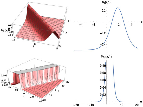
Figure 1.
The 2D, and 3D plots of solitary wave perspective view of U1(x, t) and W1(x, t).
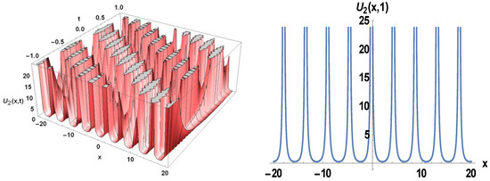
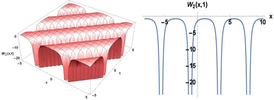
Figure 2.
The 2D, and 3D plots of solitary wave of perspective view of U2(x, t) and W2(x, t).
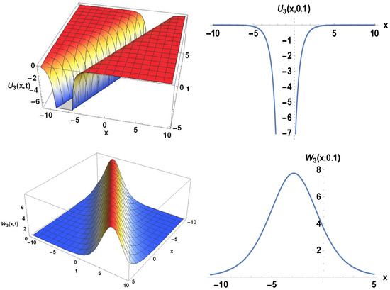
Figure 3.
The 2D, and 3D plots of solitary wave of perspective view of U3(x, t) and W3(x, t).
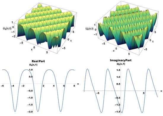
Figure 4.
The real and imaginary parts of 2D, and 3D plots of the solitary wave of perspective view of U6(x,t).
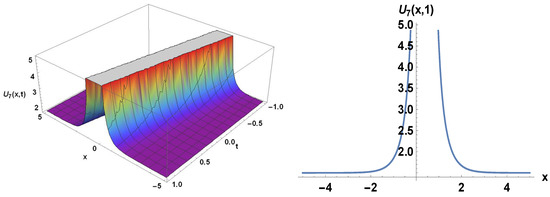
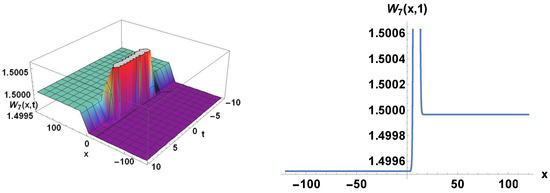
Figure 5.
The 2D, and 3D, plots of the solitary wave perspective view of U7(x, t) and W7(x, t).
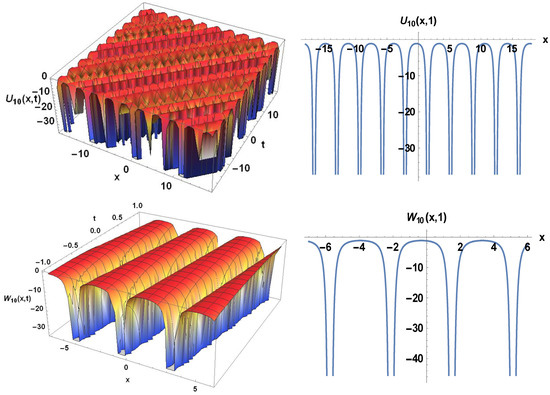
Figure 6.
The 3D, and 2D plots of the solitary wave perspective view of U10(x, t) and W10(x, t).
5. Conclusions
The modified exp-function method has been successfully applied in this article to develop the analytical solutions to the Riemann wave equations. For each of the analyzed equations with some unknown parameters, we have constructed general solitary wave solutions. For the definite values of the parameters, some existing solutions from the literature are identified as well as some new solutions. Diverse varieties of solitary waves, videlicet bell shapes, reduced bell shapes, compacton shapes, singular kink shapes, flat kink shapes, smooth singular shapes, and other soliton solutions are among the established solutions. The behaviour of the solitary waves in relation to time and space has been illustrated graphically. This useful method can be applied to investigate different NLEE types that regularly occur in a variety of scientific and practical applications. The discovered solutions will aid in the investigation of issues in mathematical physics and engineering. The physical interpretation of the proposed solutions and their actual implementation in practice will be looked into in this study.
Author Contributions
Conceptualization, A. and N.A.S.; methodology, M.S.; software, B.A.; validation, M.S., B.A. and J.D.C.; formal analysis, A. and N.A.S.; investigation, J.D.C.; resources, B.A.; data curation, A. and N.A.S.; writing—original draft preparation, M.S. and B.A.; writing—review and editing, A., N.A.S. and J.D.C.; funding acquisition, J.D.C. All authors have read and agreed to the published version of the manuscript.
Funding
This research received no external funding.
Data Availability Statement
Not Applicable.
Acknowledgments
This work was supported by the Technology Innovation Program (20018869, Development of Waste Heat and Waste Cold Recovery Bus Air-conditioning System to Reduce Heating and Cooling Load by 10%) funded By the Ministry of Trade, Industry & Energy (MOTIE, Republic of Korea).
Conflicts of Interest
The authors declare no conflict of interest.
References
- Helal, M.A.; Seadawy, A.R. Benjamin-Feir-instability in nonlinear dispersive waves. Comput. Math. Appl. 2012, 64, 3557–3568. [Google Scholar] [CrossRef]
- Seadawy, A.R. Exact Solutions of a two-dimensional nonlinear Schrodinger equation. Appl. Math. Lett. 2012, 25, 687–691. [Google Scholar] [CrossRef]
- Kudryashov, N.A. Painleve analysis and exact solutions of the fourth order equation for description of nonlinear waves. Commun. Nonlinear Sci. Numer. Simul. 2015, 28, 1–9. [Google Scholar] [CrossRef]
- Cattani, C.; Sulaiman, T.A.; Baskonus, H.M.; Bulut, H. Solitons in an inhomogeneous Murnaghan’s rods. Eur. Phys. J. Plus 2018, 133, 228. [Google Scholar] [CrossRef]
- Zhao, Y.M. The F-expansion method and its application for finding new exact solutions to the Kudryashov-Sinelshchikov equation. J. Appl. Math. 2013, 7, 895760. [Google Scholar] [CrossRef]
- Bulut, H.; Pandir, Y.; Demiray, S.T. Exact solutions of time fractional KdV equation by using the generalized Kudryashov method. Int. J. Model. Optim. 2014, 4, 315–320. [Google Scholar] [CrossRef]
- Helal, M.A.; Seadawy, A.R. Exact soliton solutions of an D-dimensional nonlinear Schrodinger equation with damping and diffusive terms. Z. Angew. Math. Phys. (ZAMP) 2011, 62, 839–847. [Google Scholar] [CrossRef]
- Seadawy, A.R. New exact solutions for the KdV equation with higher order nonlinearity by using the variational method. Comput. Math. Appl. 2011, 62, 3741–3755. [Google Scholar] [CrossRef]
- Triki, H.; Wazwaz, A.M. Bright and dark soliton solutions for a k(m, n) equation with time dependent coefficients. Phys. Lett. A 2009, 373, 2162–2165. [Google Scholar] [CrossRef]
- Wang, M.L.; Zhou, Y.B.; Li, Z.B. Application of a homogeneous balance method to exact solutions of nonlinear equations in mathematical physics. Phys. Lett. A 1996, 216, 67–75. [Google Scholar] [CrossRef]
- Abdusalam, H.A. On an improved complex tanh-function method. Int. J. Nonlinear Sci. Numer. Simul. 2005, 6, 99–106. [Google Scholar] [CrossRef]
- Helal, M.A.; Seadawy, A.R. Variational method for the derivative nonlinear Schrodinger equation with computational applications. Phys. Scr. 2009, 80, 350–360. [Google Scholar] [CrossRef]
- Khater, A.H.; Callebaut, D.K.; Helal, M.A.; Seadawy, A.R. Variational method for the nonlinear dynamics of an elliptic magnetic stagnation line. Eur. Phys. J. D 2006, 39, 237–245. [Google Scholar] [CrossRef]
- Jaradat, I.; Alquran, M.; Momani, S.; Biswas, A. Dark and singular optical solutions with dual-mode nonlinear Schrodinger’s equation and Kerr-law nonlinearity. Optik 2018, 172, 822–825. [Google Scholar] [CrossRef]
- He, J.H.; Wu, X.H. Exp-function methon method for nonlinear wave equations. Chaos Soliton Fract. 2006, 30, 700–708. [Google Scholar] [CrossRef]
- Akbar, M.A.; Ali, N.M. The improved F-expansion method with Riccati equation and its application in mathematical physics. Cogent Math. Stat. 2017, 41, 282–577. [Google Scholar] [CrossRef]
- Ma, W.X. N-soliton solution and the Hirota condition of a (2 + 1)-dimensional combined equation. Math. Comput. Simul. 2021, 190, 270–279. [Google Scholar] [CrossRef]
- Liu, Y.; Wen, X.Y.; Wang, D.S. The N-soliton solution and localized wave interaction solutions of the (2 + 1)-dimensional generalized Hirota-Satsuma-Ito equation. Comput. Math. Appl. 2019, 77, 947–966. [Google Scholar] [CrossRef]
- Liu, Y.; Wang, D.S. Exotic wave patterns in Riemann problem of the high-order Jaulent–Miodek equation: Whitham modulation theory. Stud. Appl. Math. 2022, 149, 588–630. [Google Scholar] [CrossRef]
- Jawad, A.J.M.; Johnson, S.; Yildirim, A.; Kumar, S.; Biswas, A. Soliton solutions to the coupled nonlinear wave equations in (2 + 1) dimensions. Indian J. Phys. 2013, 87, 281–287. [Google Scholar] [CrossRef]
- Spatschek, K.H.; Shukla, P.K. Nonlinear interaction of magneto-sound wave with whistler turbulence. Radio Sci. 1978, 13, 211–214. [Google Scholar] [CrossRef]
- Khater, A.H.; Callebaut, D.K.; Seadawy, A.R. General soliton solutions of an n-dimensional complex Ginzburg–Landau equation. Phys. Scr. 2000, 62, 353. [Google Scholar] [CrossRef]
- Shakeel, M.; Attaullah; El-Zahar, E.R.; Shah, N.A.; Chung, J.D. Generalized exp-function method to find closed form solutions of nonlinear dispersive modified Benjamin–Bona–Mahony equation defined by seismic sea waves. Mathematics 2022, 10, 1026. [Google Scholar] [CrossRef]
- Shakeel, M.; Attaullah; Shah, N.A.; Chung, J.D. Modified Exp-Function Method to Find Exact Solutions of Ionic Currents along Microtubules. Mathematics 2022, 10, 851. [Google Scholar]
- Shakeel, M.; Mohyud-Din, S.T.; Iqbal, M.A. Closed form solutions for coupled nonlinear Maccari system. Comput. Math. Appl. 2018, 76, 799–809. [Google Scholar] [CrossRef]
- Rani, A.; Shakeel, M.; Alaoui, K.M.; Zidan, A.M.; Shah, N.A.; Junsawang, P. Application of the Exp(−φ(ξ))-expansion method to find the soliton solutions in biomembranes and nerves. Mathematics 2022, 10, 3372. [Google Scholar] [CrossRef]


Publisher’s Note: MDPI stays neutral with regard to jurisdictional claims in published maps and institutional affiliations. |
© 2022 by the authors. Licensee MDPI, Basel, Switzerland. This article is an open access article distributed under the terms and conditions of the Creative Commons Attribution (CC BY) license (https://creativecommons.org/licenses/by/4.0/).