Shape Phase Transitions in Even–Even ^176–198Pt: Higher-Order Interactions in the Interacting Boson Model ^†

Abstract

Dynamical symmetry plays a dominant role in the interacting boson model in elucidating nuclear structure, for which group theoretical or algebraic techniques are powerful. In this work, the higher-order interactions required in describing triaxial deformation in the interacting boson model are introduced to improve the fitting results to low-lying level energies, $B(E2)$ values and electric quadrupole moments of even–even nuclei. As an example of the model application, the low-lying excitation spectra and the electromagnetic transitional properties of even–even ^176−198Pt are fitted and compared to the experimental data and the results of the consistent-Q formalism. It is shown that the results obtained from the model are better than those of the original consistent-Q formalism, indicating the importance of the higher-order interactions in describing the structure and the shape phase evolution of these nuclei.

1. Introduction

It has so far been shown that the interacting boson model (IBM) proposed by Arima and Iachello [1,2,3,4,5] is very successful in describing low-lying spectra of medium and heavy mass even–even nuclei [6,7]. Shape phase evolution in these nuclei has also been extensively investigated [8,9,10,11]. The dynamical symmetry concept plays a dominant role in the interacting boson model, for which group theoretical or algebraic techniques are powerful. The model with no distinction between neutrons and protons is called IBM-1, which is simply called IBM in this paper. In addition, as another application of symmetry concept in nuclear structure, it has been shown very recently that the charge and matter radii of ${}^{4,6,8}$He and the sizes of the self-conjugate A = 4n nuclei calculated from the quantitative geometrical thermodynamics in taking the symmetry of alpha-particle into account agree closely with observed values [12].

In the IBM, an even–even nucleus is treated as an inert closed-shell core plus valence nucleons or holes outside of the core. It is assumed that the valence-like nucleons are paired with angular momentum l = 0 or 2, and can be approximately treated as s-bosons and d-bosons. Hence, the IBM is equivalent to the shell model confined within the neutron and proton valence shells truncated within S- and D-pair subspace [13] without Pauli exclusion. Since the total number of valence nucleons is a conserved quantity, the total number of bosons in the IBM is an invariant. The single s-boson and five d-boson creation operators denoted as $\{s^{†},d_{\nu }^{†}\}$ ($\nu =-2,-1,\cdots ,2$) form a basis of the vector representation of the U(6) group [1,6]. Thus, the model Hamiltonian can be realized by 36 generators $\{s^{†}{d}_{\nu },d_{\nu }^{†}s,d_{\nu }^{†}{d}_{{\nu }^{\prime }},s^{†}s\}$ of the U(6) group after the second quantization procedure, and must be kept as an SO(3) scalar due to the rotational symmetry of nuclei. As the consequence, for the given total number of bosons N, all possible linearly independent N-boson states form the symmetric irreducible representation (irrep) $[N,0]$ of the U(6) group. Due to the SO(3) invariance, the N-boson states organized as the basis vectors of the irrep $[N,0]$ of U(6) classified in a group chain U(6)⊃SO(3) are convenient to be used in diagonalizing the model Hamiltonian.

In previous IBM descriptions of Pt isotopes, the model Hamiltonian only contains one- and two-body interactions [14,15]. However, electric quadrupole moments of low-lying states near the O(6) limit are too small due to the O(6) selection rules, which is obviously inconsistent to the experimental results. Besides the three- and four-body interactions required to describe triaxiality, an exponential modification to the strength of the quadrupole–quadrupole interaction has been proposed [16,17], which improves the fitting quality of low-lying excited states, B(E2) values and electric quadrupole moments [17]. Based on the CQ Hamiltonian, we make use of the general quadrupole operators $Q_{\nu }(\chi )$ in replacing the SU(3) generators $Q_{\nu }(-\sqrt{7}/2)$ in the rigid triaxial rotor descriptions [18,19] or the $\gamma$-soft rotor descriptions with the O(6) generators $Q_{\nu }(0)$ [17] to construct a more general soft rotor model Hamiltonian, which is called the modified soft rotor model. The modified soft rotor model Hamiltonian includes the general quadrupole–quadrupole interaction, the three- and four-body terms, and the d-boson number operator. Hence, the model can be used to describe medium and heavy mass even–even nuclei with better fitting quality. As an example of the model application, some low-lying positive parity level energies, B(E2) values and electric quadrupole moments of some low-lying states in the even–even ${}^{176–198}$Pt are fitted and compared to the experimental data and the results of the consistent-Q formalism.

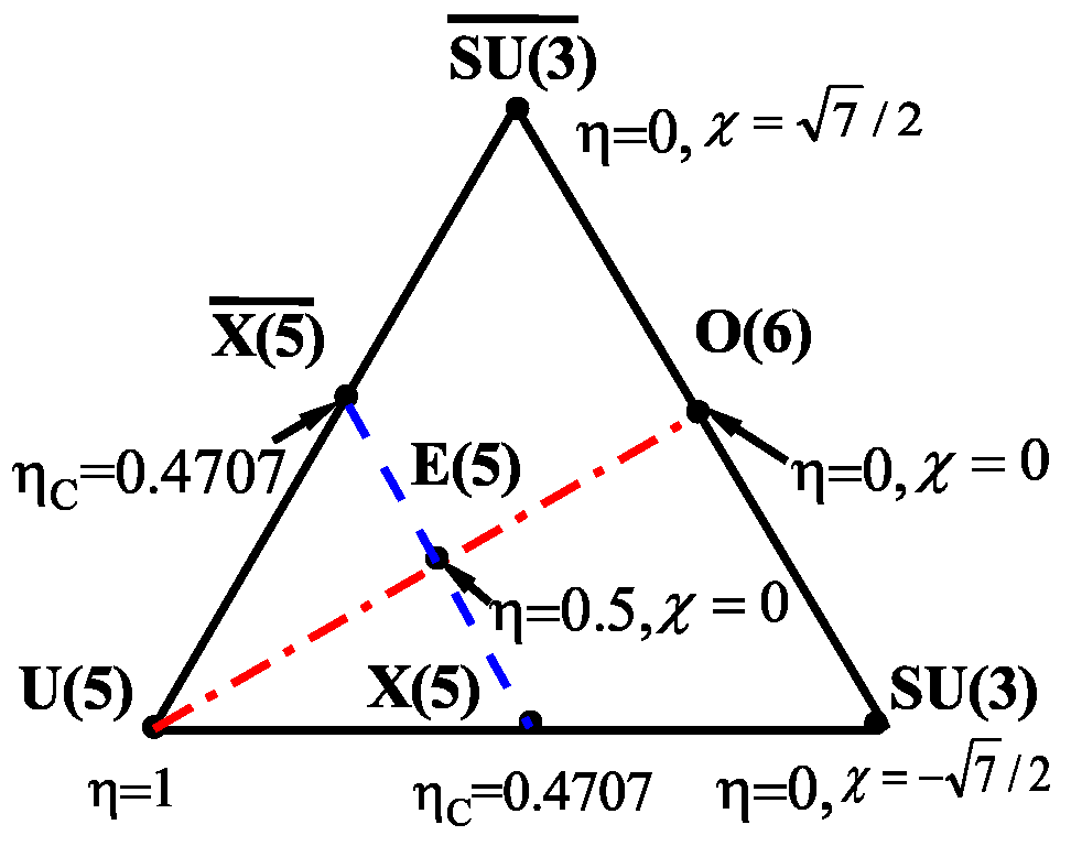
2. The CQ Formalism and Its Extension

The simplest IBM Hamiltonian contains only one- and two-body terms, with other possible higher-order terms neglected. The compact form, in which the quadrupole operators in both the Hamiltonian and the E2 operator are taken to be the same, is called consistent-Q (CQ) formalism [20,21]. In the CQ formalism, the model Hamiltonian is expressed as [15,22]

$$\begin{array}{cc}\hfill {\widehat{H}}_{\mathrm{CQ}}=& c\left(\eta {\widehat{n}}_d+\frac{\eta -1}{4N}Q(\chi )·Q(\chi )\right),\hfill \end{array}$$

(1)

where N is the total boson number, c is the scaling parameter, ${\widehat{n}}_d={\Sigma }_{\nu }{d}_{\nu }^{†}{d}_{\nu }$ and $Q_{\nu }(\chi )=s^{†}{\tilde{d}}_{\nu }+d_{\nu }^{†}s+\chi {(d^{†}\times \tilde{d})}_{\nu }^{(2)}$ with ${\tilde{d}}_{\nu }={(-)}^{\nu }{d}_{-\nu }$, which are the d-boson number operator and quadrupole operator, respectively, ${(d^{†}\times \tilde{d})}_{\nu }^{(k)}$ stands for the tensor coupling, and the parameters $\eta \in [0,1]$ and $\chi \in [-\frac{\sqrt{7}}{2}$, $\frac{\sqrt{7}}{2}]$. When the SO(3) irreps characterized by the quantum numbers of the angular momentum of the bosons are embedded within the irrep $[N,0]$ of U(6), there are three and only three possible ways [6]:

$$\mathrm{U}(6)\supset \begin{array}{cc}& \mathrm{U}(5)\supset \mathrm{O}(5)\\ & \mathrm{O}(6)\supset \mathrm{O}(5)\\ & \mathrm{SU}(3)\mathrm{or}\overline{\mathrm{SU}(3)}\end{array}\supset \mathrm{SO}(3),$$

(2)

where U(5) is generators by ${(d^{†}\times \tilde{d})}_{\nu }^{(k)}$ ($k=0,1\cdots ,4$), $\mathrm{O}(6)$ is generated by $\{L_{{\nu }^{\prime }}=\sqrt{10}{(d^{†}\times \tilde{d})}_{{\nu }^{\prime }}^{(1)},{(d^{†}\times \tilde{d})}_{\mu }^{(3)},Q_{\nu }(0)\}$, in which $L_{{\nu }^{\prime }}$ (${\nu }^{\prime }=-1,0,+1$) are the total angular momentum operators of the bosons, $\mathrm{SU}(3)$ is generated by $\{L_{{\nu }^{\prime }},Q_{\nu }(-\sqrt{7}/2)\}$, while $\overline{\mathrm{SU}(3)}$ is generated by $\{L_{{\nu }^{\prime }},Q_{\nu }(+\sqrt{7}/2)\}$. It should be noted that $\overline{\mathrm{SU}(3)}$ is isomorphic to SU(3), but the generators of SU(3) are obviously different from those of $\overline{\mathrm{SU}(3)}$ with different geometric explanations shown in the following. When $\eta =1$, the basis vectors of U(6)⊃U(5)⊃O(5)⊃ SO(3) are eigenstates of the Hamiltonian (1), which is called the U(5) (spherical) vibrational limit of the model. In the U(5) limit, the nuclear shape is spherical with small $\beta$-vibration. When $\eta =0$ and $\chi =0$, the eigenstates of the Hamiltonian (1) are the basis vectors of U(6)⊃O(6)⊃O(5)⊃ SO(3), which is called the O(6) ($\gamma$-unstable) limit. In the O(6) limit, the nuclear shape is an ellipsoid with indefinite (unstable) triaxiality, where the triaxiality $0^{\circ }\le \gamma \le {60}^{\circ }$ and the dimensionless quadrupole deformation parameter $\beta$ are the Bohr variables to describe the shape of an ellipsoid used in the collective model [23]. When $\eta =0$ and $\chi =\mp \sqrt{7}/2$, the eigenstates of the Hamiltonian (1) are the basis vectors of U(6)⊃SU(3)⊃ SO(3) with the minus sign or U(6)⊃$\overline{\mathrm{SU}(3)}$⊃ SO(3) with the plus sign. The former is called the SU(3) limit, in which the nuclear shape is an axially deformed prolate ellipsoid with $\gamma =0^{\circ }$, while the latter is called the $\overline{\mathrm{SU}(3)}$ limit, in which the nuclear shape is an axially deformed oblate ellipsoid with $\gamma ={60}^{\circ }$. In the three limiting cases, the Hamiltonian (1) is invariant under the U(5), O(6), SU(3) [$\overline{\mathrm{SU}(3)}$] transformation, respectively. Therefore, U(5), O(6), and SU(3) ($\overline{\mathrm{SU}(3)}$) are the dynamical symmetry groups in the three limiting cases, respectively. Accordingly, within the CQ formalism, the shape of a nucleus is determined by the parameters $(\eta ,\chi )$, which can be represented vividly by the extended Casten triangle [8,9] shown in Figure 1, where the three vertices are labeled by the three limits of the CQ Hamiltonian, the U(5)–SU(3) and U(5)–$\overline{\mathrm{SU}(3)}$ sides are the connection of the $(\eta =1,\chi =\mp \sqrt{7}/2)$ and $(\eta =0,\chi =\mp \sqrt{7}/2)$ vertices, while the SU(3)–$\overline{\mathrm{SU}(3)}$ side is the connection of the $(\eta =0,\chi =-\sqrt{7}/2)$ and $(\eta =0,\chi =\sqrt{7}/2)$ vertices, and the O(6) point with $(\eta =0,\chi =0)$ is on the SU(3)–$\overline{\mathrm{SU}(3)}$ side. The above correspondence between the special IBM parameters and the shape defined by the Bohr variables $(\beta ,\gamma$) in the collective model was established by using the coherent state formalism [24,25,26]. By using the coherent state formalism, it is further shown that, besides the limiting cases, the point at $(\eta =0.5,\chi =0)$ along the U(5)–O(6) line shown in Figure 1 is the critical point of the U(5) (spherical) to the O(6) ($\gamma$-unstable) shape phase transition in the large-N limit, which is called the E(5) dynamical symmetry in the collective model [27]. Similarly, the point at $(\eta =0.4707,\chi =\mp \sqrt{7}/2)$ on the U(5)–SU(3) [$\overline{\mathrm{SU}(3)}$] side is the critical point of the U(5) (spherical) to the SU(3) [$\overline{\mathrm{SU}(3)}$] (axially deformed) shape phase transition in the large-N limit, which is called the X(5) [$\overline{\mathrm{X}(5)}$] dynamical symmetry in the collective model [28]. Anyway, the extended Casten triangle elucidates possible nuclear shapes and their evolutions with the variation of the model parameters $\eta$ and $\chi$ in the CQ formalism, except that the triaxial shapes are missing.

Since the IBM Hamiltonian with up to two-body interactions is unable to describe stable triaxial deformation, in order to reproduce a $\gamma$-rigid triaxial shape, higher-order terms have to be included [29,30,31,32,33,34,35]. For example, the IBM Hamiltonian with ${[{[d^{†}\times d^{†}]}^{(k)}\times d^{†}]}^{(3)}·{[{[\tilde{d}\times \tilde{d}]}^{(k^{\prime })}\times \tilde{d}]}^{(3)}$ term can give rise of the stable triaxial deformation [30]. It is shown that the double $\gamma$ anharmonic vibration reflects the importance of three-body interaction [31]. A similar conclusion was also made in [32,33]. Moreover, the O(6) symmetry-conserving higher-order interactions were investigated [34]. The influences of symmetry-conservation higher-order interactions in the $\beta$- and $\gamma$-band of the IBM SU(3) limit were also discussed in detail [35], where the $\beta$-band refers to the excited levels following the rotational level pattern established on the first excited $0^{+}$ level, and $\gamma$-band refers to those established on the second excited $2^{+}$ level in the collective model, in which the $\beta$-band head (the first excited $0^{+}$ level) is due to the $\beta$-vibration excitation, while the $\gamma$-band head (the second excited $2^{+}$ level) is due to the excitation related to the $\gamma$-vibration energy. In this case, the even–even nucleus concerned is assumed to be axially deformed with small $\beta$- and $\gamma$-vibrations. The situation in the transitional nuclei is different because the nuclear shape in this case is not prolate and often $\gamma$-unstable. Therefore, levels established on the second excited $2^{+}$ level in transitional nuclei are often called quasi $\gamma$-band. In addition, it is shown that the rotational spectra, which is the result of the two-body SU(3) quadrupole–quadrupole interaction, can also be generated by using the triple coupling scalar of the O(6) quadrupole operator [36]. Although the two descriptions can offer similar rotational spectra, the electromagnetic transitional properties are quite different [37]. The model with the triple coupling scalar of the O(6) quadrupole operators was also used to describe the triaxial deformation and the prolate to oblate shape phase evolution [38].

In the IBM, the SU(3) implementation of a rigid triaxial rotor was established [18,19] based on the early observation [39,40]. Specifically, a general rotor Hamiltonian is given as

$$H_{\mathrm{rot}}=A_1{L}_1^2+A_2{L}_2^2+A_3{L}_3^2,$$

(3)

where $L_{\alpha }$ is the projection of the angular momentum onto the $\alpha$-th body-fixed principal axis, and $A_{\alpha }$ is the corresponding inertia parameter, which can be expressed in terms of the Bohr variables $(\beta ,\gamma )$ in the collective model [23]. The asymmetry parameter $\kappa$ related to the inertia ellipsoid is defined by

$$\kappa =(2A_1-A_2-A_3)/(A_3-A_2).$$

(4)

The rotor is prolate when $A_1=A_2<A_3$ with $\kappa =-1$; oblate when $A_2<A_1=A_3$ with $\kappa =+1$; and most asymmetric when $A_1=\frac{1}{2}(A_2+A_3)$ with $\kappa =0$ [39,40]. It is obvious that the shape referred to here is the dynamical shape determined by the inertia parameters along the principal axes, though it coincides with the geometric shape of the rotor in most cases. The algebraic image of the general rotor Hamiltonian (3) can be realized [39,40] by rewriting $H_{\mathrm{rot}}$ in a frame-independent form by introducing and using the angular momentum $L_u$ and the mass quadrupole tensor operators ${\mathcal{Q}}_u$ with

$$\begin{array}{ccc}\hfill & & L_u=\int \rho (\overrightarrow{r}){(\overrightarrow{r}\times \overrightarrow{v})}_{u}d\tau ,\hfill \\ & & {\mathcal{Q}}_{\nu }=\sqrt{16\pi /5}\int \rho (\overrightarrow{r})r^2{Y}_{2\nu }(\Omega )d\tau ,\hfill \end{array}$$

(5)

where $\rho (\overrightarrow{r})$ is the nuclear mass density, and the integration is over the whole nuclear volume. It can be proven that these operators satisfy the following commutation relations:

$$\begin{array}{ccc}\hfill & & [L_u,L_{\nu }]=-\sqrt{2}\langle 1u,1v|1u+v\rangle L_{u+\nu },\hfill \\ & & [L_u,{\mathcal{Q}}_{\nu }]=-\sqrt{6}\langle 1u,2v|2u+v\rangle {\mathcal{Q}}_{u+\nu },\hfill \\ \hfill & & [{\mathcal{Q}}_{\nu },{\mathcal{Q}}_{{\nu }^{\prime }}]=0,\hfill \end{array}$$

(6)

which thus generate the dynamical symmetry group of the quantum rotor, the semidirect product group $T_5{\otimes }_s\mathrm{SO}(3)$. In the body-fixed principal-axial system, one has [39,40]

$$\begin{array}{ccc}\hfill & & L^2=L_1^2+L_2^2+L_3^2,\hfill \\ & & X_3=\sum _{\alpha \beta }{L}_{\alpha }{\mathcal{Q}}_{\alpha \beta }{L}_{\beta }={\lambda }_1{L}_1^2+{\lambda }_2{L}_2^2+{\lambda }_3{L}_3^2,\hfill \\ \hfill & & X_4=\sum _{\alpha \beta \gamma }{L}_{\alpha }{\mathcal{Q}}_{\alpha \beta }{\mathcal{Q}}_{\beta \gamma }{L}_{\gamma }={\lambda }_1^2{L}_1^2+{\lambda }_2^2{L}_2^2+{\lambda }_3^2{L}_3^2,\hfill \end{array}$$

(7)

where $L_{\alpha }$ and ${\mathcal{Q}}_{\alpha \beta }$ are the Cartesian form of $L_u$ and ${\mathcal{Q}}_u$ introduced in (5), and ${\lambda }_{\alpha }$ are the eigenvalues of $\mathcal{Q}$ in the body-fixed principal-axial system: $\langle {\mathcal{Q}}_{\alpha \beta }\rangle ={\lambda }_{\alpha }{\delta }_{\alpha \beta }$. From (7), we have

$$L_{\alpha }^2=[({\lambda }_1{\lambda }_2{\lambda }_3)L^2+{\lambda }_{\alpha }^2{X}_3^c+{\lambda }_{\alpha }{X}_4^c]/(2{\lambda }_{\alpha }^3+{\lambda }_1{\lambda }_2{\lambda }_3).$$

(8)

Thus, the rotor Hamiltonian (3) can be expressed as [39,40]

$$H_{\mathrm{rot}}=a{L}^2+b{X}_3+b^{\prime }{X}_4,$$

(9)

where the parameters a, b, and $b^{\prime }$ depend on the inertia parameters $A_{\alpha }$ and the eigenvalues of $\mathcal{Q}$ with

$$\begin{array}{ccc}\hfill & & a=\sum _{\alpha }{z}_{\alpha }{A}_{\alpha },z_{\alpha }={\lambda }_1{\lambda }_2{\lambda }_3/D_{\alpha },\hfill \\ & & b=\sum _{\alpha }{b}_{\alpha }{A}_{\alpha },b_{\alpha }={\lambda }_{\alpha }^2/D_{\alpha },\hfill \\ \hfill & & b^{\prime }=\sum _{\alpha }{c}_{\alpha }{A}_{\alpha },c_{\alpha }={\lambda }_{\alpha }/D_{\alpha },\hfill \end{array}$$

(10)

and

$$D_{\alpha }=2{\lambda }_{\alpha }^3+{\lambda }_1{\lambda }_2{\lambda }_3.$$

(11)

The expression (9) was used to make the SU(3) realization of the rotor Hamiltonian in the IBM framework [18,19]. In the SU(3) realization [18,19], the mass quadrupole tensor components ${\mathcal{Q}}_{\nu }$ is replaced by the SU(3) generators $Q_{\nu }(-\sqrt{7}/2)$. Hence, besides the $L^2$ term, the high order terms

$$\begin{array}{cc}\hfill & X_3={(L\times Q(-\sqrt{7}/2)\times L)}^{(0)},\\ & X_4={\left({(L\times Q(-\sqrt{7}/2))}^{(1)}\times (L\times Q{(-\sqrt{7}/2)}^{(1)}\right)}^{(0)}\end{array}$$

(12)

should be included in the Hamiltonian to describe a rigid rotor with fixed triaxiality [18,19,39]. Recently, it has been further shown that the IBM with the SU(3) third-order term can be used to describe the oblate shape [41] and to explain the B(E2) anomaly in some neutron deficient nuclei [42,43,44]. It should be pointed out that the inertia parameters along the principal axes are indefinite due to the fact that $\gamma$ is a variable in the O(6) limit, which answers why it is called $\gamma$-unstable, while the inertia parameters along the three principal axes are fixed when the rotor is realized in the SU(3) limit with nonzero b and $b^{\prime }$ in (9) corresponding to the rigid triaxial ($\gamma$-rigid) case.

Since the triaxiality of the rotor is always fixed when $X_3$ and $X_4$ are realized by using the SU(3) generators $Q_{\nu }(-\sqrt{7}/2)$ [19] or $\gamma$-indefinite (unstable) when the O(6) generators $Q_{\nu }(0)$ are used in $X_3$ and $X_4$, in order to describe a more general situation of triaxial nuclei, we use the general quadrupole operators $Q_{\nu }(\chi )$ with $\chi \in [-\sqrt{7}/2,\sqrt{7}/2]$ to construct the high order terms $X_3$ and $X_4$, with which the model is called modified soft rotor. The modified soft rotor model covers not only the rigid triaxial case with $\chi =\mp \sqrt{7}/2$ and the $\gamma$-indefinite (unstable) case with $\chi =0$, but also the intermediate (soft) case with $\chi \in (-\sqrt{7}/2,0)\bigcup (0,\sqrt{7}/2)$.

3. The Modified Soft Rotor Model

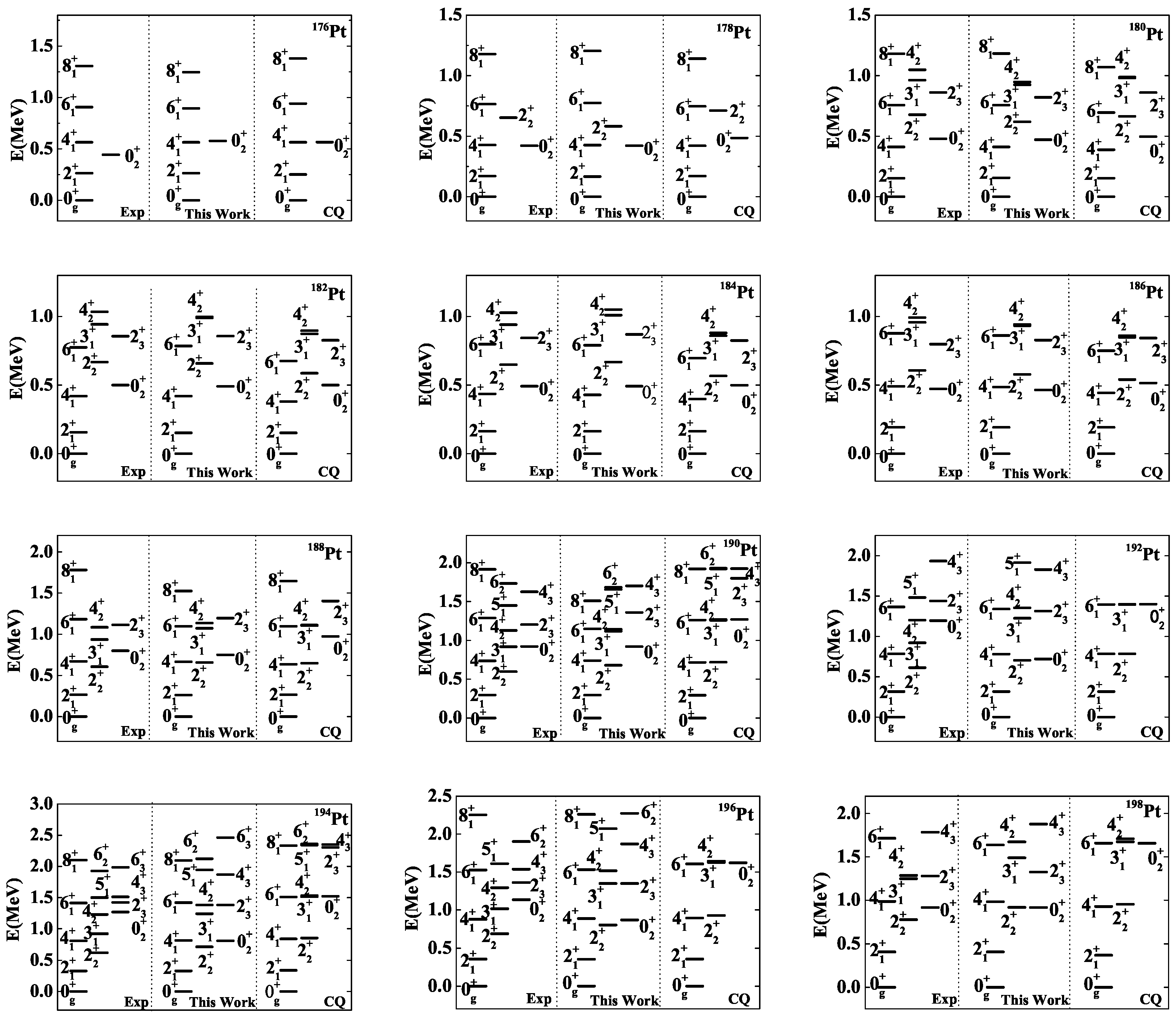
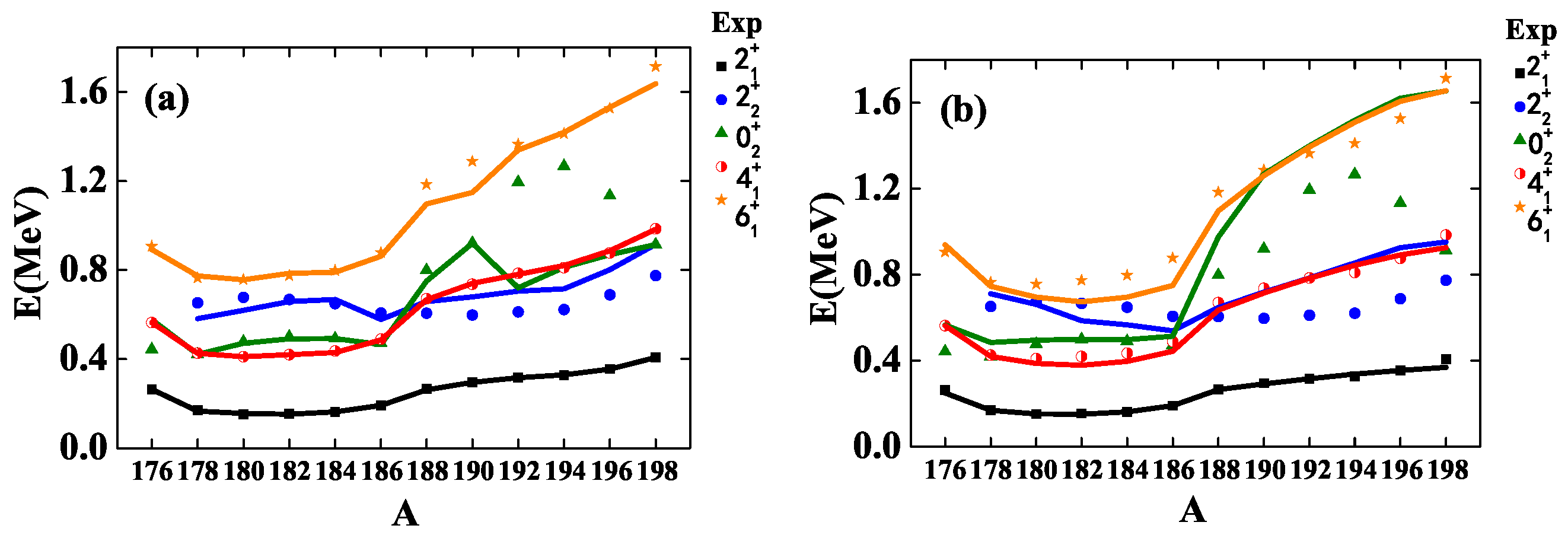
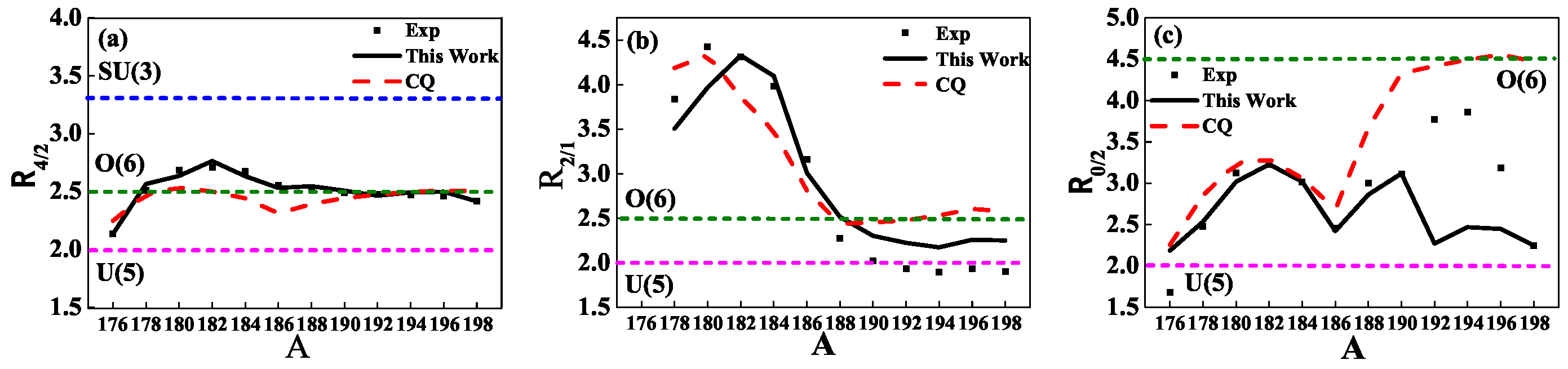
Based on the CQ Hamiltonian, in addition to the d-boson number operator and quadrupole–quadrupole interaction, the three- and four-body terms are introduced to cover the emergence of triaxiality. Thus, the modified soft rotor model Hamiltonian is expressed as

$$\begin{array}{cc}\hfill \widehat{H}=& c_0(\eta {\widehat{n}}_d+\frac{\eta -1}{4N}{e}^{\xi Q·Q}Q(\chi )·Q(\chi )+\frac{2a_1}{N^2}{\left(\widehat{L}\times Q(\chi )\times \widehat{L}\right)}^{(0)}\hfill \\ & +\frac{4a_2}{N^3}{\left({(\widehat{L}\times Q(\chi ))}^{(1)}\times {(\widehat{L}\times Q(\chi ))}^{(1)}\right)}^{(0)}+\frac{a_3}{4N}\widehat{L}·\widehat{L}),\hfill \end{array}$$

(13)

where $\xi$, $a_1$, $a_2$, $a_3$ are the dimensionless real parameters, and $Q_{\nu }\equiv Q_{\nu }(-\sqrt{7}/2)$ in the exponential of the second term is adopted, which is introduced to reduce the excitation energies of the eigenstates with higher angular momentum, while the other terms are the same as those shown in (1). The microscopic shell model foundation of these high-order interactions is shown in [16]. Most importantly, instead of $Q_{\nu }(-\frac{\sqrt{7}}{2})$ for the rigid rotor in the SU(3) limit or $Q_{\nu }(0)$ of the $\gamma$-unstable rotor in the O(6) limit, the general quadrupole operators $Q_{\nu }(\chi )$ with $\chi \in [-\frac{\sqrt{7}}{2}$, $\frac{\sqrt{7}}{2}]$ are used in the three- and four-body terms. The Hamiltonian (13) not only maintains the consistency to the CQ Hamiltonian, but also covers the emergence of triaxiality, so it should provide a better description of structural evolution of medium and heavy mass nuclei.

It should be noted that the full set of the basis vectors of any group chain shown in (2) is complete. The Hamiltonian (13) is diagonalized in theU(6)⊃SU(3)⊃SO(3)⊃SO(2) basis, of which the basis vectors are denoted as $\{|N(\lambda \mu )\kappa ,LM\rangle \}$, where $(\lambda ,\mu )$ labels the irreducible representation of the SU(3) group, $\kappa$ is the additional quantum number required in the reduction SU(3) ↓ SO(3), L is the quantum number of the angular momentum, and M is the quantum number of the angular momentum projection. Thus, the eigenstates of the Hamiltonian (13) can be expressed as

$$\begin{array}{c}\hfill |N{L}_{\varsigma }\rangle =\sum _{(\lambda \mu )\kappa }{C}_{(\lambda \mu )\kappa }^{L_{\varsigma }}|N(\lambda \mu )\kappa L\rangle ,\end{array}$$

(14)

where $\varsigma$ labels different eigenstates, but with the same L, and $C_{(\lambda \mu )\kappa }^{L_{\varsigma }}$ is the expansion coefficient. As with the CQ formalism, the E2 transition operators is defined as

$$\begin{array}{c}\hfill T_{\nu }(E2)=q_2{Q}_{\nu }(\chi ),\end{array}$$

(15)

where $q_2$ is the effective boson charge-related parameter. Hence, the B(E2) values are given by

$$\begin{array}{c}\hfill B(E2;L_{\varsigma }\to L_{{\varsigma }^{\prime }}^{\prime })=\frac{1}{2L+1}|\langle N{L}_{{\varsigma }^{\prime }}^{\prime }\parallel T(E2)\parallel N{L}_{\varsigma }{\rangle |}^2,\end{array}$$

(16)

in which the reduced matrix element $\langle N{L}_{{\varsigma }^{\prime }}^{\prime }\parallel T(E2)\parallel N{L}_{\varsigma }\rangle$ is defined in terms of the 3j-symbol according to the Wigner–Eckart theorem. A Fortan code of this work is written based on the results shown in [15,45], in which the $\mathrm{SU}(3)\supset \mathrm{SO}(3)$ Wigner coefficients are taken from the Draayer–Akiyama code [46].

4. Shape Phase Transition in ${}^{\mathbf{176}–\mathbf{198}}$ Pt

Shape phase transition and possible cross-shell excitations in even–even Pt isotopes with mass number $172\le A\le 194$ have been investigated. In [14,15,47], the analysis on the shape phase transition behaviors from the prolate to $\gamma$-unstable then to the oblate shape in several lower excited states of the even–even Pt isotopes was made by using the CQ Hamiltonian without configuration mixing. The IBM-2 model calculation for the even–even Pt isotopes was reported in [48], in which only the level energies up to $8_1^{+}$ state in the yrast band and a few excited states in the quasi-$\beta$ and quasi-$\gamma$ band and the electric quadrupole moment of $2_1^{+}$ state were fitted, where the yrast band consists of a series of the lowest energy levels for given quantum number of the angular momentum. In these Pt isotopes, configuration mixing with intruder excitation is likely to occur. A comparison and analysis of the model with and without configuration mixing are made in [49], in which possible intruder states in the excitation spectra of Pt isotopes are pointed out. In [17], the configuration mixing calculation of the low-lying spectrum of ${}^{194}$Pt is carried out in the $\gamma$-soft rotor model, in which the O(6) quadrupole operators are used. The results show that the $\gamma$-soft rotor model fitting results to the low-lying level energies and the electric quadrupole moments are much improved.

As an example of the modified soft rotor model application, the low-lying excitation spectra and the electromagnetic transitional properties of even–even ${}^{176–198}$Pt are fitted and compared to the experimental data and the results of the consistent-Q formalism, in which the configuration mixing is not considered for simplicity.

Since the IBM is equivalent to the valence shell model calculation, it is only suitable to describe low-lying positive parity states of medium and heavy even–even nuclei except for $1^{+}$ states, which are due to the proton–neutron coupling or cross-shell particle-hole excitation. Hence, in this work, except $1^{+}$ levels, only low-lying positive-parity level energies and related electromagnetic properties of even–even ${}^{176–198}$Pt are considered. Moreover, experimentally measured level energies in smaller mass Pt are fewer, which also limits the number of levels to be fitted. In this work, the highest level energy $E_{max}$ to be fitted in even–even ${}^{176–198}$Pt are set as follows: $E_{max}$ = 0.91 MeV for ${}^{176}$Pt, $E_{max}$ = 0.8 MeV for ${}^{178}$Pt, $E_{max}$ = 1.2 MeV for ${}^{180}$Pt, $E_{max}$ = 1.3 MeV for ${}^{182}$Pt, $E_{max}$ = 1.06 MeV for ${}^{184}$Pt, $E_{max}$ = 0.935 MeV for ${}^{186}$Pt, $E_{max}$ = 1.7 MeV for ${}^{188}$Pt, $E_{max}$ = 2.08 MeV for ${}^{190}$Pt, $E_{max}$ = 1.95 MeV for ${}^{192}$Pt, $E_{max}$ = 2.6 MeV for ${}^{194}$Pt, $E_{max}$ = 2.3 MeV for ${}^{196}$Pt, and $E_{max}$ = 2.1 MeV for ${}^{198}$Pt.

The modified soft rotor model has seven parameters. In order to reveal the influences of the modified soft rotor terms, the present model results are compared with those of the CQ formalism, which only has three parameters. The parameters of the present model and those of the CQ formalism adopted after best fits are shown in

Table 1. The parameters of the modified soft rotor model determined by the best fit to the excitation energies of ${}^{176–198}\mathrm{P}\mathrm{t}$.

Nucleus	$\mathit{\xi }$	${\mathit{c}}_0$ (MeV)	$\mathit{\eta }$	${\mathit{a}}_1$	${\mathit{a}}_2$	${\mathit{a}}_3$	$\mathit{\chi }$	N
${}_{78}^{176}$Pt${}_{98}$	−0.008	0.6216	0.4795	0	0	0.1287	−1.1218	10
${}_{78}^{178}$Pt${}_{100}$	0	0.8363	0.4594	0	0	0.1841	−1.0001	11
${}_{78}^{180}$Pt${}_{102}$	0.0002	0.9624	0.4483	−0.0449	0	0.0499	−0.8625	12
${}_{78}^{182}$Pt${}_{104}$	0.0006	0.9996	0.4462	0	−0.1648	0	−0.6456	13
${}_{78}^{184}$Pt${}_{106}$	0.0007	0.9481	0.4530	0.1747	−0.0775	0.2886	−0.6085	12
${}_{78}^{186}$Pt${}_{108}$	0.001	0.8079	0.4690	0	−0.2471	0	−0.4868	11
${}_{78}^{188}$Pt${}_{110}$	0.0011	1.0696	0.1061	−0.2197	−0.5142	0	−0.0159	10
${}_{78}^{190}$Pt${}_{112}$	0.00201	1.0708	0.1225	−0.3707	−0.2638	0.1009	0.0265	9
${}_{78}^{192}$Pt${}_{114}$	0.0009	1.0514	0.1389	−0.2587	−0.4614	0.2395	0.0635	8
${}_{78}^{194}$Pt${}_{116}$	0.0014	1.0113	0.1553	−0.2083	−0.3281	0.2547	0.0741	7
${}_{78}^{196}$Pt${}_{118}$	0.001	0.9507	0.1717	−0.2007	−0.3380	0.2777	0.0846	6
${}_{78}^{198}$Pt${}_{120}$	0.00148	0.8694	0.1882	−0.2085	−0.3810	0.2553	0.0953	5

and

Table 2. The parameters of the CQ Hamiltonian determined by the best fit to the excitation energies of ${}^{176–198}\mathrm{P}\mathrm{t}$.

Nucleus	c (MeV)	$\mathit{\eta }$	$\mathit{\chi }$	N
${}_{78}^{176}$Pt${}_{98}$	0.9814	0.5240	−1.2382	10
${}_{78}^{178}$Pt${}_{100}$	1.0296	0.4761	−1.1959	11
${}_{78}^{180}$Pt${}_{102}$	1.0402	0.4457	−0.9631	12
${}_{78}^{182}$Pt${}_{104}$	1.0133	0.4329	−0.7461	13
${}_{78}^{184}$Pt${}_{106}$	0.9490	0.4376	−0.7302	12
${}_{78}^{186}$Pt${}_{108}$	0.8471	0.4598	−0.6456	11
${}_{78}^{188}$Pt${}_{110}$	1.3784	0.3609	−0.1058	10
${}_{78}^{190}$Pt${}_{112}$	1.7264	0.2848	−0.0212	9
${}_{78}^{192}$Pt${}_{114}$	1.9379	0.2182	0.0159	8
${}_{78}^{194}$Pt${}_{116}$	2.0130	0.1612	0.0688	7
${}_{78}^{196}$Pt${}_{118}$	1.9515	0.1138	0.1111	6
${}_{78}^{198}$Pt${}_{120}$	1.7535	0.0759	0.1217	5

, respectively, in which the corresponding boson number is also provided. As shown in Table 1, the parameter $\xi$ in the exponential is a very small quantity, but very sensitive to the excitation energy of the states with higher angular momentum. The exponential term effectively brings the excitation energy of the states with higher angular momentum closer to the corresponding experimental value. Furthermore, although the model parameters of higher-order terms are small, the energy contribution of these higher-order terms to the excitation energies is still significant. Therefore, relatively larger values of the parameters of the CQ formalism with only one- and two-body interactions are required as shown in Table 2. It is also noticeable that the parameters c or $c_0$ and $\eta$ of both the models are not continuous functions of the mass number, which is consistent to the description of ${}^{174–200}$Pt shown in [14,15,47,50], in which ${}^{174–186}\mathrm{P}\mathrm{t}$ and ${}^{188–200}\mathrm{P}\mathrm{t}$ are grouped separately with the parameters in each group as continuous functions of the mass number A. Specifically, ${}^{176–186}$Pt are near to the critical point of the spherical to prolate shape, for which $\eta$ varies in the range $\eta \in [0.45,0.48]$, while $\eta$ becomes smaller in ${}^{188–198}$Pt with $\eta \in [0.11,0.19]$, indicating that the quadrupole deformation of these nuclei becomes larger. In addition, the three- and four-body interactions become more important in ${}^{188–198}$Pt in the present model indicating the emergence of soft triaxiality in these nuclei.

In order to reduce the adjustable parameters of the model, a polynomial of the mass number A fit to the parameters $c_0$ and $\eta$ is made, from which these two parameters can be expressed in terms of the mass number A as

$$\begin{array}{c}\hfill c_0=\left\{\begin{array}{cc}-365.851+4.03488\mathrm{A}-0.0110946{\mathrm{A}}^2,\hfill & 176\le \mathrm{A}\le 186,\\ -91.0528+0.97428\mathrm{A}-0.00257589{\mathrm{A}}^2,\hfill & 188\le \mathrm{A}\le 198,\end{array}\right.\end{array}$$

$$\begin{array}{c}\hfill \eta =\left\{\begin{array}{cc}37.5408-0.408827\mathrm{A}+0.00112643{\mathrm{A}}^2,\hfill & 176\le \mathrm{A}\le 186,\\ -1.43657+0.00820571\mathrm{A},\hfill & 188\le \mathrm{A}\le 198,\end{array}\right.\end{array}$$

which are quite similar to the empirical formulae shown in [15]. Similarly, the parameters c and $\eta$ in the CQ formalism are expressed as

$$\begin{array}{c}\hfill c=\left\{\begin{array}{c}-150.104+1.68344\mathrm{A}-0.0046875{\mathrm{A}}^2,176\le \mathrm{A}\le 186,\hfill \\ -640.823+6.62379\mathrm{A}-0.0170629{\mathrm{A}}^2,188\le \mathrm{A}\le 198,\hfill \end{array}\right.\end{array}$$

$$\begin{array}{c}\hfill \eta =\left\{\begin{array}{c}73.3809-0.799588\mathrm{A}+0.00219107{\mathrm{A}}^2,176\le \mathrm{A}\le 186,\hfill \\ 50.2558-0.490327\mathrm{A}+0.00119643{\mathrm{A}}^2,188\le \mathrm{A}\le 198.\hfill \end{array}\right.\end{array}$$

The fitting quality of the two models is measured by

$$\begin{array}{c}\hfill \sigma (E)={\left(\frac{1}{N_0-N_{\mathrm{par}}}\sum _{i=1}^{N_0}{(E_{i,\mathrm{theor}}-E_{i,\mathrm{expt}})}^2\right)}^{1/2}\end{array}$$

(17)

where $N_{\mathrm{par}}$ is the number of parameters, $N_0$ is the total number of level energies to be fitted, $E_{i,\mathrm{theor}}$ and $E_{i,\mathrm{expt}}$ are the level energies of the theory and the corresponding experimental data, respectively. The root-mean-square deviation of the fitting result to the excitation energies of ${}^{176–198}$Pt under $E_{max}$ is $\sigma (E)$ = 0.215 MeV in the present model, while $\sigma (E)$ = 0.768 MeV in the CQ formalism, indicating that the fitting quality of the present model is much better, which manifests the high-order interactions included in the modified soft rotor model are of importance.

The low-lying levels of ${}^{176–198}$Pt are presented in Figure 2, in which the corresponding levels obtained from the present model and the CQ formalism (CQ) are also shown. It is shown that the fitting quality becomes better and the number of levels to be fitted becomes more with the increasing of the mass number. In comparison to the CQ formalism, the fitting quality of the present model in the ground-state band of ${}^{176–186}$Pt is better. As the mass number increases, the fitting quality of the present model is significantly better than the CQ formalism for ${}^{188–198}$Pt, which implies that higher-order interactions play important roles in these nuclei. The fitting results show that ${}^{176–186}$Pt are in the vibration-prolate phase transitional region, and ${}^{188–190}$Pt are in the U(5)-O(6) transitional region, while ${}^{192,194,196}$Pt is near to the O(6) limit ($\gamma$-unstable) point, which is consistent with the previous conclusions shown in [49,51].

Experimentally, the $0_2^{+}$ level is lower than that of $4_1^{+}$ in ${}^{198}$Pt, which is a characteristic in the U(5) (vibrational) spectrum. Thus, ${}^{198}$Pt seems closer to the three-phase coexistence point with both spherical vibration and unstable triaxial deformation. The obvious shortcoming of the present model is that the $0_2^{+}$ level of ${}^{192–196}$Pt is lower than the corresponding experimental value. In addition, the $0_2^{+}$ state of ${}^{176–188}$Pt may be an intruder state as analyzed in [52,53,54]. Except the $0_2^{+}$ level of ${}^{176}$Pt, which is higher than the experimental value, the other level energies of ${}^{178–188}$Pt with the excitation energy less than $E_{max}$ are well-fitted. Moreover, the $0_4^{+}$ state of ${}^{192}$Pt may be an intruder state [51]. Similarly, the $0_4^{+}$, $2_7^{+}$ and $2_{11}^{+}$ states of ${}^{194}$Pt may also be the intruder states [17]. These possible intruder level energies are higher than $E_{max}$ and not considered in the present work.

Figure 2. The low-lying energies of even–even ${}^{176–198}$Pt. The experimental data are taken from [55,56,57,58,59,60,61,62,63,64,65,66].

Figure 2. The low-lying energies of even–even ${}^{176–198}$Pt. The experimental data are taken from [55,56,57,58,59,60,61,62,63,64,65,66].

Figure 3 shows the evolution behaviors of the $2_1^{+}$, $4_1^{+}$, $0_2^{+}$, $2_2^{+}$, $6_1^{+}$ levels of ${}^{176–198}\mathrm{P}\mathrm{t}$ in the present model and the CQ formalism. As shown in Figure 3, though the deviation of the CQ formalism is larger, the evolution behaviors of these levels revealed from both the models follow the experimental data pattern except for the $0_2^{+}$ level.

As shown in [8,9], several energy ratios are useful order parameters in elucidating the shape phase transitions, which are

$$\begin{array}{c}\hfill R_{4/2}=\frac{E(4_1^{+})}{E(2_1^{+})},R_{2/1}=\frac{E(2_2^{+})}{E(2_1^{+})},R_{0/2}=\frac{E(0_2^{+})}{E(2_1^{+})}.\end{array}$$

(18)

For example, in both the IBM and the collective model [8,9], $R_{4/2}=10/3$ when the nuclear shape is prolate or oblate, $R_{4/2}=2.5$ when the shape is $\gamma$-unstable, and $R_{4/2}=2$ when the shape is near spherical. The energy ratios $R_{4/2}$, $R_{2/1}$, and $R_{0/2}$ of ${}^{176–198}$Pt are presented in Figure 4, which clearly shows that $R_{4/2}$ and $R_{2/1}$ obtained from the present model are closer to the experimental data. It can be observed that, with the increasing of the mass number A, these Pt nuclei evolve from the spherical shape with $R_{4/2}\sim 2.15$ to the $\gamma$-soft triaxial shape with $R_{4/2}\sim 2.4$. Though the $R_{0/2}$ curves of both the models roughly follow the experimental data pattern, there are significant deviations from the corresponding experimental data, especially those of ${}^{188–198}$Pt, which should be further improved.

Besides the level energies, E2 transition rates and electric quadrupole moments are also the key quantities to be analyzed. Once the model parameters are determined in fitting to the level energies, the effective boson charge parameter $q_2$ is determined by the experimental B(E2; $2_1^{+}\to 0_1^{+}$) except for ${}^{178}$Pt, which is determined by the experimental B(E2; $4_1^{+}\to 2_1^{+}$) because the experimental B(E2; $2_1^{+}\to 0_1^{+}$) of ${}^{178}$Pt is unavailable. The theoretical and the corresponding experimental B(E2) values of ${}^{176–198}$Pt for several transitions among the excited states concerned are shown in

Table 3. Some $B(E2)$ values (in ${\mathrm{W}}_{.}{\mathrm{u}}_{.}$) and the corresponding half-lives (in ps) of ${}^{176–186}\mathrm{P}\mathrm{t}$ calculated from the present model and the CQ formalism. The experimental data are taken from [55,56,57,58,59,60,61,62,63], where the symbol “–” indicates that the corresponding value is experimentally not available.

	${\mathit{L}}_{\mathit{\varsigma }}⟶{\mathit{L}}_{{\mathit{\varsigma }}^{\prime }}^{\prime }$	${\mathit{B}}_{\mathbf{Exp}}(\mathbf{E}2)$	${\mathit{B}}_{\mathbf{This}\mathbf{Work}}(\mathbf{E}2)$	${\mathit{B}}_{\mathbf{CQ}}(\mathbf{E}2)$	${({\mathit{T}}_{1/2})}_{\mathbf{Exp}}$	${({\mathit{T}}_{1/2})}_{\mathbf{This}\mathbf{Work}}$	${({\mathit{T}}_{1/2})}_{\mathbf{CQ}}$
${}^{176}\mathrm{P}\mathrm{t}$	$2_1^{+}\to 0_1^{+}$	87(8)	87.011	87.008	76	130.180	130.184
	$4_1^{+}\to 2_1^{+}$	163(15)	148.646	159.366	22.2	40.214	37.509
	$6_1^{+}\to 4_1^{+}$	174(16)	191.204	197.981	11.2	16.237	15.681
	$8_1^{+}\to 6_1^{+}$	192(25)	217.843	215.919	4.7	6.512	6.570
${}^{178}\mathrm{P}\mathrm{t}$	$4_1^{+}\to 2_1^{+}$	195(17)	195.068	195.009	37.5	65.430	65.450
	$6_1^{+}\to 4_1^{+}$	186(14)	231.816	232.173	10.9	13.993	13.971
	$8_1^{+}\to 6_1^{+}$	206(23)	248.684	249.205	–	4.789	4.779
${}^{180}\mathrm{P}\mathrm{t}$	$2_1^{+}\to 0_1^{+}$	154(15)	154.051	154.027	374	1091.599	1091.769
	$4_1^{+}\to 2_1^{+}$	$3.1\times {10}^2$ (4)	247.620	251.145	22.9	49.808	49.109
	$6_1^{+}\to 4_1^{+}$	≥50	290.043	296.687	≤35	9.662	9.446
${}^{182}\mathrm{P}\mathrm{t}$	$2_1^{+}\to 0_1^{+}$	114(8)	114.002	114.004	479	1361.953	1361.929
	$4_1^{+}\to 2_1^{+}$	192(12)	176.723	184.507	32.5	61.294	58.708
	$6_1^{+}\to 4_1^{+}$	292(20)	203.217	219.257	5.28	12.124	11.237
${}^{184}\mathrm{P}\mathrm{t}$	$2_1^{+}\to 0_1^{+}$	127(5)	127.009	127.014	360	936.807	936.770
	$2_3^{+}\to 0_1^{+}$	>$0.0100$	2.960	1.385	≤$0.0015$	10.800	23.081
	$2_3^{+}\to 0_2^{+}$	>$0.095$	47.809	74.740	≤$0.0015$	52.991	33.897
	$4_1^{+}\to 2_1^{+}$	210(8)	202.506	207.042	25.3	44.583	43.606
	$6_1^{+}\to 4_1^{+}$	226(12)	236.014	246.825	6.1	9.331	8.923
	$8_1^{+}\to 6_1^{+}$	271(18)	251.128	267.136	2.15	3.623	3.406
${}^{186}\mathrm{P}\mathrm{t}$	$2_1^{+}\to 0_1^{+}$	94(5)	94.010	94.426	240	550.146	547.722
${}^{188}\mathrm{P}\mathrm{t}$	$2_1^{+}\to 0_1^{+}$	89(4)	89.167	89.014	66	112.028	112.220
	$4_1^{+}\to 2_1^{+}$	150(+4-5)	117.39	129.247	5.1	10.400	9.446
	$6_1^{+}\to 4_1^{+}$	158(15)	132.752	148.733	1.53	2.820	2.517
	$8_1^{+}\to 6_1^{+}$	118(17)	137.830	155.836	0.97	1.262	1.116
${}^{190}\mathrm{P}\mathrm{t}$	$2_1^{+}\to 0_1^{+}$	56(3)	56.010	56.018	62.3	103.070	103.055
${}^{192}\mathrm{P}\mathrm{t}$	$2_1^{+}\to 0_1^{+}$	57.2(12)	57.199	57.198	43.7	70.653	70.654
	$2_2^{+}\to 0_1^{+}$	0.55(4)	1.911	0.004	26.5	78.849	37,670.042
	$2_2^{+}\to 2_1^{+}$	109(7)	69.760	77.975	26.5	81.611	73.013
	$4_1^{+}\to 2_1^{+}$	89(5)	77.345	78.108	4.2	7.450	7.377
	$3_1^{+}\to 2_1^{+}$	0.68(7)	1.525	0.007	21.3	105.526	22,989.550
	$3_1^{+}\to 2_2^{+}$	102(10)	46.093	60.795	21.3	101.257	76.770
	$6_1^{+}\to 4_1^{+}$	70(30)	84.382	84.901	1.8	2.316	2.302
	$3_1^{+}\to 4_1^{+}$	38(10)	26.257	24.342	21.3	10,589.454	11,422.533

and

Table 4. The same as Table 3, but for ${}^{194–198}\mathrm{P}\mathrm{t}$. The experimental data are taken from [64,65,66,67].

	${\mathit{L}}_{\mathit{\varsigma }}⟶{\mathit{L}}_{{\mathit{\varsigma }}^{\prime }}^{\prime }$	${\mathit{B}}_{\mathbf{Exp}}(\mathbf{E}2)$	${\mathit{B}}_{\mathbf{This}\mathbf{Work}}(\mathbf{E}2)$	${\mathit{B}}_{\mathbf{CQ}}(\mathbf{E}2)$	${({\mathit{T}}_{1/2})}_{\mathbf{Exp}}$	${({\mathit{T}}_{1/2})}_{\mathbf{This}\mathbf{Work}}$	${({\mathit{T}}_{1/2})}_{\mathbf{CQ}}$
${}^{194}\mathrm{P}\mathrm{t}$	$2_1^{+}\to 0_1^{+}$	49.2(8)	$\underline{49.214}$	$\underline{49.205}$	41.7	68.261	68.274
	$2_2^{+}\to 0_1^{+}$	0.29(4)	1.008	0.137	35	135.900	999.908
	$2_2^{+}\to 2_1^{+}$	89(11)	62.116	63.507	35	93.474	91.427
	$4_1^{+}\to 2_1^{+}$	85(5)	65.238	66.106	3.7	7.437	7.339
	$4_2^{+}\to 2_1^{+}$	0.36(7)	1.279	0.0003	3.8	16.793	71,595.730
	$4_2^{+}\to 2_2^{+}$	21(4)	36.687	36.299	3.8	4.219	4.229
	$4_2^{+}\to 4_1^{+}$	14	24.721	31.944	3.8	40.428	31.287
	$0_2^{+}\to 2_1^{+}$	0.63(14)	3.269	0.396	6.1	5.344	44.117
	$0_2^{+}\to 2_2^{+}$	8.4(19)	87.311	67.085	6.1	1.308	1.703
	$3_1^{+}\to 4_1^{+}$	<75	21.289	19.870	–	35,551.848	38,090.754
	$3_1^{+}\to 2_2^{+}$	100	42.538	50.148	–	121.345	102.931
	$3_1^{+}\to 2_1^{+}$	<$0.64$	0.766	0.190	–	225.150	907.709
	$6_1^{+}\to 4_1^{+}$	67(21)	69.313	69.965	1.6	2.347	2.325
	$8_1^{+}\to 6_1^{+}$	50(14)	64.454	66.068	1.1	1.284	1.252
	$8_2^{+}\to 6_2^{+}$	53(10)	40.362	42.628	0.61	1.222	1.157
${}^{196}\mathrm{P}\mathrm{t}$	$2_1^{+}\to 0_1^{+}$	40.60(20)	$\underline{40.608}$	$\underline{40.605}$	34.15	54.244	54.248
	$2_2^{+}\to 0_1^{+}$	$4\times {10}^{-6}$(4)	1.373	0.309	33.8	59.081	262.519
	$2_3^{+}\to 0_2^{+}$	5(5)	0.003	11.079	–	7,121,171.886	1928.289
	$2_3^{+}\to 0_1^{+}$	0.0025(24)	0.064	0.033	–	42.145	81.735
	$0_2^{+}\to 2_2^{+}$	18(10)	69.587	51.888	4.2	10.143	13.602
	$0_2^{+}\to 2_1^{+}$	2.8(15)	3.072	0.545	4.2	14.201	80.047
	$0_3^{+}\to 2_1^{+}$	<$5.0$	1.046	0.380	1.6	9.571	26.345
	$0_3^{+}\to 2_2^{+}$	<$0.41$	0.009	1.218	1.6	7541.910	55.728
	$2_2^{+}\to 2_1^{+}$	54(+11-12)	45.337	50.195	33.8	31.224	28.203
	$2_3^{+}\to 2_2^{+}$	0.26(23)	0.277	0.086	–	329.352	1060.819
	$4_1^{+}\to 2_1^{+}$	60.0(9)	53.551	53.566	3.55	6.127	6.125
	$4_2^{+}\to 2_2^{+}$	29(+6-29)	28.837	28.323	2.6	5.389	5.487
	$4_2^{+}\to 2_1^{+}$	0.56(+12-17)	0.691	0.002	2.6	25.103	8673.028
	$2_3^{+}\to 4_1^{+}$	0.13(12)	0.600	0.370	–	782.267	1268.541
	$4_2^{+}\to 4_1^{+}$	17(6)	18.093	23.829	2.6	55.878	42.427
	$6_1^{+}\to 4_1^{+}$	73(+4-73)	54.709	54.661	0.98	2.000	2.001
	$6_3^{+}\to 4_1^{+}$	0.48(14)	0.029	0.0003	0.77	234.695	22,687.186
	$6_3^{+}\to 4_2^{+}$	49(13)	0.036	0.008	0.77	1885.478	8484.649
	$6_3^{+}\to 6_1^{+}$	16(5)	0.007	0.020	0.77	69,886.211	24,460.174
	$8_1^{+}\to 6_1^{+}$	78(+10-78)	47.562	48.542	0.42	1.304	1.278
${}^{198}\mathrm{P}\mathrm{t}$	$2_1^{+}\to 0_1^{+}$	31.81(22)	$\underline{31.813}$	$\underline{31.818}$	22.25	34.950	34.945
	$2_2^{+}\to 0_1^{+}$	0.038(12)	1.035	0.148	27	42.912	300.093
	$2_3^{+}\to 0_1^{+}$	0.05(3)	0.066	0.009	9.7	54.756	401.545
	$2_3^{+}\to 2_1^{+}$	0.6(4)	0.003	0.0001	9.7	8209.613	246,288.402
	$2_3^{+}\to 2_2^{+}$	2.2(15)	0.469	0.060	9.7	806.114	6301.127
	$2_2^{+}\to 2_1^{+}$	37(7)	34.484	37.277	27	54.085	50.033
	$0_2^{+}\to 2_1^{+}$	26(7)	2.225	0.302	–	166.593	1227.382
	$4_1^{+}\to 2_1^{+}$	38(4)	40.519	40.567	3.3	4.750	4.745
	$6_1^{+}\to 4_1^{+}$	>57	38.899	39.092	$\le 0.7$	1.550	1.543

, in which the standard deviations of the experimental results are given in parentheses on the right side of the corresponding experimental values. The underlined theoretical value indicating the effective boson charge parameter $q_2$ is determined by the corresponding experimental value. Except for a few inter-band transitions, the E2 transition rates within the yrast band are well fit by both the models.

In addition, the half-lives (in second) due to E2 decay in the IBM can be estimated by [68]

$$\begin{array}{c}\hfill {(T_{1/2})}_{\mathrm{IBM}}=\frac{1}{1.23\times {10}^9\times E_{\gamma }^5\times ln2\times B_{\mathrm{IBM}}(E2)}\end{array}$$

(19)

based on the standard definition [69], where $E_{\gamma }$ (in MeV) is the transition energy between the two levels, and the unit of B(E2) is e${}^2$fm${}^4$. As shown in Table 3 and Table 4, though there are obvious deviations in the $T_{1/2}$ values, except for a few exceptions, the data pattern of the results of this work and those of the the CQ formalism roughly follow that of the experimental data.

The quadrupole moments of some low-lying states of ${}^{192–198}$Pt obtained from both the models and the corresponding experimental data are shown in

Table 5. Some quadrupole moments (in eb) of ${}^{188-194}\mathrm{P}\mathrm{t}$. The experimental data are taken from [63,64,65,66].

		Experiment	This Work	CQ
${}^{192}\mathrm{P}\mathrm{t}$	$Q(2_1^{+})$	+0.55(21)	+0.478	+0.051
${}^{194}\mathrm{P}\mathrm{t}$	$Q(2_1^{+})$	+0.409${(}_{-43}^{+62})$	+0.348	+0.267
	$Q(2_2^{+})$	−0.303${(}_{-37}^{+93})$	−0.322	−0.249
	$Q(4_1^{+})$	+0.752${(}_{-105}^{+92})$	+0.624	+0.268
	$Q(4_2^{+})$	−0.06(11)	+0.111	−0.106
	$Q(6_1^{+})$	+0.195${(}_{-188}^{+85})$	+0.794	+0.263
	$Q(8_1^{+})$	−0.06, 0.28	+0.908	+0.262
${}^{196}\mathrm{P}\mathrm{t}$	$Q(2_1^{+})$	+0.62	+0.503	+0.399
	$Q(2_2^{+})$	−0.39	−0.474	−0.372
	$Q(4_1^{+})$	+1.03	+0.662	+0.397
	$Q(6_1^{+})$	−0.18	+0.762	+0.380
${}^{198}\mathrm{P}\mathrm{t}$	$Q(2_1^{+})$	+0.42(12), 0.54(12)	+0.431	+0.305

. It can be observed that $Q(2_1^{+})$ and $Q(4_1^{+})$ values of the present model are closer to the corresponding experimental results, but deviations in the values of other states from the experimental data are noticeable. Though the experimental data of ${}^{176–198}$Pt are still absent, the evolution behaviors of $Q(2_1^{+})$ and $Q(4_1^{+})$ as functions of the mass number A are shown in Figure 5, which indicates the shape evolution from prolate to oblate with the increasing of the mass number.

In order to reveal the shape evolution of ${}^{176–198}$Pt further, the polar coordinates are used to plot the parameter evolution within the extended Casten triangle shown in Figure 1, which is illustrated in Figure 6. The model parameters $\eta$ and $\chi$ are converted into the radial and angular variables $(\rho ,\theta )$ with

$$\begin{array}{cc}\hfill & \rho =\frac{\sqrt{3}(1-\eta )}{2cos\frac{\pi \chi }{3\sqrt{7}}},\theta =\frac{\pi }{6}+\frac{\pi \chi }{3\sqrt{7}},\hfill \end{array}$$

(20)

where $0\le \eta \le 1$, $-\frac{\sqrt{7}}{2}\le \chi \le \frac{\sqrt{7}}{2}$, so that $0\le \rho \le 1$ and $0^{\circ }\le \theta \le {60}^{\circ }$. Thus, $\rho =0$ and $\theta =0$ correspond to the U(5) limit; $\rho =1$ and $\theta =0$ correspond to the SU(3) limit; $\rho =1$ and $\theta ={60}^{\circ }$ correspond to the $\overline{\mathrm{SU}(3)}$ limit, $\rho =0.866$ and $\theta ={30}^{\circ }$ correspond to the O(6) limit. Furthermore, when $\theta =0^{\circ }$ or ${60}^{\circ }$ the parameter $\rho$ changes within the closed interval [0,1], there exists the first-order phase transition from the U(5) limit to the SU(3) or $\overline{\mathrm{SU}(3)}$ limit, of which the critical point is labeled as X(5) or $\overline{\mathrm{X}(5)}$ in Figure 1 and Figure 6. The corresponding value ${\eta }_c$ is given by [26]

$$\begin{array}{c}\hfill {\eta }_c=\frac{14}{28+{\chi }_c^2}=0.4707\end{array}$$

(21)

with ${\chi }_c=\mp \frac{\sqrt{7}}{2}$. Similarly, there is the critical point of U(5)-O(6) transition with $\rho =\sqrt{3}/4$ and $\theta ={30}^{\circ }$, of which the point in the extended Casten triangle is labeled as E(5). By using (20), the trajectories of these even–even Pt isotopes determined by the two parameters of both the models in the extended Casten triangle are shown in Figure 7. It can be seen that the two discontinuous trajectories determined by the two models are quite similar to the previous results [14]. The reason that the evolution trajectory of ${}^{188–198}$Pt in the present model is in opposite direction of that in the CQ formalism is due to the significant contribution of the third and fourth order terms involved in the present model, as clearly shown by the parameters presented in Table 1.

5. Conclusions

Based on the IBM CQ formalism, the exponential type modification to the strength of the quadrupole–quadrupole interaction with three- and four-body interactions are introduced. As an example of the model application, low-lying positive-parity level energies, the related B(E2) values, and some electric quadrupole moments of even–even ${}^{176–198}$Pt are fitted and compared to the experimental data and the results of the consistent-Q formalism.

The results show that the exponential modification to the quadrupole–quadrupole interaction effectively reduces the excitation energies of excited states with higher angular momentum in accordance to the experimental data, which cannot be achieved in the original consistent-Q formalism. The higher-order interactions introduced in the present model make the level energies of the ground-state band and the quasi-$\gamma$ band much improved, especially in the isotopes with large mass number, so that the fitting results of level energies of these nuclei are significantly improved, indicating that the high-order interactions are of importance in these nuclei. Though the B(E2) values of the transitions within the yrast band are all well fit by both the models, the electric quadrupole moments $Q(2_1^{+})$ and $Q(4_1^{+})$ obtained from the present model are also significantly better than those obtained from the CQ formalism. However, deviations in quadrupole moments of other states from the experimental data are still noticeable. According to the fitting results, the shape evolution of even–even ${}^{176–198}$Pt is revealed through the typical low-lying energy ratios $R_{4/2}$, $R_{2/1}$, $R_{0/2}$ and the electric quadrupole moments $Q(2_1^{+})$, $Q(4_1^{+})$. The trajectories in the extended Casten triangle are also determined. Though the discontinuous evolution trajectories determined by the present model are quite similar to those of the CQ formalism, namely, ${}^{176–186}$Pt are near the X(5)-E(5) critical line, while ${}^{188–198}$Pt are near the E(5)-O(6) critical line with triaxial $\gamma$-unstable shape, the evolution trajectory of ${}^{188–198}$Pt in the present model is in the opposite direction of that in the CQ formalism, which is due to the significant contribution of the three- and four-body terms involved in the present model.

Although the present model improves the CQ formalism, besides deviations in some quadrupole moments, the $0_2^{+}$ level in the quasi-$\beta$ band is still lower than the experimental result of the nuclei with larger mass number, which may be due to the occurrence of cross-shell particle-hole excitation in these nuclei. To improve the model further, it is necessary to consider multi-particle and multi-hole excitations with configuration mixing, which may be studied in our future work.

References

1. Arima, A.; Iachello, F. Collectiven nuclear states as representations of a SU(6) group. Phys. Rev. Lett. 1975, 35, 1069–1072. [Google Scholar] [CrossRef]
2. Arima, A.; Iachello, F. Interacting boson model of collective states I. The vibrational Limit. Ann. Phys. 1976, 99, 253–317. [Google Scholar] [CrossRef]
3. Arima, A.; Iachello, F. Interacting boson model of collective states II. The rotational limit. Ann. Phys. 1978, 111, 201–238. [Google Scholar] [CrossRef]
4. Arima, A.; Iachello, F. Interacting boson model of collective states III. The transition from SU(5) to SU(3). Ann. Phys. 1978, 115, 325–366. [Google Scholar] [CrossRef]
5. Arima, A.; Iachello, F. Interacting boson model of collective states IV. The O(6) limit. Ann. Phys. 1979, 123, 468–492. [Google Scholar] [CrossRef]
6. Iachello, F.; Arima, A. The Interacting Boson Model; Cambridge University: Cambridge, UK, 1987. [Google Scholar]
7. Casten, R.F.; Warner, D.D. The ineracting boson approximation. Rev. Mod. Phys. 1988, 60, 389–469. [Google Scholar] [CrossRef]
8. Casten, R.F. Quantum phase transitions and structural evolution in nuclei. Prog. Part. Nucl. Phys. 2009, 62, 183–209. [Google Scholar] [CrossRef]
9. Cejnar, P.; Jolie, J.; Casten, R.F. Quantum phase transitions in the shapes of atomic nuclei. Rev. Mod. Phys. 2010, 82, 2155–2212. [Google Scholar] [CrossRef]
10. Fortunato, L. Quantum phase transitions in algebraic and collective models of nuclear structure. Prog. Part. Nucl. Phys. 2021, 121, 103891. [Google Scholar] [CrossRef]
11. Böyükata, M.; Alonso, C.E.; Arias, J.M.; Fortunato, L.; Vitturi, A. Review of shape phase transition studies for Bose-Fermi systems, The effect of the odd-particle on the bosonic core. Symmetry 2021, 13, 215. [Google Scholar] [CrossRef]
12. Parker, M.C.; Jeynes, C.; Catford, W.N. Halo properties in helium nuclei from the perspective of geometrical thermodynamics. Ann. Phys. 2022, 534, 2100278. [Google Scholar] [CrossRef]
13. Chen, J.Q. Nucleon-pair shell model, Formalism and special cases. Nucl. Phys. A 1997, 626, 686–714. [Google Scholar] [CrossRef]
14. McCutchan, E.A.; Casten, R.F.; Zamfir, N.V. Simple interpretation of shape evolution in Pt isotopes without intruder states. Phys. Rev. C 2005, 71, 061301(R). [Google Scholar] [CrossRef]
15. Pan, F.; Wang, T.; Huo, Y.-S.; Draayer, J.P. Quantum phase transitions in the consistent-Q Hamiltonian of the interacting boson model. J. Phys. G, Nucl. Part. Phys. 2008, 35, 125105. [Google Scholar] [CrossRef] [Green Version]
16. Tobin, G.K.; Ferriss, M.C.; Launey, K.D.; Draayer, J.P.; Drefuss, A.C.; Bahri, C. Symplectic no-core shell-model approach to intermediate-mass nuclei. Phys. Rev. C 2014, 89, 034312. [Google Scholar] [CrossRef] [Green Version]
17. Pan, F.; Yuan, S.L.; Qiao, Z.; Bai, J.C.; Zhang, Y.; Draayer, J.P. γ-soft rotor with configurationg mixing in the O(6) limit of the interavting boson model. Phys. Rev. C 2018, 97, 034326. [Google Scholar] [CrossRef] [Green Version]
18. Smirnov, Y.F.; Smirnova, N.A.; Van Isacker, P. SU(3) realization of the rigid asymmetric rotor within the interacting boson model. Phy. Rev. C 2000, 61, 041302. [Google Scholar] [CrossRef] [Green Version]
19. Zhang, Y.; Pan, F.; Dai, L.R.; Draayer, J.P. Triaxial rotor in the SU(3) limit of the interacting boson model. Phys. Rev. C 2014, 90, 044310. [Google Scholar] [CrossRef]
20. Warner, D.D.; Casten, R.F.D. Revised formulation of the phenomenological interacting boson approximation. Phys. Rev. Lett. 1982, 48, 1385–1389. [Google Scholar] [CrossRef]
21. Warner, D.D.; Casten, R.F. Predictions of the interacting boson approximation in a consistent Q framework. Phys. Rev. C 1983, 28, 1798–1806. [Google Scholar] [CrossRef]
22. Jolie, J.; Cejnar, P.; Casten, R.F.; Heinze, S.; Linnemann, A.; Werner, V. Triple point of nuclear deformations. Phys. Rev. Lett. 2002, 89, 182502. [Google Scholar] [CrossRef] [PubMed]
23. Bohr, A.; Mottelson, B.R. Nuclear Structure II; World Scientific Publishing Company: Singapore, 1998. [Google Scholar]
24. Ginocchio, J.N.; Kirson, M.W. Relationship between the Bohr Collective Hamiltonian and the Interacting-Boson Model. Phys. Rev. Lett. 1980, 44, 1744–1747. [Google Scholar] [CrossRef]
25. Dieperink, A.E.L.; Scholten, O.; Iachello, F. Classical limit of the Interacting-Boson Model. Phys. Rev. Lett. 1980, 44, 1747–1750. [Google Scholar] [CrossRef]
26. Zhang, Y.; Zuo, Y.; Pan, F.; Draayer, J.P. Excited-state quantum phase transitions in the interacting boson model, Spectral characteristics of 0+ states and effective order parameter. Phys. Rev. C 2016, 93, 044302. [Google Scholar] [CrossRef] [Green Version]
27. Iachello, F. Dynamic symmetries at the critical point. Phys. Rev. Lett. 2000, 85, 3580–3584. [Google Scholar] [CrossRef] [PubMed]
28. Iachello, F. Analytic description of critical point nuclei in a spherical-axially deformed shape phase transition. Phys. Rev. Lett. 2001, 87, 052502. [Google Scholar] [CrossRef]
29. Van Isacker, P.; Chen, J.Q. Classical limit of the interacting boson Hamiltonian. Phys. Rev. C 1981, 24, 684–689. [Google Scholar] [CrossRef]
30. Heyde, K.; Van Isacker, P.; Waroquier, M.; Moreau, J. Triaxial shapes in the interacting boson model. Phys. Rev. C 1984, 29, 1420–1427. [Google Scholar] [CrossRef]
31. Garcia-Ramos, J.E.; Alonso, C.E.; Arias, J.M.; Van Isacker, P. Anharmonic double-γ vibrations in nuclei and their description in the interacting boson model. Phys. Rev. C 2000, 61, 047305. [Google Scholar] [CrossRef]
32. Loewenich, K.; Zell, K.O.; Dewald, A.; Gast, W.; Gelberg, A.; Lieberz, W.; Von Brentano, P.; Van Isacker, P. In-beam spectroscopy of 120Xe. Nucl. Phys. A 1986, 468, 361–372. [Google Scholar] [CrossRef]
33. Sorgunlu, B.; Van Isacker, P. Triaxiality in the interacting boson model. Nucl. Phys. A 2008, 808, 27–46. [Google Scholar] [CrossRef] [Green Version]
34. Vanthournout, J.; De Meyer, H.; Vanden Berghe, G. Symmetry-preserving higher-order terms in the O(6) limit of the interacting boson model. Phys. Rev. C 1988, 38, 414–418. [Google Scholar] [CrossRef] [PubMed]
35. Vanthournout, J. Influence of symmetry-conserving higher order interactions in the interacting boson model on the first β and γ band in rotational nuclei. Phys. Rev. C 1990, 41, 2380–2385. [Google Scholar] [CrossRef] [PubMed]
36. Van Isacker, P. Dynamical symmetry and higher-order interactions. Phys. Rev. Lett. 1999, 83, 4269–4272. [Google Scholar] [CrossRef] [Green Version]
37. Rowe, D.J.; Thiamova, G. The many relationships between the IBM and the Bohr model. Nucl. Phys. A 2005, 760, 59–81. [Google Scholar] [CrossRef]
38. Thiamova, G.; Cejnar, P. Prolate-oblate shape-phase transition in the O(6) description of nuclear rotation. Nucl. Phys. A 2006, 765, 97–111. [Google Scholar] [CrossRef]
39. Leschber, Y.; Draayer, J.P. Algebraic realization of rotational dynamics. Phys. Lett. B 1987, 190, 1–6. [Google Scholar] [CrossRef]
40. Castaños, O.; Draayer, J.P.; Leschbe, Y. Shape variables and the shell model. Z. Phys. A 1988, 329, 33–43. [Google Scholar] [CrossRef]
41. Fortunato, L.; Alonso, C.E.; Arias, J.M.; García-Ramos, J.E.; Vitturi, A. Phase diagram for a cubic-Q interacting boson model Hamiltonian: Signs of triaxiality. Phys. Rev. C 2011, 84, 014326. [Google Scholar] [CrossRef]
42. Wang, T. New γ-soft rotation in the interacting boson model with SU(3) higher-order interactions. Chin. Phys. C 2022, 46, 074101. [Google Scholar] [CrossRef]
43. Wang, T. A collective description of the unusually low ratio B4/2 = B(E2;41+ → 21+)/B(E2;21+ → 11+). EPL 2020, 129, 52001. [Google Scholar] [CrossRef]
44. Zhang, Y.; He, Y.W.; Karlsson, D.; Qi, C.; Pan, F.; Draayer, J.P. A theoretical interpretation of the anomalous reduced E2 transition probabilities along the yrast line of neutron-deficient nuclei. Phys. Lett. B 2022, 834, 137443. [Google Scholar] [CrossRef]
45. Rosensteel, G. Analytic formulae for interacting boson model matrix elements in the SU(3) basis. Phys. Rev. C 1990, 41, 730–735. [Google Scholar] [CrossRef]
46. Akiyama, Y.; Draayer, J.P. A user’s guide to fortran programs for Wigner and Racah coefficients of SU(3). Comput. Phys. Commun. 1973, 5, 405–406. [Google Scholar] [CrossRef] [Green Version]
47. McCutchan, E.A.; Zamfir, N.V. Simple description of light W, Os, and Pt nuclei in the interacting boson model. Phys. Rev. C 2005, 71, 054306. [Google Scholar] [CrossRef]
48. Bijker, R.; Dieperink, A.E.L.; Scholten, O.; Spanhoff, R. Description of the Pt and Os isotopes in the interacting boson model. Nucl. Phys. A 1980, 344, 207–232. [Google Scholar] [CrossRef]
49. García-Ramos, J.E.; Heyde, K. The Pt isotopes, Comparing the Interacting Boson Model with configuration mixing and the extended consistent-Q formalism. Nucl. Phys. A 2009, 825, 39–70. [Google Scholar] [CrossRef] [Green Version]
50. Thiamova, G. The IBM description of triaxial nuclei. Eur. Phys. J. A 2010, 45, 81–90. [Google Scholar] [CrossRef]
51. Gladnishki, K.A.; Petkov, P.; Dewald, A.; Fransen, C.; Hackstein, M.; Jolie, J.; Pissulla, T.; Rother, W.; Zell, K.O. Yrast electromagnetic transition strengths and shape coexistence in 186Pt. Nucl. Phys. A 2012, 877, 19–34. [Google Scholar] [CrossRef]
52. Delion, D.S.; Florescu, A.; Huyse, M.; Wauters, J.; Van Duppen, P.; Insolia, A.; Liotta, R.J. Microscopic description of alpha decay to intruder 02+ states in Pb, Po, Hg, and Pt isotopes. Phys. Rev. Lett. 1995, 74, 3939–3942. [Google Scholar] [CrossRef]
53. Garg, U.; Chaudhury, A.; Drigert, M.W.; Funk, E.G.; Mihelich, J.W.; Radford, D.C.; Helppi, H.; Holzmann, R.; Janssens, R.V.F.; Khoo, T.L.; et al. Life time measurements in 184Pt and the shape coexistence picture. Phys. Lett. B 1986, 180, 319–323. [Google Scholar] [CrossRef]
54. Hebbinghaus, G.; Kutsarova, T.; Gast, W.; Krämer-Flecken, A.; Lieder, R.M.; Urban, W. Study of band structures in the γ-unstable nucleus 186Pt. Nucl. Phys. A 1990, 514, 225–251. [Google Scholar] [CrossRef]
55. Basunia, M.S. Nuclear Data Sheets for A = 176. Nucl. Data Sheets 2006, 107, 791–1026. [Google Scholar] [CrossRef]
56. Achterberg, E.; Capurro, O.A.; Marti, G.V. Nuclear Data Sheets for A = 178. Nucl. Data Sheets 2009, 110, 1473–1688. [Google Scholar] [CrossRef]
57. McCutchan, E.A. Nuclear Data Sheets for A = 180. Nucl. Data Sheets 2015, 126, 151–372. [Google Scholar] [CrossRef] [Green Version]
58. Singh, B.; Roediger, J.C. Nuclear Data Sheets for A = 182. Nucl. Data Sheets 2010, 111, 2081–2330. [Google Scholar] [CrossRef]
59. Baglin, C.M. Nuclear Data Sheets for A = 184. Nucl. Data Sheets 2010, 111, 275–523. [Google Scholar] [CrossRef]
60. Firestone, R.B. Nuclear Data Sheets for A = 186. Nucl. Data Sheets 1988, 55, 585–664. [Google Scholar] [CrossRef]
61. Kondev, F.G.; Juutinen, S.; Hartley, D.J. Nuclear Data Sheets for A = 188. Nucl. Data Sheets 2018, 150, 1–364. [Google Scholar] [CrossRef]
62. Singh, B.; Chen, J. Nuclear Data Sheets for A = 190. Nucl. Data Sheets 2020, 169, 1–390. [Google Scholar] [CrossRef]
63. Baglin, C.M. Nuclear Data Sheets for A = 192. Nucl. Data Sheets 2012, 113, 1871–2111. [Google Scholar] [CrossRef]
64. Singh, B. Nuclear Data Sheets for A = 194. Nucl. Data Sheets 2006, 107, 1531–1746. [Google Scholar] [CrossRef]
65. Huang, X. Nuclear Data Sheets for A = 196. Nucl. Data Sheets 2007, 108, 1093–1286. [Google Scholar] [CrossRef]
66. Huang, X. Nuclear Data Sheets for A = 198. Nucl. Data Sheets 2009, 110, 2533–2688. [Google Scholar] [CrossRef]
67. Available online: https://www.nndc.bnl.gov/ensdf/ (accessed on 1 January 2020).
68. Morinaga, H.; Yamazaki, T. In-Beam Gamma-Ray Spectroscopy; North Holland Publishing Company: Amsterdam, The Netherlands, 1976; Volume 54, Available online: https://inis.iaea.org/search/search.aspx?orig_q=RN:8314742 (accessed on 1 January 2020).
69. Fossan, D.B.; Herskind, B. Half-lives of first 2+ states (150 < A < 190). Nucl. Phys. A 1963, 40, 24–33. [Google Scholar]
Figure 1. The extended Casten triangle in representing the entire parameter range of the IBM CQ formalism with the correspondence of the special model parameter values to the limits and the critical points of the shape phase transitions.
Symmetry 14 02610 g001
Figure 3. The low-lying level energies of even–even 176 198 Pt as functions of the mass number A. (a) The present model; (b) the CQ formalism.
Symmetry 14 02610 g003
Figure 4. The energy ratios of even–even 176 198 Pt as functions of the mass number A. (a) R 4 / 2 ; (b) R 2 / 1 ; (c) R 0 / 2 , where the horizontal dotted lines from the top to the bottom are the values at the SU(3), the O(6), and the U(5) limit, respectively, accept for panel (c), in which the SU(3) limit value is too large and not included.
Symmetry 14 02610 g004
Figure 5. The electric quadrupole moments of even–even 176 198 Pt as functions of the mass number A. (a) Q ( 2 1 + ) ; (b) Q ( 4 1 + ) .
Symmetry 14 02610 g005
Figure 6. The extended Casten triangle in the polar coordinates.
Symmetry 14 02610 g006
Figure 7. 176 198 Pt evolution trajectories in the extended Casten triangle. (a) The present model; (b) the CQ formalism.
Symmetry 14 02610 g007