1. Introduction
Bivariate outcomes often arise in meta-analyses on scientific studies, such as education and medicine. Educational researchers may analyze bivariate exam scores on verbal and mathematics [
1,
2], or on mathematics and statistics [
3]. Medical experts may analyze bivariate risk scores on myocardial infection and cardiovascular death for diabetes patients [
4,
5]. Bivariate meta-analyses are statistical methods designed for these meta-analytical studies [
6]. Dependence between two outcomes should be considered while performing bivariate meta-analyses. If one simply considers univariate (marginal) analysis for each outcome separately, any possible dependence between the outcomes is ignored. Riley [
2] and Copas et al. [
7] showed that ignoring the dependence between two outcomes increases the error for estimating parameters due to the loss of information. In medical research, dependence itself can be of clinical importance, e.g., dependence between two survival outcomes in meta-analysis [
8,
9,
10,
11].
In the traditional bivariate meta-analyses, the parameters of interest are the means of a bivariate normal model [
6]. However, the bivariate normal model is not flexible enough to describe the true dependence structure of real meta-analyses. It will be shown that the bivariate normal mode fits poorly to the dependence structure of real bivariate meta-analyses (
Section 8). This has motivated researchers to consider alternative models.
As an alternative to the bivariate normal model, recent papers have adopted “copula” models for bivariate meta-analyses [
3,
5,
12,
13,
14,
15]. Copula models are flexible as they allow a variety of dependence structures. Copulas consist of both symmetric copulas (e.g., the normal copula) and asymmetric copulas (e.g., the Clayton copula). Copula models have become very popular in all areas of science by replacing the traditional multivariate normal models. In astronomy, Takeuchi [
16] constructed the bivariate luminosity density functions using the FGM copula; see reference [
17] for the application of the FGM copula to engineering. In ecology, Ghosh et al. [
18] applied copulas to model the dependence structure in environmental and biological variables. In environmental science, Alidoost et al. [
19] used bivariate copulas in the analysis of temperature. See the survey of [
20] for applications to energy, forestry, and environmental sciences. The books of [
21,
22] are devoted to the applications of copulas in survival analysis; see also references [
11,
23,
24,
25].
While bivariate copula models for meta-analyses are promising, there are only a few methodologically and theoretically solid studies on copula-based bivariate meta-analysis. For instance, the detailed theoretical studies of [
3] are limited to the FGM copula. Other copula-based meta-analyses published in biostatistical journals, such as [
5,
12,
13,
14,
15], are proposed without theoretical details. Furthermore, copula-based bivariate meta-analyses have not been implemented in a free software environment.
Therefore, the goal of this article is to fully develop the methodologies and theories of the copula-based bivariate meta-analysis for estimating the common mean vector. This work is regarded as a large generalization of our previous methodological/theoretical studies under the FGM copula model [
3] to a broad class of copula models. In this article, we obtain theoretical results, including the formula of the information matrix and large sample theories. Our theoretical results guarantee the applications of many copulas, such as the Clayton, Gumbel, Frank, and normal copulas, in addition to the FGM copula. In addition, we developed a new R package, “
CommonMean.Copula” [
26], to implement the proposed methods under the five copulas. Therefore, the aim of the article is to make a solid development of the methodologies, theories, and practical implementations of copula-based bivariate meta-analysis for the common mean, which are not yet available in the literature.
The article is organized as follows.
Section 2 reviews the background of this research.
Section 3 introduces the proposed model and estimator.
Section 4 provides the asymptotic theory and
Section 5 gives confidence sets.
Section 6 introduces our new R package.
Section 7 conducts simulations to check the accuracy of the proposed methods.
Section 8 analyzes two real datasets for illustration.
Section 9 extends the proposed methods to non-normal data. Finally,
Section 10 concludes with a discussion.
3. Proposed Methods
This section proposes a general copula-based approach for estimating a bivariate common mean vector. We first define the bivariate copula model and provide sufficient conditions for the copula parameter to be identifiable. We then develop a maximum likelihood estimator (MLE) for the common mean vector. In addition, we derive the expression for the information matrix.
3.1. General Copula Model for the Common Mean
This subsection proposes a new model for estimating the common mean in bivariate meta-analyses.
For
, let
be a random vector satisfying
Here, we call the ‘common mean vector’ since it is common across . Our target is the estimation of when , are known. In general, for some , and, therefore, the random vectors , are independent but not identically distributed (i.n.i.d.). While the marginal normality is specified, the bivariate normality is unspecified. We only specify the equation , where is known.
We now specify a bivariate distribution for
. According to Sklar’s Theorem [
43], for copulas
we define the bivariate CDFs
However, since
is known, the copula can be restricted. To see the problem clearly, we define the
correlation function as
where
denotes the range of
that depends on the choice of
. The correlation function
does not depend on
. For the copula to be useful in real meta-analyses,
has to be identifiable from
. This means that one has to be able to solve the equation
. Now, we define our general copula model for a bivariate common mean vector.
Definition 1. (Copula-based common mean model): The copula-based common mean model iswhere the copula parameteris identified byfor.
To explain the flexibility and generality of our model, we give examples for .
Example 1. (the normal copula): Under the normal copula, the model in Equation (2)
becomesUnder this model, the correlation function is the identity function . In addition, one has the copula parameter space , and the range of correlations . Without doubt, for any , the copula parameter can be identified. Example 2. (the FGM copula): Under the FGM copula, the model in Equation (2)
becomesUnder this model, the correlation function is for [
44]
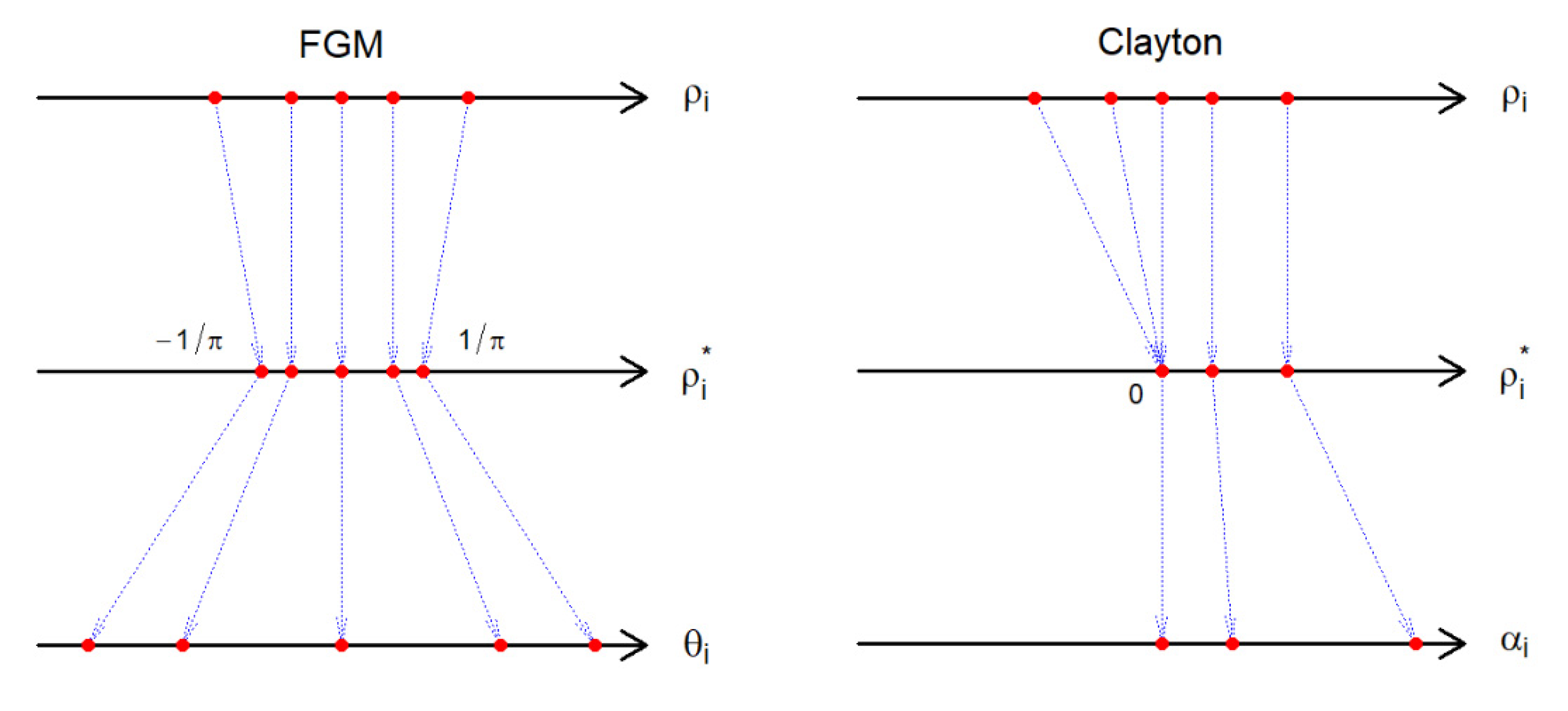
. Thus, the copula parameter is identified by , as long as . If , we suggest or , using , where . Hence, can still be identified by . This boundary enforcement is illustrated in Figure 1. Example 3. (The Clayton copula): Under the Clayton copula, the model in Equation (2)
becomesfor . The correlation function does not have a closed-form, and is written asIt is known that and . In addition, if then for all [
45]
. Then, we conclude that the range of the correlation is . Thus, one can identify by solving numerically if . If , we suggest the independence model (
Figure 1)
Example 4. (The Gumbel copula): Under the Gumbel copula, the model in Equation (2)
becomesfor . Similar to the Clayton copula, the correlation function does not have a closed-form, and is not displayed here. It is known that and . If , we suggest the independence model as in the Clayton copula. Example 5. (The Frank copula): Under the Frank copula, the model in Equation (2)
becomesfor . Again, the correlation function does not have a closed-form, and is not displayed here. It is known that and . Thus, the Frank copula parameter does not require boundary correction. 3.2. Statistical Inference Methods
This subsection develops statistical inference methods under the proposed model.
We propose the MLE for
under the general copula model (Definition 1) in Equation (2). Suppose that the copula density
exists. Then, the joint density of
is
where
and
is the density of
. Given the samples, the log-likelihood function is
The MLE of the common mean vector is defined as
where
is a real line. The MLE does not have a closed-form expression except for the normal copula. Thus, the MLE can also be obtained by the Newton–Raphson algorithm or some software functions (e.g., the R functions
optim or
nlm). One may also apply our R package
CommonMean.Copula [
26], which will be explained in
Section 6.
3.3. Information Matrix
For the MLE to be well-behaved, it is necessary to show that the (Fisher) information matrix exists and is non-singular. In other words, the MLE, without verifying these conditions, may have some problems, e.g., the non-existence, inconsistency, or inefficiency of the MLE. Furthermore, the information matrix describes how a copula influences the MLE.
We define the
information matrix
for
as
The following theorem gives the formula of the information matrix.
Lemma 1. If,, andexist in, for each, the following equalities hold Many copulas have
,
, and
in
, such as the normal, FGM, and Clayton copulas (
Appendix A.2.). The following theorem gives the formula of the information matrix.
Theorem 1. Under the copula-based model (Definition 1), the information matrix does not depend on. Furthermore, if,, andexist in, it can be decomposed into the sum of the information matrix for the independent model and the additional information by the copula,where Theorem 1 can be proved by straightforward calculations as Lemma 1 (
Appendix A.1.). Theorem 1 helps us interpret the role of the copula
on the information matrix.
Theorem 2. The determinant ofcan be expressed asIn addition,andis positive definite. Proof of Theorem 2. The expression of
is obtained by straightforward calculations. Clearly, we have
. Then, by the Cauchy-Schwarz inequality,
Furthermore, by the arithmetic-geometric mean inequality, we have
Then we obtain . Since , both the upper left and determinants of are positive. Thus, is positive definite. □
Based on Theorem 1, one can derive the information matrix for parametric copulas. Below, we show examples of the normal, FGM, and Clayton copulas.
Example 6. (The normal copula): Under the normal copulaThen, by Theorem 1, the information matrix in Equation (3)
becomes and its determinant is . Clearly, is positive definite. Example 7. (The FGM copula): Under the FGM copulaThen, by Theorem 1, the information matrix in Equation (3)
becomes By Theorem 2, its determinant is This result agrees with [
3]
who considered the FGM model. Example 8. (The Clayton copula): Under the Clayton copulaThen, by Theorems 1 and 2, we obtainandaccordingly. 4. Asymptotic Theory
To assess the sampling variability of , its asymptotic distribution is presented in this section.
A technical burden comes from the fact that our samples
,
are independent and
non-identically distributed (i.n.i.d.) owing to heterogeneous variances (
). The existence of the asymptotic distribution requires the stabilization of the information matrix [
3,
46,
47] in large samples. For the asymptotic variance of
, to be defined, we assume the existence of a
positive definite matrix
. We further assume that the copula’s derivatives
,
,
, and
exist in
. With these conditions and many other technical conditions given in [
48], we establish the consistency and asymptotic normality of
:
Theorem 3. Under the copula model (Definition 1), if some regularity conditions hold, then
- (a)
Existence and consistency: With probability tending to one, there exists the MLEsuch that, as;
- (b)
Asymptotic normality:, as.
The proof of Theorem 3 and the required regularity conditions are given in the Ph.D dissertation of [
48]. The proof approximates
by the sum of independent random variables, and then applies the weak law of large numbers for i.n.i.d. random variables from Theorem 1.14 in [
49] and the Lindeberg–Feller multivariate central limit theorem from Proposition 2.27 in [
50]. The proof is fairly technical, but similar to those of Theorem 6.5.1 in [
51], Theorem 1 in [
47], and Theorem 5.1 in [
3].
5. SE and Confidence Sets
As
Section 4 has established the asymptotic theory to evaluate the variability of the proposed MLE, we can derive the SE, confidence interval (CI), and confidence ellipse (CE).
Let
be a differentiable function, and
be the parameter of interest. For instance,
and
can be considered. The SE of
is
This formula is based on the delta method and the large sample approximation
The 95% CI for is .
Moreover, based on Theorem 3, we construct a 95% CE for
:
where
is be the 95% point of the
-distribution with two degrees of freedom.
6. R Package
We implement the proposed methods in an R package
CommonMean.Copula [
26]. R users can easily compute the MLE with its SE and 95% CI under the FGM, Clayton, Gumbel, Frank, and normal copulas. In this package, the log-likelihood is maximized by the R
optim function, where the initial values are set as the univariate estimators
For illustration, we fitted the Clayton copula by the following R codes:
- some outputs are omitted for brevity –
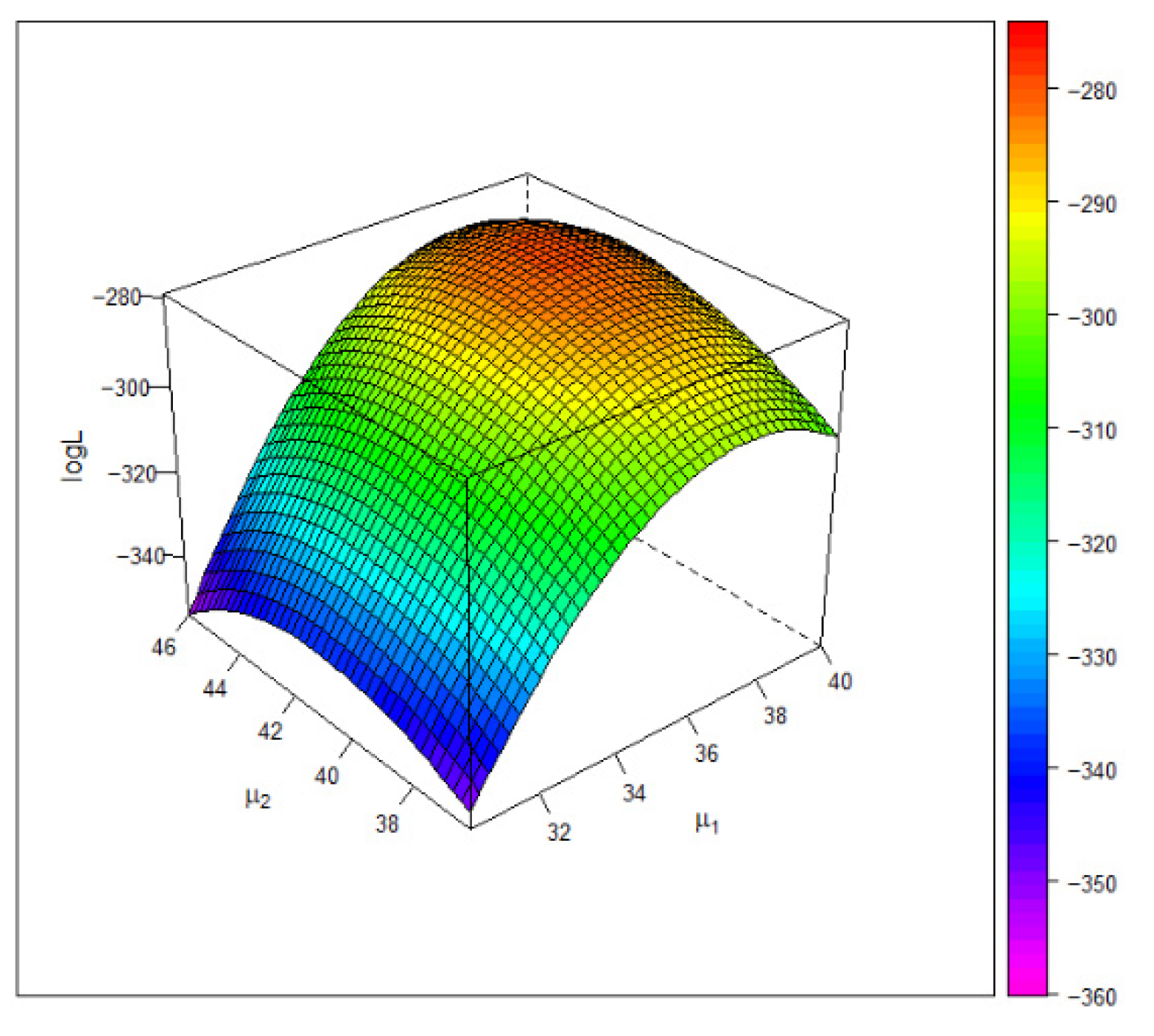
Here, $CommonMean1 shows , , and the 95% CI (33.089, 34.812); $CommonMean2 is similar. $V shows the covariance matrix . $‘Log-likelihood values’ shows . One can fit other copulas by changing “Clayton” to “FGM”, “Gumbel”, “Frank”, or “normal”.
7. Simulation Studies
We conducted Monte Carlo simulations to examine the accuracy of the proposed methods. We report the results for the Clayton copula; more results are available from [
48].
We generated
,
, under the Clayton copula with
,
, or
, leading to
,
, or
, respectively. In all three cases, we have
. Without loss of generality, we set
. To set
and
, we followed the simulation setting of [
52]. That is,
, restricted in the interval
. This setting leads to
. Based on the generated data, we computed
,
, and
, and their SEs and 95% CIs (CEs) by using the R function
CommonMean.Copula (
Section 6). We then evaluated the coverage probability (CP) of the 95% CI (CE) to see how the confidence set can cover the true value. We consider a small sample size
and a large sample size
. Our simulations are based on 1000 repetitions.
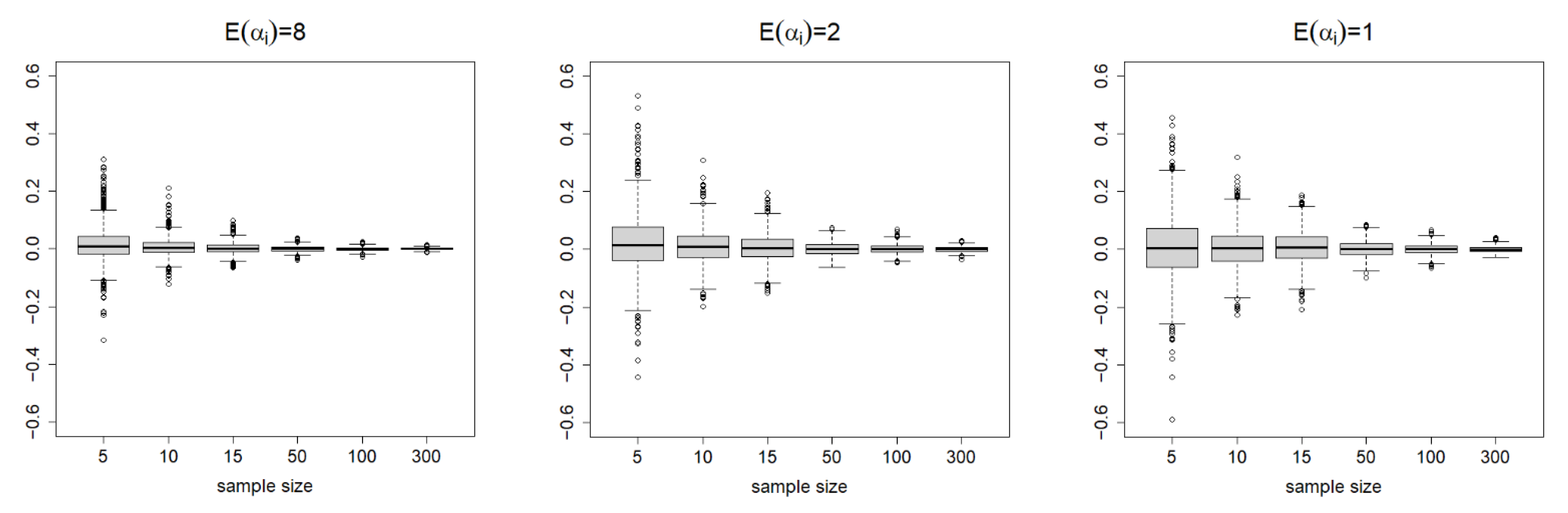
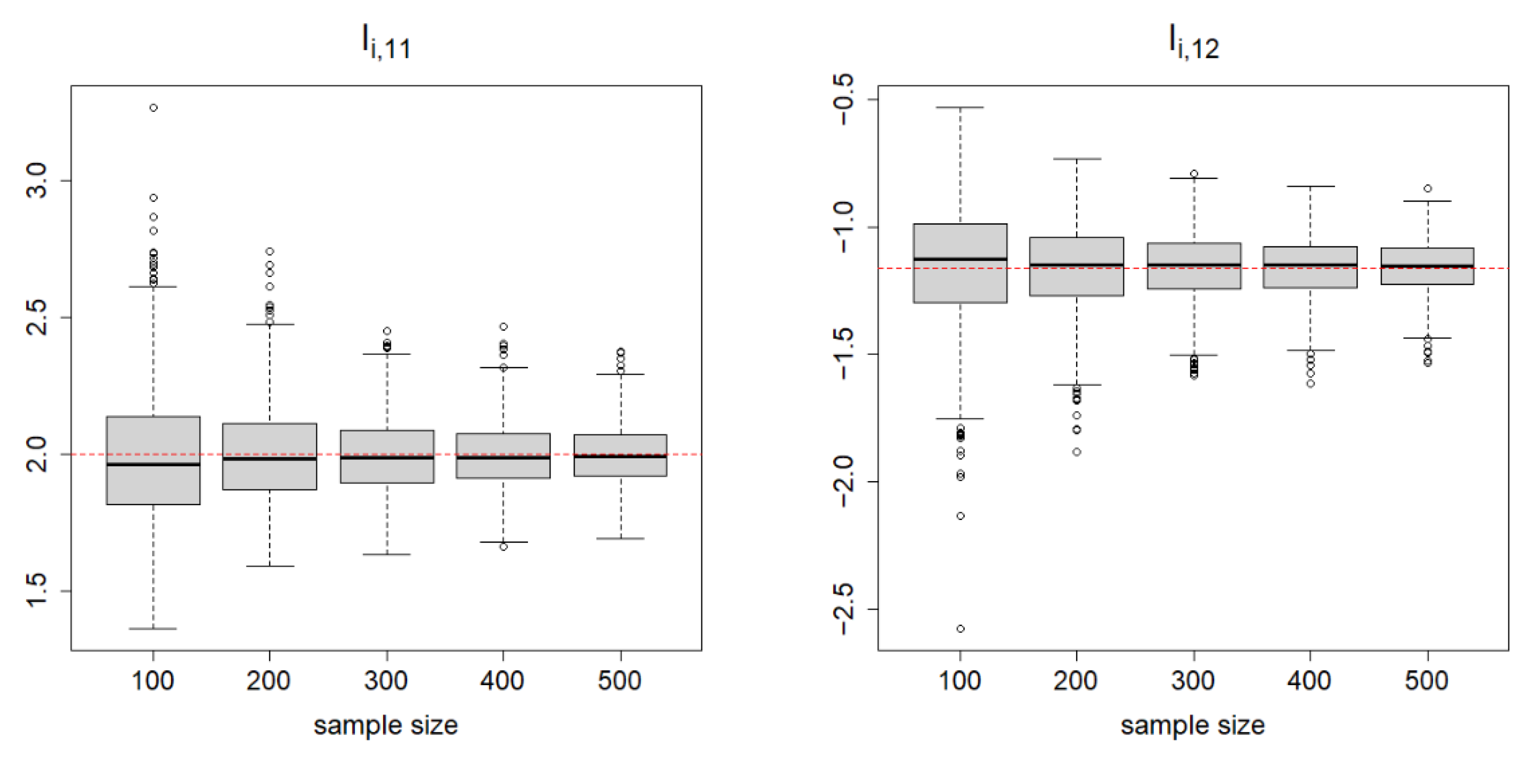
Table 1 summarizes the results. For
and
, the SDs of the estimates decrease when
increases from
to
. We report the boxplots summarizing the 1000 repetitions for
in
Figure 2. This clearly visualizes how the variability of the estimates vanishes as the sample sizes increase.
Table 1 also shows that the SDs are close to the average SEs, except for
(due to the very small samples). Consequently, the CPs are close enough to the nominal level of 0.95, especially when sample sizes are large, which is consistent with our asymptotic theories. For
, the CPs of the 95% CEs are also reasonably close to the nominal level. In summary, the proposed estimators and the asymptotic theory work fairly well in finite samples.
9. Extension to Non-Normal Models
So far, we have considered a common mean model under the marginal normality. This section explains how the proposed methods can be extended to non-normal models. For this reason, we specifically consider a common mean model under the marginal exponential distributions.
Thus, the common mean vector is
We consider the Clayton copula to specify the bivariate distribution because it has simple derivatives with respect to the copula parameter [
54]. Therefore, we propose a bivariate common mean Clayton copula model with exponential margins as follows:
where
is known for
. Note that copula
is a survival copula for (
as the usual way to model a survival function [
22]. Using similar arguments to [
55], the information matrix with respect to
can be decomposed as
where
See
Appendix A.3. for detailed derivations. The expression of
is an extension of Theorem 3 to the exponential model. With the information matrix, the properties of the MLE and the asymptotic theory are similar to the normal models.
We conducted Monte Carlo simulations to examine the correctness of Equation (5) by comparing it with their empirical version. We set
and
for all
. We generated data
from the model in Equation (4) and computed the empirical versions of
and
as
The formulas for the derivatives of the log-density are found in Equations (A1) and (A2) in
Appendix A.3. Our simulations were based on 1000 repetitions with
.
Figure 7 depicts the simulation results based on 1000 repetitions. It clearly shows that the empirical versions are scattered around the theoretical values of
and
. The variability of the empirical versions vanishes as
increases. The simulation results assert the correctness of Equation (5).
10. Conclusions
At present, copula models are very popular in all areas of science. Bivariate meta-analyses are among those research areas that require sophisticated copula-based methods and theories. Nonetheless, there are only a few studies on copula-based bivariate meta-analysis from a methodological/theoretical perspective. This article fully develops the methodologies and theories of the copula-based bivariate meta-analysis, specifically for estimating the common mean vector. These developments will provide solid methodological/theoretical bases that are not available to date.
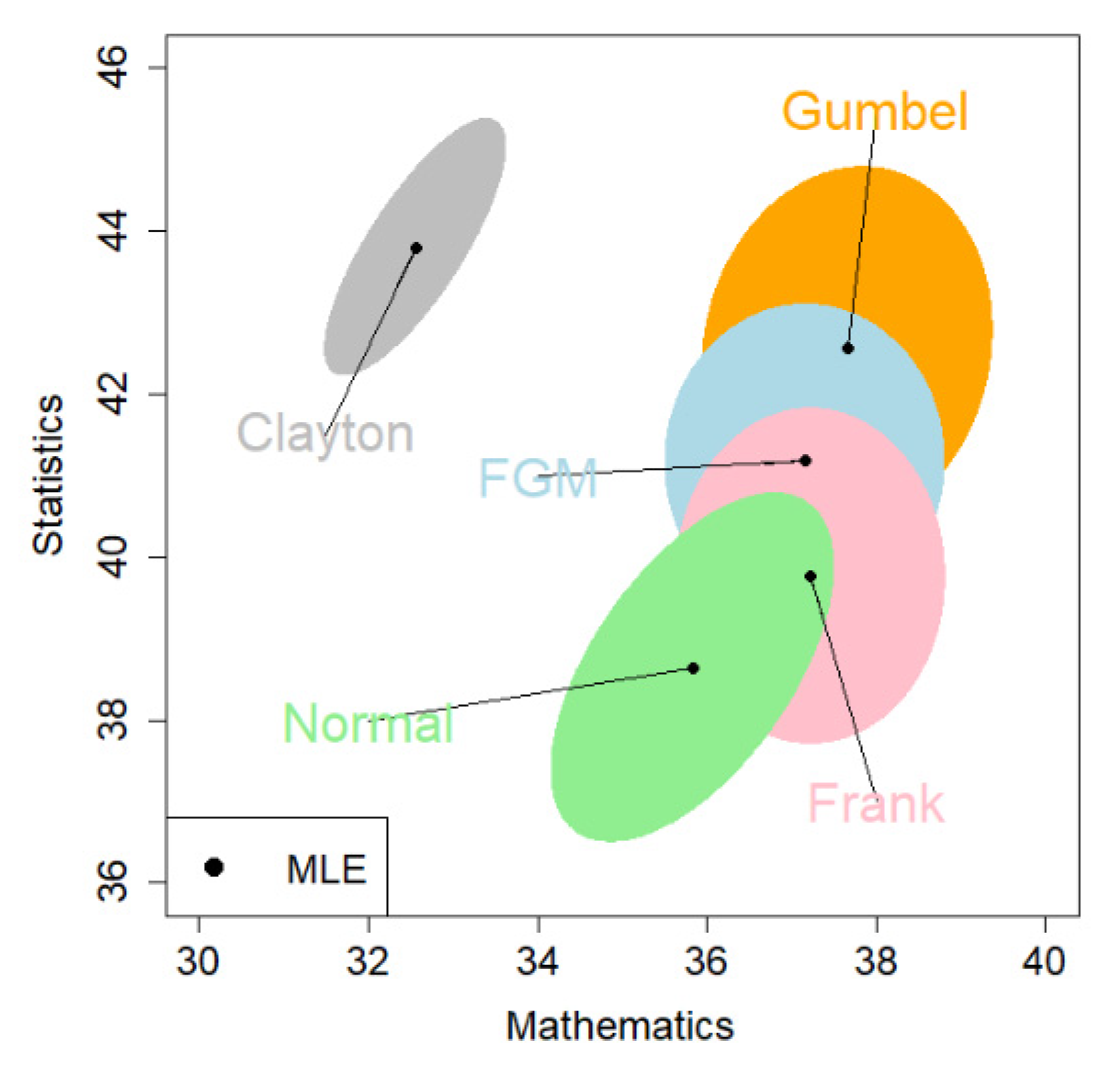
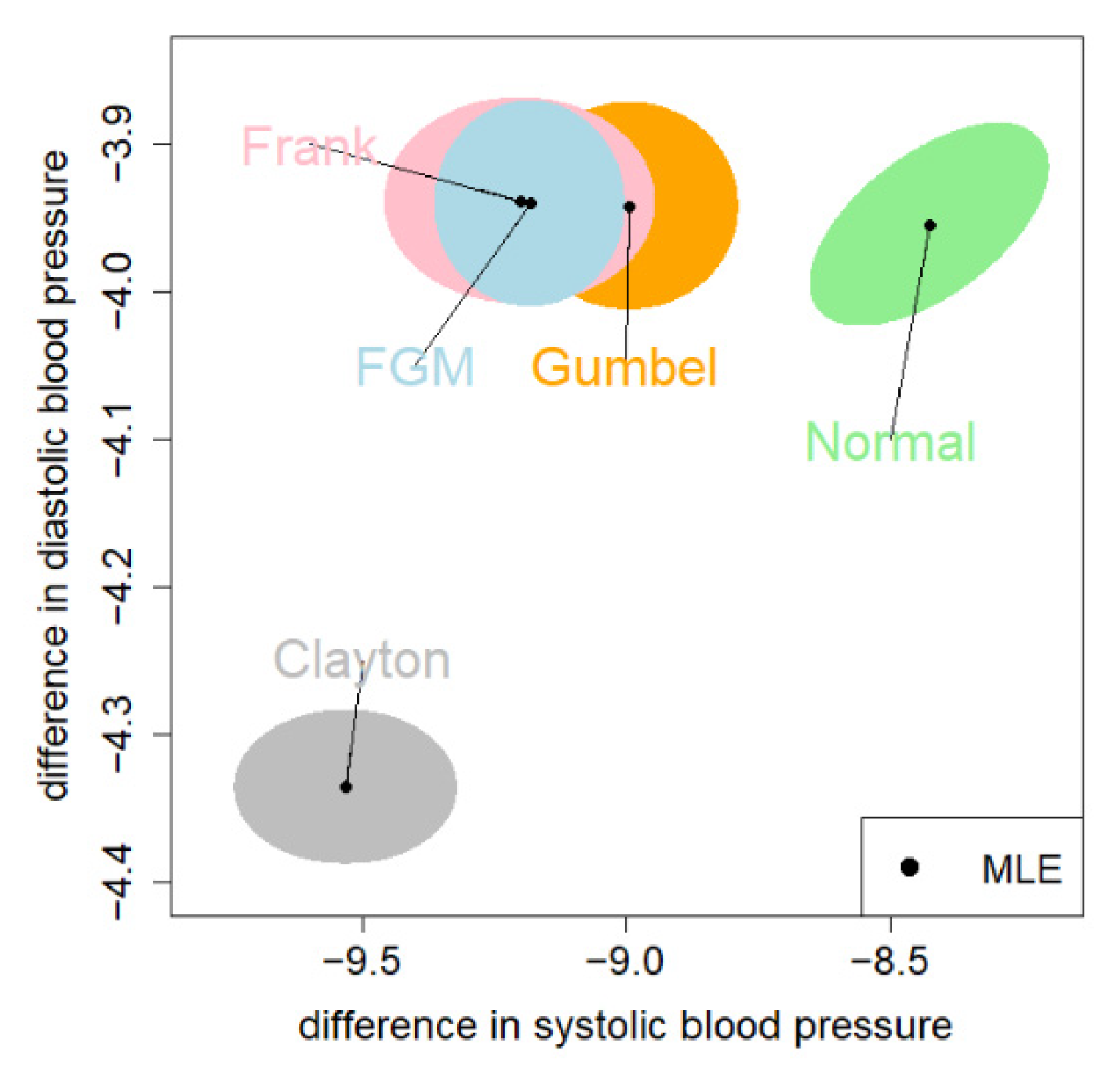
In this article, we emphasize the flexibility of the proposed copula models that allow for a variety of dependence structures. In the two real data examples, we employed the log-likelihood value as a criterion for model selection (
Section 8). Even if the best copula is selected, it still raises the issue of goodness-of-fit, which is difficult to assess under the meta-analysis setting. The classical methods, such as Kolmogorov–Smirnov or Cramér–von Mises type statistics, cannot be directly applied to the non-identically distributed samples for which the empirical distribution function is difficult to interpret. Therefore, the development of goodness-of-fit tests is a possible research direction.
The fundamental assumption made in the proposed model is the common mean model, with known within-study correlations. The common mean assumption, although convenient for summarizing the data for a small number of studies [
56], may not always hold in real meta-analyses [
6]. Therefore, the extension of the proposed estimator to random means (random-effects models) or ordered means [
57,
58] is an important direction for future research. To model the random effects, we need another bivariate copula. The estimation problem for these hierarchical copula-based models is beyond the scope of the paper. Nonetheless, the results presented in this paper serve as fundamental knowledge before the exploration of more advanced models.


