In this section, we present three methods to compute the nonlinearity of a B.f. f. The first exploits Gröbner basis algorithms over the binary field, and is somehow inefficient, but beside the nonlinearity, also returns all affine functions of a given distance from f. The second methods is more efficient and uses Gröbner basis algorithms over the rational or a prime field. Finally, the third method, the most efficient, is based on a butterfly structure similar to a fast Fourier transform.
4.1. Gröebner Bases over the Biniary Field
In this section, we show how to use Theorem 1 to compute the nonlinearity of a given B.f. . We want to define an ideal such that a point in its variety corresponds to an affine function with distance at most from f.
Let
A be the variable set
. We denote by
the following polynomial:
According to Lemma 1, determining the nonlinearity of
is the same as finding the minimum weight of the vectors in the set
. We can consider the evaluation vector of the polynomial
as follows:
Example 2. Let be a general affine function in . Then . We consider vectors in ordered as follows (note that, in all the examples, we first list the vectors from smaller to higher Hamming weight. Among vectors of the same weight, we list first those having a smaller integer representation, with least significant bit on the right):Thus, we have that the evaluation vector of is Definition 9. We denote by the ideal in : Remark 1. As , is zero-dimensional and radical ([38]). Lemma 2. For the following statements are equivalent:
- 1.
,
- 2.
,
- 3.
.
(1)⇒(2). Let and . We have that for all . Thus, and, thanks to Theorem 1, , i.e., .
(2)⇒(1). It can be proved by reversing the above argument. □
From Lemma 2 we immediately have the following theorem.
Theorem 2. Let . The nonlinearity is the minimum t such that .
From this theorem we can derive an algorithm to compute the nonlinearity for a function , by computing any Gröbner basis of .
Remark 2. If f is not affine, we can start our check from .
Example 3. Let be the Boolean function: We want to compute and clearly f is not affine. We compute vector and we take a general affine function (as in Example 2), so that , Thus, . The ideal is the ideal generated by We compute any Gröbner basis of this ideal and we obtain that it is trivial, so and . Now we have to compute a Gröbner basis for . We obtain, using degrevlex (graded reverse lexicographic order, also known as grevlex, or degrevlex for degree reverse lexicographic order, compares the total degree first, then uses a reverse lexicographic order as tie-breaker, but it reverses the outcome of the lexicographic comparison so that lexicographically larger monomials of the same degree are considered to be degrevlex smaller). Ordering with , that . Thus, by Theorem 2. By inspecting , we also obtain all affine functions having distance 2 from f:
Example 4. Let be the Boolean function As it is obvious that f is not affine, we start from the ideal . The Gröbner basis of is trivial with respect to any monomial order for . For , we obtain the Gröbner basis with respect to the degrevlex order with : Then , that is, there is only one affine function α that has distance equal to 4 from f: .
4.2. Gröebner Bases over the Rational Field
Here we present an algorithm to compute the nonlinearity of a B.f. using Gröbner bases over
rather than over
, which turns out to be much faster than Algorithm 1. The same algorithm can be slightly modified to work over the field
, where
p is a prime. The complexity of these algorithms will be analyzed in
Section 5.
| Algorithm 1. Basic algorithm to compute the nonlinearity of a B.f. using Gröbner basis over . |
| Input: a B.f. f |
| Output: the nonlinearity of f |
| 1: |
| 2: while do |
| 3: |
| 4: end while |
| 5: return |
As we have seen in
Section 4.1, the nonlinearity of a B.f. can be computed using Gröbner bases over
. It is sufficient to find the minimum
j such that the variety of the ideal
is not empty. Recall that
This method becomes impractical even for small values of n, since monomials have to be evaluated. A first slight improvement could be achieved by adding to the ideal one monomial evaluation at a time and check if 1 has appeared in the Gröbner basis. Even this way, the algorithm remains very slow.
For each
, let us denote:
the B.f. where as usual
are the
variables representing the coefficient of a generic affine function. In this case we have that:
Note that the polynomials
are affine polynomials. We also denote by
the NNF of each
(obtained as in [
33], Theorem 1).
Definition 10. We call the integer nonlinearity polynomial (or simply the nonlinearity polynomial) of the B.f. f. For any we define the ideal as follows: Note that the evaluation vector represents all the distances of f from all possible affine functions (in n variables).
Theorem 3. The variety of the ideal is non-empty if and only if the B.f. f has distance t from an affine function. In particular, , where t is the minimum positive integer such that .
Proof. Note that and so Therefore, if and only if such that . Let such that . By definition we have and Hence and our claim follows directly. □
To compute the nonlinearity of
f we can use Algorithm 2 over the rational field (
), with input
f.
| Algorithm 2. To compute the nonlinearity of the B.f. f using Gröbner basis over a field . |
| Input:f |
| Output: nonlinearity of f |
| 1: Compute |
| 2: |
| 3: while do |
| 4: |
| 5: end while |
| 6: return j |
4.4. Properties of the Nonlinearity Polynomial
From now on, with abuse of notation, we sometimes consider 0 and 1 as elements of and other times as elements of . We have the following simple lemma:
Lemma 3. Given where the sum on the right is in . It is easy to show that . We give a theorem to compute the coefficients of the nonlinearity polynomial.
Theorem 4. Let , , and be such that . Then the coefficients of can be computed as: Proof. The nonlinearity polynomial is the integer sum of the
numerical normal forms of the affine polynomials
, each identified by the vector
, i.e.,:
which is a polynomial in
. The NNF of
is a polynomial with
terms, i.e.,:
for some
, and by Proposition 1
Let us prove Equation (
3). When
we have
Let us prove Equation (4). Suppose
. Now the coefficient
of the monomial
of the nonlinearity polynomial is such that:
We claim that each
u such that
yields a zero term in the summation. If
then
s.t.
, i.e.,
. We show now that
s.t.
s.t.
and
It is sufficient to choose
and
for all
. Clearly
and
since
. By direct substitution we obtain
Thanks to (
6) we can continue from (
5) and get
where we used
.
Now we consider
fixed, and
. There are exactly
vectors
a such that
, i.e.,:
Now we want to study the internal summation in (
7). If
then
we have
. Otherwise, if
we can consider the following set of indices
, which has size
. Since
and
then
by transitivity. For all
we have
, and then
. Thus, for any
we have
and each of the two cases happens for exactly one half of the vectors
. Clearly the two halves are disjointed. This yields, from (
5) and (
7), the following chain of equalities:
which proves the theorem. □
In particular we have:
Corollary 1. Let and the nonlinearity polynomial Furthermore, we have: Corollary 1 shows that it is sufficient to store half of the coefficients of , precisely the coefficients of the monomials where does not appear.
Corollary 2. Each coefficient c of the nonlinearity polynomial is such that .
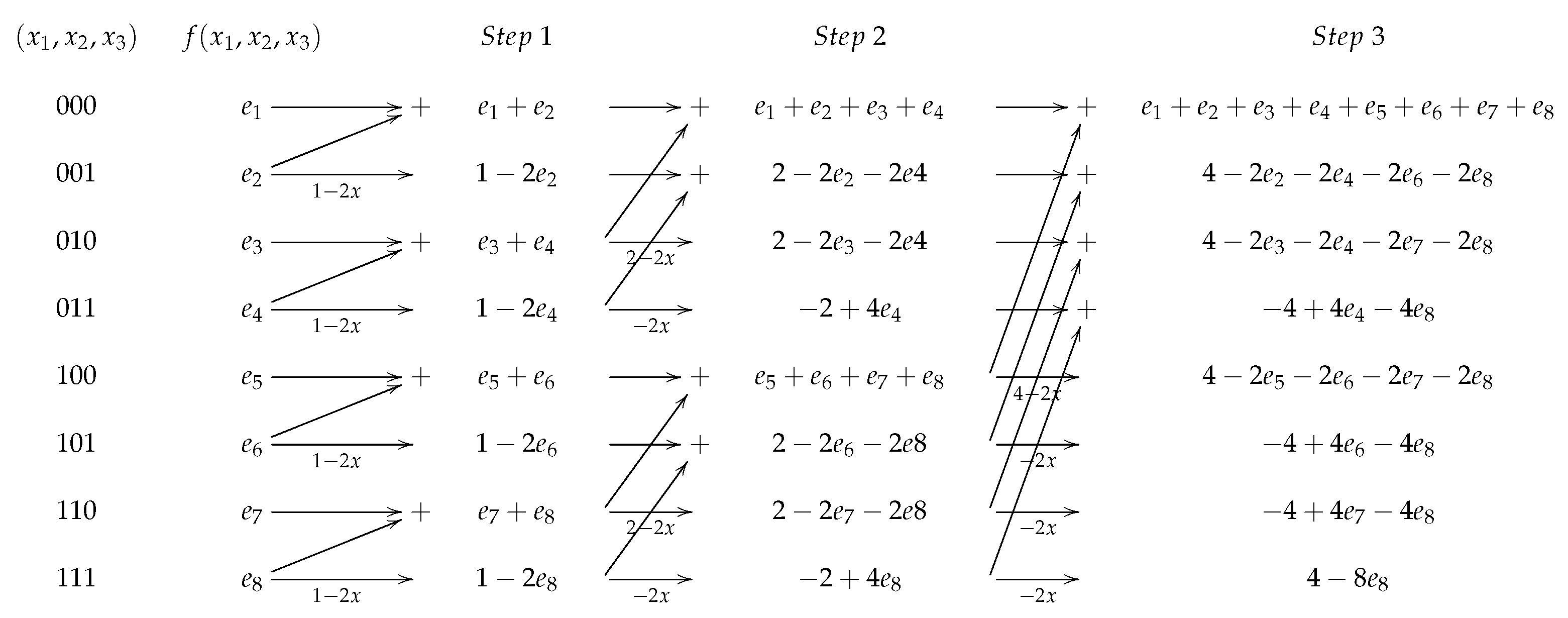
Corollary 3. Given the nonlinearity polynomial of f asthen the nonlinearity polynomial of is related to that of f by the following rule: A scheme that shows how to derive the coefficients of the nonlinearity polynomial in the case
can be seen in
Table 1 and
Table 2.


