Higgs Boson-Induced Reheating and Dark Matter Production

Abstract

We discuss a perturbative and non-instantaneous reheating model, adopting a generic post-inflationary scenario with an equation of state w. In particular, we explore the Higgs boson-induced reheating, assuming that it is achieved through a cubic inflaton-Higgs coupling ${\varphi \left|\mathcal{H}\right|}^2$. In the presence of such coupling, the Higgs doublet acquires a $\varphi$-dependent mass and a non-trivial vacuum–expectation–value that oscillates in time and breaks the Standard Model gauge symmetry. Furthermore, we demonstrate that the non-standard cosmologies and the inflaton-induced mass of the Higgs field modify the radiation production during the reheating period.This, in turn, affects the evolution of a thermal bath temperature, which has remarkable consequences for the ultraviolet freeze-in dark matter production.

1. Introduction

The standard model of cosmology is based on the assumption that the Universe at its very beginning underwent a phase of rapid, exponential expansion, driven by some dynamical field—the so-called inflaton $\varphi$ [1,2]. Although we still do not have any direct evidence for this period, the inflationary paradigm is nowadays well-established and consistent with all observations [3]. On the other hand, measurements of the relative abundances of light elements indicate that shortly after the end of inflation, the Universe was filled with a hot plasma of relativistic particles [4]. Because the rapid expansion diluted all matter particles and left the early Universe cold and almost empty, any successful model of a primordial Universe should account for how the Universe transitioned from an inflationary to a radiation-dominated (RD) epoch. The reheating mechanism has been introduced to explain the transfer of energy initially stored in coherent oscillations of the inflaton field to other relativistic degrees of freedom and render the Universe hot [5,6,7,8]. This can be achieved through some coupling between the inflaton and the visible sector.

Typically, the relevance of the reheating dynamics is ignored with a trio of simplifying assumptions: standard cosmology, instantaneous reheating, and instantaneous thermalization of the inflaton’s decay products. In this work, we maintain the last assumption and relax the first two. Namely, we consider the non-standard scenario of the early Universe, assuming that it features a phase of non-standard expansion that depends on the generic equation-of-state w, which in turn, can be related to the form of the inflaton potential [9,10,11]. Moreover, we assume that the leading interaction of the inflaton with the Standard Model (SM) sector is through the Higgs portal ${\varphi \left|\mathcal{H}\right|}^2$. Not only does this operator describe the perturbative decay of the $\varphi$ field into the pairs of the SM Higgs particles, but it also generates a $\varphi$-dependent mass and a vacuum–expectation–value (vev) of the Higgs doublet [12]. It turns out that in this case, the inflaton decay rate, ${\Gamma }_{\varphi }$ becomes a function of time [12]. Such time-dependence of ${\Gamma }_{\varphi }$ can be generated by the inflaton-induced mass of the Higgs doublet [12], and the non-standard form of the inflaton potential [11,12]. It turns out that it has non-trivial consequences for the dynamics of the reheating period in both cases. In particular, the time-dependence of the inflaton decay rate can affect the evolution of the SM radiation energy density, and thus a thermal bath temperature during reheating [12]. In contrast, the non-zero mass of the inflaton’s decay products is a source of a kinematical suppression that leads, e.g., to a decrease in the reheating temperature.

The suppression of the radiation production and the modified evolution of the thermal bath temperature may have non-trivial consequences for dark matter (DM) production. For instance, in the ultraviolet (UV) freeze-in mechanism the production of DM particles occurs mainly at the highest possible temperatures and thus can be potentially sensitive to the details of reheating [13]. As an illustration of this effect, we consider a simple DM model, assuming that the dark sector consists of spin-1, massive particles that interact only gravitationally; for a review see [14,15,16,17].

The paper is structured as follows: In the first part, we provide a brief introduction to the primordial Universe, focusing on the $\alpha$-attractor T-model of inflation [18,19]. In particular, we present the analytical approximations and full numerical solutions to the equation of motion for the inflaton during the reheating phase and derive the relation between the averaged equation-of-state parameter w and the parameters of the inflaton potential. In Section 3 we investigate the production of SM radiation energy density, considering the Higgs portal interaction between the inflaton and the SM Higgs doublet. There we present numerical solutions to the set of two coupled Boltzmann equations and discuss the role of the time-dependent inflaton decay width for the evolution of the inflaton and the SM radiation energy densities. In Section 4 we present the consequences of the non-standard reheating dynamics for the dark sector in the context of a UV freeze-in DM production. In Section 5 we summarize our work.

2. Inflaton Dynamics

In this work, we assume that the accelerated expansion of the early Universe is driven by a single real-scalar field, $\varphi$, that is minimally coupled to gravity. The action for our inflationary model is

$$S=\int d^{4}x\sqrt{-g}\left\{\frac{M_{\mathrm{Pl}}^2}{2}R+\frac{1}{2}{\partial }_{\mu }\varphi {\partial }^{\mu }\varphi -V\left(\varphi \right)\right\},$$

(1)

where $M_{\mathrm{Pl}}\simeq 2.4\times {10}^{18}\mathrm{GeV}$ is the reduced Planck mass, whereas R and g denote the Ricci scalar for a background metric $g_{\mu \nu }$ and its determinant, respectively. For concreteness, we consider the $\alpha$-attractor T-model of inflation [18,19], such that the inflaton potential has a tangent-hyperbolic form,

$$V\left(\varphi \right)={\Lambda }^4{tanh}^{2n}\left(\frac{\left|\varphi \right|}{M}\right).$$

(2)

Above, $\Lambda$ determines the scale of inflation, while n and $M\equiv \sqrt{6\alpha }{M}_{\mathrm{Pl}}$ are two parameters of the model. The amplitude of the scalar power spectrum measured by the Planck satellite [20] (${\Delta }_s^2\left(k_{★}\right)=2.1\times {10}^{-9}$, with $k_{★}=0.05{\mathrm{Mpc}}^{-1}$) and the current upper bound on the tensor-to-scalar ratio ($r<0.06$) set the following upper limit on $\Lambda \lesssim 1.6\times {10}^{16}\mathrm{GeV}$ and $M\lesssim 10M_{\mathrm{Pl}}$. In what follows, we fix these two parameters to $M=M_{\mathrm{Pl}}$ ($\alpha =1/6$) and $\Lambda ={10}^{16}\mathrm{GeV}$, and consider two values of n, i.e., $n=1$ and $n=3/2$. Let us also note that Equation (1) neglects all possible interactions with other sectors, which is a reasonable assumption during inflation and early stages of reheating.

For the FLRW metric with the scale factor $a\left(t\right)$, such that $\sqrt{-g}=a^3$, one obtains from (1) the Euler–Lagrange equation for the $\varphi$ field,

$$\ddot{\varphi }+3H\dot{\varphi }+V^{\prime }\left(\varphi \right)=0,$$

(3)

where the prime is derivative of the potential with respect to $\varphi$, while the overdot denotes derivative with respect to the cosmic time t. The evolution of the Hubble rate, $H\equiv \dot{a}/a$, is captured by the Friedmann equation, $H^2={\rho }_{\varphi }/\left(3M_{\mathrm{Pl}}^2\right)$. Note that in the above equation we have neglected the spatial derivatives of the $\varphi$ field, treating $\varphi$ as a homogeneous scalar field, i.e., $\varphi =\varphi \left(t\right)$. Its energy density and the pressure are simply

$$\begin{array}{cccc}\hfill {\rho }_{\varphi }& =\frac{1}{2}{\dot{\varphi }}^2+V\left(\varphi \right),\hfill & \hfill p_{\varphi }& =\frac{1}{2}{\dot{\varphi }}^2-V\left(\varphi \right).\hfill \end{array}$$

(4)

Let us now discuss two types of solutions to Equation (3), starting from the inflationary one. First of all, we should note that for large field values, i.e., $\left|\varphi \right|\gg M$, the inflaton potential (2) has a plateau: $V\left(\varphi \right)\simeq {\Lambda }^4$. Moreover, during inflation we can assume that $\ddot{\varphi }\simeq 0$ and $\frac{1}{2}\dot{\varphi }\ll V\left(\varphi \right)$. These assumptions allow us to find the so-called slow-roll solutions: ${\varphi }_I\left(t\right)\sim const.$ and $H_I\simeq {\Lambda }^2/\left(\sqrt{3}{M}_{\mathrm{Pl}}\right)$. Inflation ends when $\ddot{a}=0$, which corresponds to ${ϵ}_V\equiv 1/2{(M_{\mathrm{Pl}}{V}_{,\varphi }\left(\varphi \right)/V\left(\varphi \right))}^2=1$. Shortly after this moment $\varphi$ drops below M and $V\left(\varphi \right)$ can be well approximated by the following monomial form,

$$\begin{array}{ccc}\hfill V_o\left(\varphi \right)& \simeq {\Lambda }^4{\left(\frac{\left|\varphi \right|}{M}\right)}^{2n},\hfill & \hfill \mathrm{for}t>t_e,\end{array}$$

(5)

where $t_e$ denotes the cosmic time at the end of inflation.

The $\varphi$ field starts to oscillate around the minimum of its potential, and the generic solution to the inflaton equation of motion (3) can be written as a product of two functions [7,11]

$$\begin{array}{ccc}\hfill {\varphi }_o\left(t\right)& =\phi \left(t\right)\mathcal{P}\left(t\right),\hfill & \hfill \mathrm{for}t>t_e,\end{array}$$

(6)

with $\phi$ being the slowly varying envelope function, defined by the condition $V_o\left(\phi \right)=\langle {\rho }_{\varphi }\rangle$. Here $\langle {\rho }_{\varphi }\rangle$ stands for the time-averaged inflaton energy density,

$$\langle {\rho }_{\varphi }\rangle \left(t_0\right)\equiv \frac{1}{T\left(t_0\right)}{\int }_{t_0}^{t_0+T\left(t_0\right)}dt{\rho }_{\varphi }\left(t\right),$$

(7)

where $T\left(t_0\right)$ is the period of the oscillations at $t=t_0$. Above, $\mathcal{P}\left(t\right)$ denotes a fast-oscillating quasi-periodic function. One can show that $\phi$ has to satisfy the following equation

$$\dot{\phi }\left(t\right)=-\frac{3}{n+1}H\phi \left(t\right),$$

(8)

where we have used relation between the averaged equation-of-state paramater w and n:

$$w\equiv \frac{\langle p_{\varphi }\rangle }{\langle {\rho }_{\varphi }\rangle }=\frac{n-1}{n+1},$$

(9)

which is valid during the oscillatory phase for the inflaton potential of the form (6).

The solution to the envelope function $\phi \left(a\right)$ is given by

$$\phi \left(a\right)=\phi \left(a_e\right){\left(\frac{a_e}{a}\right)}^{\frac{3}{1+n}},$$

(10)

where $\phi \left(a_e\right)=M/2ArcSinh\left(2n/\sqrt{3\alpha }\right)$ denotes the initial value of the $\phi$ function. One can show that the fast-oscillating function $\mathcal{P}$ can be written in terms of the inverse of the regularized incomplete beta function:

$$\begin{array}{ccc}\hfill \mathcal{P}\left(a\right)& ={\left[I_z^{-1}\left(\frac{1}{2n},\frac{1}{2}\right)\right]}^{\frac{1}{2n}},\hfill & \hfill z=1-\frac{4}{\mathcal{T}}\frac{1+n}{3n}\frac{\sqrt{3}{M}_{\mathrm{Pl}}}{{\Lambda }^2}{\left(\frac{\phi \left(a_e\right)}{M}\right)}^{-n}\left[{\left(\frac{a}{a_e}\right)}^{\frac{3n}{1+n}}-1\right],\end{array}$$

(11)

where the period of oscilation $\mathcal{T}$ is

$$\begin{array}{cccc}\hfill \mathcal{T}& =\frac{\sqrt{16\pi n(2n-1)}}{m_{\varphi }\left(t\right)}\frac{\Gamma \left(1+\frac{1}{2n}\right)}{\Gamma \left(\frac{1}{2}+\frac{1}{2n}\right)},\hfill & \hfill m_{\varphi }& =\sqrt{2n(2n-1)}\frac{{\Lambda }^2}{M}{\left(\frac{{\rho }_{\varphi }}{{\Lambda }^4}\right)}^{\frac{n-1}{2n}},\hfill \end{array}$$

(12)

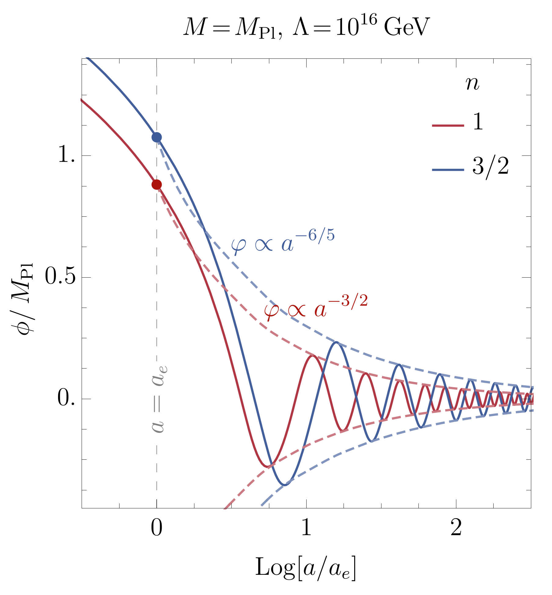
with $m_{\varphi }^2\equiv \frac{{\partial }^{2}V\left(\varphi \right)}{\partial {\varphi }^2}{|}_{\varphi =\phi }$ being an effective mass of the inflaton field. Note that for the quadratic potential ($n=1$), $m_{\varphi }=\sqrt{2}{\Lambda }^2/M$ and thus $\mathcal{T}=2\pi /m_{\varphi }$ are time independent [12]. For $n=3/2$, $m_{\varphi }$ decreases with time, which implies that $\mathcal{T}$ increases. The full numerical solutions to Equation (3) for the benchmark values of model parameters are shown in Figure 1.

3. Reheating

In this work, we assume that the energy transfer between the inflaton and the SM radiation occurs through the Higgs portal,

$$\begin{array}{c}\hfill {\mathcal{L}}_{\mathrm{int}}=g_{h\varphi }{M}_{\mathrm{Pl}}\varphi {\left|\mathcal{H}\right|}^2,\end{array}$$

(13)

where $g_{h\varphi }$ denotes a positive dimensionless coupling constant. Not only does the above operator describe the “decay” of the inflaton field, but it also generates $\varphi$-dependent mass of the SM Higgs field [12]. Requiring that an amplitude for the Higgs scattering in a background of the inflaton field with its single insertion is smaller than the corresponding amplitude with double insertion leads to an upper bound on the inflaton–Higgs coupling, $g_{h\varphi }\lesssim {\Lambda }^2/(M_{\mathrm{Pl}}\left|\varphi \right|)$. Furthermore, the stability of the Higgs potential implies the following lower limit, $g_{h\varphi }\gtrsim {\Lambda }^4/(M_{\mathrm{Pl}}^3\left|\varphi \right|)$, see also [21]. Inserting the upper limit on $\Lambda$, and taking $\left|\varphi \right|\simeq M$ we obtain the constraint ${10}^{-10}\lesssim g_{h\varphi }\lesssim {10}^{-5}$.

In the early Universe, the Higgs potential takes the form,

$$\begin{array}{c}\hfill V\left(\mathcal{H}\right)={\mu }_h^2{\left|\mathcal{H}\right|}^2+{\lambda }_h{\left|\mathcal{H}\right|}^4,\end{array}$$

(14)

where the mass parameter, ${\mu }_h$, is a function of the rapidly oscillating field $\varphi$:

$$\begin{array}{c}\hfill {\mu }_h^2={\mu }_h^2\left(\varphi \right)=g_{h\varphi }{M}_{\mathrm{Pl}}\varphi .\end{array}$$

(15)

Note that in the above expression, we have neglected the constant contribution to ${\mu }_h^2$ proportional to the electroweak vev, and thermal corrections proportional to $T^2$, which are, for the considered value of potential parameters, much smaller than ${\mu }_h^2\left(\varphi \right)$. The $\varphi$-dependent mass of the Higgs doublet also generates the non-trivial Higgs vev,

$$\begin{array}{cc}\hfill v_h& =\left\{\begin{array}{cc}0,\hfill & \varphi \left(t\right)>0,\hfill \\ \sqrt{\frac{|{\mu }_h^2\left(\varphi \right)|}{{\lambda }_h}},\hfill & \varphi \left(t\right)<0,\hfill \end{array}\right.\hfill \end{array}$$

(16)

which vanishes after the end of reheating. Note also that in the unbroken (symmetric) phase, i.e., $\varphi >0$, masses of the Higgs doublet components, $h_i$, are $m_{h_i}^2=\left|{\mu }_h^2\right|$, whereas in the broken phase, i.e., $\varphi <0$, the zero component of the Higgs doublet acquires a mass $m_{h_0}^2=2\left|{\mu }_h^2\right|$, and the three would-be Goldstone bosons acquire an infinite mass and disappear from the spectrum when the unitary gauge is adopted.

The dynamics of the early Universe is governed by the following set of two coupled, time-averaged, Boltzmann equations,

$$\begin{array}{cc}\hfill {\dot{\rho }}_{\varphi }+3\left(\frac{2n}{n+1}\right)H{\rho }_{\varphi }& =-\langle {\Gamma }_{\varphi }\rangle {\rho }_{\varphi },\hfill \end{array}$$

(17)

$$\begin{array}{cc}\hfill {\dot{\rho }}_{\mathcal{R}}+4H{\rho }_{\mathcal{R}}& =+\langle {\Gamma }_{\varphi }\rangle {\rho }_{\varphi },\hfill \end{array}$$

(18)

with the following initial conditions:

$$\begin{array}{ccc}\hfill {\rho }_{\varphi }\left(a_e\right)& ={\Lambda }^4|\frac{1}{2}ArcSinh\left(\frac{2n}{\sqrt{3\alpha }}\right){|}^{2n},\hfill & \hfill {\rho }_{\mathcal{R}}\left(a_e\right)=0.\end{array}$$

(19)

Let us emphasize that in the second Boltzmann Equation (18) we have assumed that the whole radiation sector is produced through the Higgs interactions and thermalizes instantaneously. Moreover, we treat the inflaton as a spatially homogeneous classical field. Within this framework, Higgs particles are created out of a vacuum in the presence of the periodically changing $\varphi$ field [22]. Consequently, $\langle {\Gamma }_{\varphi }\rangle$ should be interpreted as the time-averaged inflaton “decay” rate that parametrizes the loss of the inflaton energy density due to particle production. Assuming that $\langle {\Gamma }_{\varphi }\rangle \simeq \langle {\Gamma }_{\varphi \to hh}\rangle$ one can show that it can be calculated as,

$$\begin{array}{cc}\hfill \langle {\Gamma }_{\varphi }\rangle & =\frac{g_{h\varphi }^2}{32\pi }\sqrt{2\pi 2n(2n-1)}\frac{\Gamma \left(\frac{1}{2}+\frac{1}{2n}\right)}{\Gamma \left(1+\frac{1}{2n}\right)}\frac{M_{\mathrm{Pl}}^2}{m_{\varphi }}\sum _{i=0}^3\sum _{k=0}^{\infty }k{\left|P_k\right|}^2〈\mathrm{Re}\left[\sqrt{1-{\left(\frac{2m_{h_i}}{k\omega }\right)}^2}\right]〉,\hfill \end{array}$$

(20)

where we have decomposed the fast-oscillating function $\mathcal{P}$ into Fourier modes, i.e., $P\left(t\right)={\sum }_{k=0}^{\infty }{P}_k{e}^{-ik\omega t}$. In the above expression, $\omega =2\pi /\mathcal{T}$ denotes the frequency of the oscillations. Note that in a general case, i.e., $n\ne 1$, the inflaton decay width has two sources of time dependence: the inflaton mass $m_{\varphi }$, defined in Equation (12), and the inflaton-induced mass of the Higgs doublet. Nonetheless, as pointed out in even for the quadratic inflaton potential and $n=1$, for the non-negligible Higgs mass, $\langle {\Gamma }_{\varphi }\rangle$ becomes a function of time. To see this, let us note that the $m_{h_i}/\omega$ ratio can be written as

$$\begin{array}{c}\hfill \frac{m_{h_i}}{\omega }\propto {\left(\frac{a}{a_e}\right)}^{-3\left(\frac{3-2n}{1+n}\right)}\times \left\{\begin{array}{cc}\left|\mathcal{P}\right|,\hfill & \mathcal{P}>0,i=0,1,2,3,\hfill \\ 2\left|\mathcal{P}\right|,\hfill & \mathcal{P}<0,i=0,\hfill \\ \infty ,\hfill & \mathcal{P}<0,i=1,2,3.\hfill \end{array}\right.\end{array}$$

(21)

Consequently, for $n<3/2$ ($n>3/2$), the $m_{h_i}/\omega$ ratio decreases (increases) with time, while the ${\sum }_i{\sum }_k〈\sqrt{1-{(2m_{h_i}/k\omega )}^2}〉$ term and thus $\langle {\Gamma }_{\varphi }\rangle$ increases (decreases). Only for the $n=3/2$ case, the time-averaged square root $〈\sqrt{1-{(2m_{h_i}/k\omega )}^2}〉$ becomes time-independent. In this case, the kinematical suppression is present during the whole period of reheating, unless the $g_{h\varphi }$ coupling is very small. Here, we should also emphasize that during reheating $\langle {\Gamma }_{\varphi }\rangle$ cannot exceed the ${\Gamma }_{\varphi }^{\left(0\right)}$ value that corresponds to the zero Higgs mass,

$$\begin{array}{c}\hfill {\Gamma }_{\varphi }^{\left(0\right)}=\frac{g_{h\varphi }^2}{32\pi }\sqrt{2\pi 2n(2n-1)}\frac{\Gamma \left(\frac{1}{2}+\frac{1}{2n}\right)}{\Gamma \left(1+\frac{1}{2n}\right)}\frac{M_{\mathrm{Pl}}^2}{m\varphi }·4\sum _{k=0}^{\infty }k{\left|P_k\right|}^2.\end{array}$$

(22)

Note also that due to the infinite mass of the three would-be Goldstone bosons ($i=1,2,3$ components of the Higgs doublet) in the broken phase ($\mathcal{P}<0$), the $\varphi \to h_i{h}_i$ channel for $i\ne 0$ is kinematically allowed only during one half of the oscillation period, i.e., when $\mathcal{P}>0$. We can conclude that the inflaton-induced mass of the Higgs doublet leads to the kinematical suppression in the SM radiation production. This effect occurs for a sufficiently large inflaton-Higgs coupling, and in the general case, it is time-dependent.

The time dependence of the inflaton decay rate can be parametrized as,

$$\begin{array}{c}\hfill \langle {\Gamma }_{\varphi }\rangle ={\Gamma }_{\varphi }^e{\left(\frac{a_e}{a}\right)}^{\beta },\end{array}$$

(23)

where ${\Gamma }_{\varphi }^e$ denotes the time-independent inflaton width, and $\beta$ is some parameter that encapsulates the time dependence of both $m_{\varphi }$ and the averaged square root. We have found out numerically that in the massive reheating scenario ($m_h\ne 0$), for $n=1$, $\beta \simeq -3/2$, while in the massless case ($m_h=0$) we have reproduced a standard result $\beta =0$. For $n=3/2$ in both cases $\beta =-3/5$. Using analytical approximations one can check that during the reheating period ${\rho }_{\varphi }$ decreases as ${\rho }_{\varphi }\propto a^{-3}$, and ${\rho }_{\varphi }\propto a^{-18/5}$ for $n=1$, and $n=3/2$, respectively. For $n=1$, the energy density of the SM radiation scales as ${\rho }_{\mathcal{R}}\propto a^{-3/2}$ and ${\rho }_{\mathcal{R}}\propto a^0$ in the massless and massive reheating scenario, respectively. Whereas for $n=3/2$, ${\rho }_{\mathcal{R}}$ evolves as $a^{-6/5}$ in both cases.

The full numerical solutions to our set of Boltzmann Equations (17) and (18) in the massive, i.e., with $\langle {\Gamma }_{\varphi }\rangle$ given by (20), and massless (with $\langle {\Gamma }_{\varphi }\rangle ={\Gamma }_{\varphi }^{\left(0\right)}$) reheating scenario is shown in Figure 2. The first two figures present the evolution of the inflaton and radiation energy densities for the benchmark values of model parameters: $M=M_{\mathrm{Pl}},\Lambda ={10}^{16}\mathrm{GeV}$ and $g_{h\varphi }={10}^{-6}$ assuming that $m_h=0$ (left panel) and $m_h\ne 0$ (central panel). During the first few e-folds of reheating $\langle {\Gamma }_{\varphi }\rangle$ is typically much smaller than the Hubble rate H, which implies that ${\rho }_{\varphi }$ is redshifted mainly because of the expansion. At the same time, energy density, initially stored in the oscillations of the inflaton field, is injected to the SM sector. Comparing first two plots, one can see that including the mass of the Higgs boson leads to a decrease in the radiation energy density during reheating. This in turn, prolongs the duration of the reheating period. In the massless scenario, reheating lasts around 4 (6) e-folds for $n=3/2$ ($n=1$), while for the non-zero mass of the SM Higgs field, the ${\rho }_{\varphi }={\rho }_{\mathcal{R}}$ equality occurs around 6.5 e-folds after the end of inflation for $n=1$, and almost 8 e-folds for $n=3/2$. After the end of reheating, i.e., for $a>a_{\mathrm{rh}}$, the energy density of the inflaton decreases rapidly to a negligible amount, while the energy density of radiation drops as $a^{-4}$. As manifestly shown in the right panel of Figure 2, kinematic suppression is also relevant for the evolution of a thermal bath temperature, defined as $T={(30{\rho }_{\mathcal{R}}/\left({\pi }^2{g}_{★}\left(T\right)\right))}^{1/4}$, where $g_{★}\left(T\right)$ denotes an effective number of relativistic degrees of freedom at temperature T. First of all, we see that during reheating, in the massless scenario the temperature is almost one order of magnitude larger than in the massive case. Moreover, for $m_h=0$, the thermal bath reaches its maximum temperature shortly after the end of inflation. In the massive case, however, it can happen later on, and what is more important, $T_{\max }$, in this case, is much smaller than in the massless reheating scenario. As we discuss in the following section, this effect can potentially be significant for dark matter UV production.

4. Gravitational Dark Matter Production during Reheating

Let us now discuss implications of the non-standard reheating scenario for the UV freeze-in dark matter production. To that end, we explore the simple scenario, assuming that the dark sector is composed of Abelian spin-1 massive particles, $X_{\mu }$, that communicate with the SM sector only through gravity. The Lagrangian density for the dark sector reads,

$$\begin{array}{c}\hfill {\mathcal{L}}_{\mathrm{DM}}=-\frac{1}{4}{X}_{\mu \nu }{X}^{\mu \nu }+\frac{1}{2}{m}_X^2{X}_{\mu }{X}^{\mu },\end{array}$$

(24)

whereas the interaction Lagrangian takes the form

$$\begin{array}{c}\hfill {\mathcal{L}}_{\mathrm{int}}=\frac{h^{\mu \nu }}{2M_{\mathrm{Pl}}}\left[T_{\mu \nu }^{\mathrm{DM}}+T_{\mu \nu }^{\mathrm{SM}}\right].\end{array}$$

(25)

Above $X_{\mu \nu }\equiv {\partial }_{\mu }{X}_{\nu }-{\partial }_{\nu }{X}_{\mu }$ is the field strength, $h^{\mu \nu }$ denotes the graviton field, and $T_{\mu \nu }$ is the energy–momentum tensor for the DM and the SM. We have assumed that the mass of the DM vector field, $m_X$, is generated via an Abelian Higgs mechanism with a large expectation value of a dark Higgs field $\Phi$, such that its radial component is so heavy that it can be integrated out. Note that (25) describes the annihilation of SM particles (scalars, fermions, or vector bosons) to pairs of DM vectors via a single s-channel graviton exchange, suppressed by the Planck mass squared. This is a standard freeze-in scenario in which DM particles, with negligible initial abundance, are gradually produced in the early Universe. The evolution of the DM number density is captured by the Boltzmann equation [23],

$$\begin{array}{c}\hfill {\dot{n}}_X+3H{n}_X=\langle \sigma \left|v\right|\rangle ({\overline{n}}_X^2-n_X^2),\end{array}$$

(26)

where the thermally averaged cross-section for the $XX\to \mathrm{SM}\mathrm{SM}$ is defined by the following integral [23],

$$\begin{array}{cccc}\hfill \langle \sigma \left|v\right|\rangle & ={\left(\frac{3}{{\overline{n}}_X}\right)}^2{\int }_{m_{\max }}^{\infty }ds\sqrt{s}(s-4m_X^2)\sigma \left(s\right)K_1\left(\frac{\sqrt{s}}{T}\right),\hfill & \hfill & m_{\max }\equiv \max (4{\overline{\mathrm{m}}}_{\mathrm{SM}},4{\mathrm{m}}_{\mathrm{X}}^2),\hfill \end{array}$$

(27)

with ${\overline{n}}_X$ being the equilibrium number density of DM particles,

$$\begin{array}{c}\hfill {\overline{n}}_X=\frac{3}{2{\pi }^2}{m}_X^{2}T{K}_2\left(\frac{m_X}{T}\right),\end{array}$$

(28)

where $K_{1,2}$ denotes the modified Bessel function of the second kind. Cross-sections for the SM scalars, fermions, and vectors annihilating via the s-channel graviton exchange into pairs of the X particles can be found in [15,16] for massless SM particles.

There are three comments here in order. First of all, we assume that the gravitational DM production does not affect solutions of the Boltzmann equations for the inflaton (17) and radiation (18) energy density. Thus, we can use solutions for $H\left(a\right)$ and $T\left(a\right)$, obtained in the previous section to calculate the integral (27) and solve Equation (26). Secondly, in the freeze-in scenario, DM particles never reach thermal equilibrium, which implies that $n_X\ll {\overline{n}}_X$, and thus one can neglect the $n_X^2$ term in the r.h.s. of the Equation (26). Finally, we should emphasize that in the massive reheating scenario, SM fermions and gauge bosons also acquire a mass, $m_{\mathrm{SM}}\propto v_h$, due to their coupling to the Higgs doublet and the non-zero Higgs vev. Thus, in this case, the thermally averaged cross-section (27) depends not only on $m_X$ and T but also on the time-averaged mass of the SM species ${\overline{m}}_{\mathrm{SM}}$. If SM particles are lighter than DM vectors, then $\langle \sigma \left|v\right|\rangle$ is a function of $m_X$ and T only; however, if ${\overline{m}}_{\mathrm{SM}}>m_X$, the thermally averaged depends mainly on ${\overline{m}}_{\mathrm{SM}}$ and T, until the moment of time at which ${\overline{m}}_{\mathrm{SM}}$ drops below $m_X$. It turns out that for our choice of model parameters, masses of SM particles typically exceed the thermal bath temperature during reheating. In this case, the thermally averaged cross-section is exponentially suppressed, making DM production inefficient. Thus, one should expect that in the massive reheating scenario, DM particles are mainly produced through the annihilation of massless SM gauge bosons.

The predicted abundance of DM particles produced through gravitational freeze-in is given by

$$\begin{array}{c}\hfill {\Omega }_X{h}^2=\frac{n_X\left(a_0\right)m_X}{{\rho }_c}=\frac{m_X}{{\rho }_c}\frac{N_X\left(a_f\right)}{a_f^3}\frac{s_0}{s\left(a_f\right)}{h}^2,\end{array}$$

(29)

where ${\rho }_c=1.054\times {10}^{-5}{h}^2\mathrm{GeV}{\mathrm{cm}}^{-3}$ and $s_0=2970{\mathrm{cm}}^{-3}$[20] are the critical density and the present-day entropy density, respectively, whereas $a_f$ denotes the value of the scale factor at which the co-moving number density $N_X\equiv a^3{n}_X$ becomes constant. Assuming, that $a_f\ll a_{\mathrm{rh}}$, $s\left(a_f\right)$ can be related to radiation energy density as $s\left(a_f\right)=4{\rho }_{\mathcal{R}}\left(a_f\right)/\left(3T\left(a_f\right)\right)$, while the final value of the co-moving number density of DM species can be calculated as

$$\begin{array}{ccc}\hfill N_X\left(a_f\right)& ={\int }_{a_e}^{a_f}da\frac{a^2}{H\left(a\right)}\mathcal{S}{\left(a\right)}_{XX\to \mathrm{SM}\mathrm{SM}},\hfill & \hfill \mathcal{S}{\left(a\right)}_{XX\to \mathrm{SM}\mathrm{SM}}={\overline{n}}_X^2{\langle \sigma \left|v\right|\rangle }_{XX\to \mathrm{SM}\mathrm{SM}}.\end{array}$$

(30)

The evolution of the two source terms ${\mathcal{S}}_{XX\to VV}$ and ${\mathcal{S}}_{XX\to hh}$, describing the annihilation of the SM massless vectors and the Higgs fields into DM particles is presented in Figure 3 in the left and central panel, respectively. From the first figure, we see that ${\mathcal{S}}_{XX\to VV}$, in each considered case, reaches the maximum value at the moment, at which the temperature of the thermal bath is maximal. Moreover, in the massless reheating scenario, the DM production is much more efficient than in the case with $m_h\ne 0$. This is caused by the fact that for $m_X<T$, the source term behaves as ${\mathcal{S}}_{XX\to VV}\propto T^8/M_{\mathrm{Pl}}^4$, and as we have demonstrated in the previous section, the kinematical suppression in radiation production reduces ${\rho }_{\mathcal{R}}$ and thus T; therefore, as long as DM particles are relativistic, the evolution of the ${\mathcal{S}}_{XX\to VV}$ term follows the evolution of $T\left(a\right)$. When the thermal bath temperature drops below $m_X$, the source term becomes exponentially suppressed ${\mathcal{S}}_{XX\to VV}\propto m_X^5{T}^3/M_{\mathrm{Pl}}^4{e}^{-2m_X/T}$, and DM production terminates. For comparison, we have also plotted ${\mathcal{S}}_{XX\to hh}$ as a function of the scale factor a in both considered reheating scenarios. In the massless case, the source term ${\mathcal{S}}_{XX\to hh}$ evolves analogously to ${\mathcal{S}}_{XX\to VV}$; however, as we have pointed out above, in the massive case ${\mathcal{S}}_{XX\to hh}$ becomes a function of ${\overline{m}}_h$, which during reheating is typically larger than T. Because the mass of the SM Higgs doublet decreases during reheating, the ${\mathcal{S}}_{XX\to hh}$ term initially increases with time. This growth lasts only up the moment at which ${\overline{m}}_h$ drops below T, which can happen slightly before (for $n=1$), or after (for $n=3/2$) the end of reheating, which is indicated by the colored dot. The predicted relic abundance (29) as a function of the DM mass $m_X$ is presented in the right panel of Figure 3. The horizontal, dashed, gray line shows the observed amount of DM species ${\Omega }_X^{\mathrm{obs}}{h}^2=0.1200\pm 0.0012$[20], while the faded part of the three lines (dashed red, blue, and solid red curves) indicates the region of $m_X$ for which DM particles are overabundant. As we have discussed above, gravitational production of DM particles is susceptible to the thermal bath temperature, and thus for a given $m_X$, the predicted abundance of DM particles, ${\Omega }_X{h}^2$, is smaller in the massive reheating scenario than in the case with $m_h=0$. We see that for $m_h\ne 0$, the mass region in which ${\Omega }_X{h}^2$ exceeds ${\Omega }_X^{\mathrm{obs}}{h}^2$ shrinks and for the $n=3/2$ case, purely gravitational interactions cannot alone produce DM particles with the observed abundance.

5. Conclusions

We have studied a simple, perturbative model of reheating, assuming that the energy transferred between the inflaton and the SM sector occurs through the Higgs portal interaction $g_{h\varphi }{M}_{\mathrm{Pl}}\varphi {\left|\mathcal{H}\right|}^2$. It was demonstrated that this interaction generates the $\varphi$-dependent mass and vev of the SM Higgs field that oscillates in time. Two scenarios of the reheating phase were discussed, i.e., the so-called massless scenario that neglects the inflaton-induced mass of the Higgs doublet and the massive scenario, in which we have investigated the role of the non-zero mass of the Higgs field in the evolution of the early Universe. We have demonstrated that both the non-standard, i.e., $n\ne 1$, cosmologies and the kinematical suppression of radiation production have significant consequences for the dynamics of the reheating period. In particular, we have shown that in both scenarios, the duration of reheating and the evolution of the radiation energy density, ${\rho }_{\mathcal{R}}$, are sensitive to the shape of the inflaton potential. Moreover, we have demonstrated that the non-zero mass of the Higgs boson changes the evolution of the SM radiation energy density and thus the SM bath temperature. In the massive reheating scenario, the production of the SM radiation is less efficient than in the massless case, which leads to the elongation of the reheating period, and conduces to the decrease in the maximal temperature. This, in turn, has a significant impact on the gravitational production of DM through the freeze-in mechanism, which is very sensitive to the temperature of the thermal bath. In each scenario, the viable region in parameter space consistent with the observed amount of DM that has been found.