Symmetry in Aerosol Mechanics: Review

Abstract

The present review is concerned with the motion of aerosol particles, including that under the exposure to external fields, with special focus being put on the problems related to the similarity theory and invariants that manifest themselves as symmetry in physics. Research on the mechanics of aerosols is extremely important for managing environmental practices. Ultrasonic and electrostatic effects are used in technological processes for cleaning industrial aerosol emissions. In addition, aerosol systems are commonly used to prevent emergency situations (fire extinguishing, fog deposition). Understanding these processes requires knowledge of aerosol mechanics. At the same time, fundamental laws of particulate matter behavior have not been established until now, especially in the presence of external fields. In this paper, we consider the main similarity criteria that are applied for aerosol description. The motion of aerosol particles in the gravitational, electric, and ultrasonic fields is described. The results from studies into acoustic and electrostatic aerosol coagulations are presented herein.

1. Introduction

There is no single aspect of human life or human activity that would not rely on aerosol systems. The successful advancement of aerosol science has a bearing on the solutions to multiple problems, even those that are determinant of the further potential existence of humans on Earth [1].

People’s everyday life, many industrial sectors, and advanced technologies must factor in phenomena and processes that occur with the involvement of aerosol systems. Both naturally occurring and anthropogenic aerosols, as well as industrial aerosol emissions, are stable aerosol entities in a range of cases. The peculiar feature of the aerosol state is the extremely high specific surface area of the unit mass of the substance. This determines a high-activity interaction, including that with the human body [2,3,4,5]. Therefore, aerosol research is of crucial importance for managing environmental practices and supporting normal human life [6].

Among numerous aerosol problems that have an indirect impact on ecology and safety, one can discriminate purification and propagation prediction of flue gases from pipes of industrial plants and thermal power stations, prevention of coal dust explosions in mines, the emergence of toxic liquid-droplet aerosol clouds in the regions where space launch vehicle engine stages fall down when separated, and so on [7]. Moreover, aerosol systems are commonly used to prevent emergency situations (high-performance powdered formulations for fire extinguishing [8]; aerosol-generating formulations to impact the clouds and fogs in order to prevent hail, and so on).

Another aspect of the aerosol exposure of natural phenomena is that aerosol particles are instrumental in the transport of solar and heat radiation [9]. They influence the radiation regime of the atmosphere−ground surface system, thus affecting the weather and the Earth’s climate [10].

These concerns cannot be resolved if one is unaware of the formation laws, behavior, and properties of aerosols. Despite such a high importance of aerosols, fundamental laws of particulate matter behavior have not been established until now.

Therefore, in order to describe the formation dynamics and circulation of an aerosol medium under the influence of the ambient environment, atmospheric diffusion, gravity, or centrifugal force, it is required that a mathematical apparatus for hydromechanics of heterogeneous flows, mass-heat exchange, and other science fields be employed.

The symmetry of a physical system is the property thereof that retains after the system has undergone transformations. In this case, unchangeable invariants exist in the system that is studied by the similarity theory widely applied in hydrodynamics. For systems that are in the similarity relation, there exist similarity criteria, that is, dimensionless quantities having the same values when such systems evolve.

Aerosols are two-phase systems made up of fine condensed particles (the dispersed phase) distributed within a gaseous disperse medium [11,12]. While studying the motion of aerosol particles and two-phase flows, it is of utility to employ the similarity theory likewise it is successfully being performed in various sections of mechanics [13].

A great number of papers have dealt with experimental and theoretical research into two-phase media [14,15,16,17,18,19,20,21,22,23,24]. They outline the fundamental bases of two-phase media dynamics and various aspects of particulate matter mechanics.

The present review aimed to report fundamental insights and current advances in the science of aerodispersed systems, as well as basic laws and mechanisms that govern the travel of the dispersed-phase particles in the dispersed medium, based on the literature overview. That said, the major focus was on the similarity theory and invariants (similarity criteria) that are the manifestation of symmetry in aerosol mechanics.

2. Aerosol Particle Motion—Similarity Criteria

The specifics of quality control of air environment and pollution load with solid and liquid aerosols are that very small quantities of a substance measuring milligrams or milligram portions are required to be quantified in most cases. Therefore, the measurement methods used for particle concentration must be highly sensitive, precise, and fast-response.

To study any particular complicated physical process, it makes sense to perform a larger-scale or smaller-scale experiment on a model system whose properties and dimensions can readily be modified. This is performed in case the study into a basic physical process is conjugated with big difficulties. A real physical system can be replaced by a model system based on the so-called similarity laws that allow the model data to be extrapolated to the physical system of interest [13].

The model object may differ considerably from the actual one. For example, in the model of a river segment, the speed of the water current is significantly higher than that in the segment of an actual river. In order to correctly transfer the results of modeling experiments to actual processes, certain modeling rules must be followed. It is necessary to track that the model process parameters are in certain scale ratios that are determined from the similarity theory. Similarity theory is based on the organization of variables into dimensionless groups. The complex nature of these groups has a deep physical meaning, reflecting the interaction of various effects. The basic rules for the analysis of dimensionality and similarity have been reported in [25,26,27].

The similarity criteria for the description of some physical processes tend to be acquired by one of the two methods: differential equation analysis or dimensional analysis [13,28].

2.1. Main Similarity Criteria Adopted for the Aerosol Description

Many dispersed systems, especially atmospheric aerosols, are distinguished by very small concentrations of particles. Therefore, it is appropriate to look into the behavior of a single aerosol particle suspended in an infinite gas volume. The other particles, objects within the gas, and volume boundaries are assumed to be located at fairly great distances from the particle of interest. Such an assumption is met if the relation is $\frac{R_{}}{{\lambda }_g}>>1$ [29], where R is the characteristic particle size and λ_g is some characteristic aerodynamic size in the gas (for example, the average free-path length of the gas molecules).

Consider some important similarity criteria:

The Knudsen number (Kn): $\mathrm{Kn}=\frac{{\lambda }_g}{R_{}},$ where R is the particle radius and λ_g is the average free-path length of the gas molecules. By analyzing the Boltzmann equation to describe the dispersed gas medium, this number can be derived in order to characterize the gas structure. This criterion formally changes in a range from zero to infinity. For atmospheric aerosols, the estimation range of this criterion under normal conditions will be $0.001 {\mathsf{\mu }}_m\le R\le 100 {\mathsf{\mu }}_m,$ while for the air–λ_g ≈ 0.065 µm; then, $0.001\le \mathrm{Kn}\le 100$:

The Mach number (M): $\mathrm{M}=\frac{u_p}{u_g},$ where u_g and u_p are the characteristic travel velocities of the gas and the particle, respectively. This criterion is estimated by analyzing the equations for gas dynamics. It characterizes aerosol particle travel velocity regimes relative to the mass center of the gas. The criterion changes in a range from very small values to unity. For atmospheric aerosol particles, the following conditions are typically met: M << 1; this means that the dynamics of atmospheric aerosols is low-rate. The critical Mach (M) numbers, M ≈ 1, may appear to be typical of a series of technological aerosol processes.

The Stokes number (Stk): $\mathrm{Stk}=\frac{u_g\mathsf{\tau }}{D},$ where D is some characteristic dimension of the process (in aerosol mechanics, it is most often a particle diameter) and τ is the mechanical relaxation time of the particle. The criterion is estimated by analyzing the equation for particle motion. It characterizes the relation between the viscous friction forces, when the particle moves in the gas, and the particle inertia. In some sense, this is an “aerosol” analog for the Reynolds number. The criterion changes in a fairly wide range, especially as regards technological processes involving aerosols.

The Brown numbers (Br): $\mathrm{Br}=\frac{v_p}{v_g},$ where ν_g and ν_p are the characteristic thermal velocities of the gas molecule and the aerosol particle, respectively. This criterion is estimated by analyzing the equation for the Brownian motion of aerosol particles and characterizes the Brownian motion intensity of the particles. The criterion is applied over a range from zero to unity. Atmospheric aerosols tend to have the Brown numbers of Br << 1 (except ultrafine aerosols that have Br ≤ 1).

The Weber number (We): $\mathrm{We}=\frac{\mathsf{\rho }{\left(\Delta u\right)}^{2}D}{\mathsf{\sigma }},$ where σ is the surface tension coefficient. It characterizes the relation between the surface tension forces and the particle inertia forces. The Weber number is instrumental in describing the processes of droplet deformation and breakup within two-phase flows. When liquid droplets move in the gas flow, the gas density is used to record the Weber number.

The Bond number (Bo): $\mathrm{Bo}=\frac{g{D}^2\left|{\mathsf{\rho }}_p-\mathsf{\rho }\right|}{\mathsf{\sigma }}=\frac{\mathrm{We}}{\mathrm{Fr}}\left|\overline{\mathsf{\rho }}-1\right|,$ where $\overline{\mathsf{\rho }}=\frac{{\mathsf{\rho }}_p}{\mathsf{\rho }}$, $\mathrm{Fr}=\frac{{\left(\Delta u\right)}^2}{gD}$ is Froude number, g is the particle acceleration, more specifically the free-fall acceleration. The Bond number defines the relation between the surface tension forces and the inertia forces.

The Archimedes number (Ar): $\mathrm{Ar}=\frac{g{D}^3\mathsf{\rho }\left({\mathsf{\rho }}_p-\mathsf{\rho }\right)}{{\mathsf{\mu }}^2}=\frac{{\mathrm{Re}}^2}{\mathrm{Fr}}\left(\overline{\mathsf{\rho }}-1\right)$, where μ is the dynamic viscosity of the medium, $\mathrm{Re}=\frac{\mathsf{\rho }\Delta uD}{\mathsf{\mu }}$ is Reynolds number, is employed in the problems of gas and liquid particles traveling within the inhomogeneous medium.

The Laplace number (La): $\mathrm{La}=\frac{D\mathsf{\rho }\mathsf{\sigma }}{{\mathsf{\mu }}^2}=\frac{{\mathrm{Re}}^2}{\mathrm{We}}$ characterizes the relation between the dissipative forces (friction) and the surface tension forces.

The Ohnesorge number (Oh): $\mathrm{Oh}=\frac{\mathsf{\mu }}{\sqrt{\mathsf{\sigma }\mathsf{\rho }D}}=\frac{1}{\sqrt{\mathrm{La}}},$ characterizes the relation between the dissipative forces (friction) and the surface tension forces as well.

2.2. Particle Motion in Disperse Medium

2.2.1. Approximation of Single Particle in Infinite Gas Volume

The problem setting regarding the single-particle motion within the infinite gas medium reduces to the following provisions [29]:

1. Aerosol particles are at great distances from each other on average and are “diluted” with the gas. In this case, the particle interaction forces are neglected.

2. Basic elementary processes occurring with single particles (condensation-induced growth and evaporation, motion in the fields of various forces, radiation absorption and scattering, coagulation, electric charging of the particles, and so on) are to be analyzed. Looking into these elementary processes is the subject matter of aerosol microphysics.

3. To take cognizance of the interaction of the particles, the parameters of elementary processes the single particle undergoes are corrected.

4. Properties of the aerodispersed system as a particle ensemble are evaluated based on the motion characteristics of single particles, with a particle size distribution function and/or other physicochemical characteristics taken into account.

2.2.2. Uniform Rectilinear Motion of a Particle—The Stokes problem

Take a look at the motion of a spherical particle in an infinite volume of a gas medium. The basic hypotheses and assumptions in the Stokes problem are as follows:

• the gas medium is considered incompressible;
• the particle movement velocity is low;
• there is no gas slip on the particle surface;
• the particle is solid (tough);
• the particles travel at a constant speed;
• the gas medium has an infinite extension;
• the particle is sphere-shaped.

The Navier–Stokes equations are solved under the specified assumptions for the case in hand; the result is the classical Stokes formula that describes the force $\overrightarrow{F}$ acting on the stationary particle when the low-velocity gas flows it around or describes the gas medium drag force ${\overrightarrow{F}}_s$ acting on the moving particle:

$${\overrightarrow{F}}_s=-\overrightarrow{F}=-6\mathsf{\pi }\mathsf{\mu }{\overrightarrow{u}}_g{R}_p.$$

(1)

where ${\overrightarrow{u}}_g$ is the relative particle motion velocity in the medium (vector). This equation was derived by Stokes analytically. Those particles that obey Equation (1) are called the Stokes ones. These are small-size particles that move in a high-viscosity medium at a low speed.

In its more general form, the equation for drag force for moving bodies was derived by Newton and is written as:

$${\overrightarrow{F}}_s=-C_D{\mathsf{\rho }}_p{S}_m\left|u_g\right|{\overrightarrow{u}}_g.$$

(2)

where S_m is the projected frontal area of the body (i.e., the maximum cross-sectional area of the body perpendicular to the plane motion direction) and C_D is the dimensionless drag coefficient that depends on the motion regime and body shape.

As hypothesized by Newton, the drag force is proportional to the medium density and the transverse size of the body, as well as to the squared relative velocity. As it turned out, it is impossible to derive a universal equation for the constant C_D because it relies on the medium viscosity and motion velocity. These parameters are part of the Reynolds number. This criterion completely determines the peculiarities of the body being flowed around by the carrying medium and hence the resistance law. Depending on the Re value, the flow is classified into three regimes: laminar (at Re < 1), transient (at Re = 1−700), and turbulent (at Re > 700). For a sphere-shaped particle, the patterns of the gas flow around the particle according to these regimes are illustrated in Figure 1.

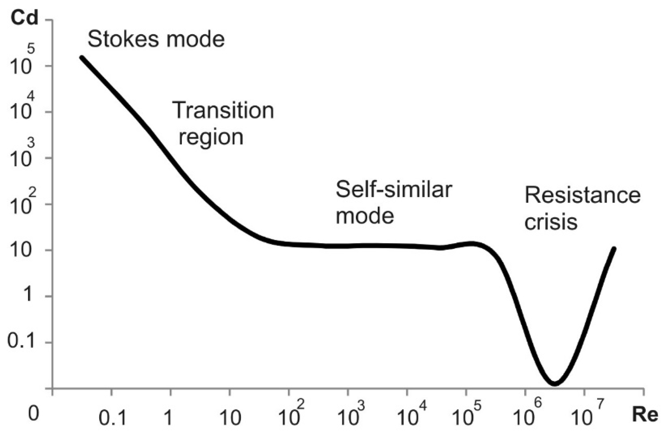
2.2.3. Drag Coefficient

The equation for describing the particle motion within the resisting medium includes the Reynolds number. It was early as Rayleigh who performed treatment of numerous experimental data to estimate the drag coefficient C_D of the solid sphere by Newton’s Equation (2). The treatment results are presented as the so-called standard drag curve in Figure 2. In some range of Re, the dependence of C_D(Re) is estimated analytically (Re < 1); in the other cases, C_D is calculated via an empirical formula derived by approximation of the measured data.

With low Reynolds numbers at Re < 1 corresponding to the laminar-flow regime, the drag coefficient of the solid spherical particle is expressed by the formula C_D = 24/Re, while the particle drag force in this regime is estimated by Equation (1). In a range of Re = 1−700, the transient-flow regime occurs. To describe the dependence of C_D(Re) in this regime, a whole set of empirical relationships are used that approximate the Rayleigh curves. Different studies obtained the dependences [30]:

$$\begin{array}{l}{C}_D=\frac{13}{\sqrt{\mathrm{Re}}},\\ C_D=\frac{24}{\mathrm{Re}}+\frac{4}{\sqrt[3]{\mathrm{Re}}},\\ C_D={\left(0.325+\sqrt{0.124+\frac{24}{\mathrm{Re}}}\right)}^2\end{array}$$

(3)

Those are the Allen formula, Klyachko formula, and Aerov–Todes formula, respectively [30,31].

In the turbulent-flow regime at Re = 700−3·10⁵, the drag coefficient remains constant: C_D = const. Specifically, C_D = 0.44 for the spherical particle. Such a flow regime is called self-similar. It is seen in Figure 2 that at some Re value (Re > 3·10⁵), the drag sharply diminishes. This phenomenon is called the Eiffel paradox [32,33] and stems from the fact that the boundary layer on the particle surface is turbulized. This effect is called the drag crisis [34].

2.2.4. Uniform Rectilinear Motion of a Particle—The Boussinesq Equation

Low Reynolds numbers. The differential equation that describes a one-dimensional motion of the particle within the viscous medium at Re < 1 was first derived by French mathematician and mechanic Boussinesq in 1903 [35]:

$$m_p\frac{d{u}_p}{dt}=F(t)-\frac{2}{3}\mathsf{\pi }{R}^3\mathsf{\rho }\frac{d{u}_p}{dt}-6\mathsf{\pi }\mathsf{\mu }R{q}_p-6R^2\sqrt{\mathsf{\pi }\mathsf{\mu }\mathsf{\rho }}{\displaystyle \underset{0}{\overset{t}{\int }}\frac{d{u}_p}{dx}}\frac{dx}{\sqrt{t-x}}.$$

(4)

where t is the time, x is the coordinate, m_p is the particle mass, and u_p is the particle motion velocity. Each of the terms on the right-hand side of Equation (4) has a certain physical sense.

The first term defines the external (gravitational, electrical, and so on) force F acting on the particle, and this force generally depends on time.

The second term is the energy inputs for bringing the medium into motion. It characterizes the resistance of the medium to the non-uniform motion of the spherical particle and represents an increase in the body mass by ½ that of the liquid (or gas) displaced by the particle. Since the gas density (ρ/ρ_p << 1) is much smaller than the particle density, this term is small for aerosols.

The third term describes the viscous medium resistance in case the particle moves at a constant speed equal to the velocity, as per the Stokes equation at the given instant of time.

The fourth term is again energy inputs for bringing the medium into motion. However, in contrast to the second term, this term (the integral) takes into account the inertia of the moving particles. It gives some decrease in the particle acceleration, with its value being not dependent on the viscosity of the medium but being dependent on the relation between the medium and particle densities: $\sqrt{\mathsf{\rho }/{\mathsf{\rho }}_p}$. Because the relation between the gas density and the condensed particle density is low, this term can be neglected with respect to aerosols.

Such an analysis of the Boussinesq equation peculiarities was undertaken by Fuchs [35]. This allowed him to make the important generalization: irrespective of the particle size, the particle motion can be considered principally inertialess. That is, the movement of a particle corresponds to the resistance of the medium at a constant motion velocity equal to the velocity value at the given moment of time.

Some of the terms in Equation (4) can be neglected at times that exceed the characteristic time of mechanical relaxation of the particle. In the case of low-Reynolds-numbers, the relaxation time is written as:

$$\mathsf{\tau }=\frac{m_p}{6\mathsf{\pi }\mathsf{\mu }R}=\frac{2}{9}\frac{R^2{\mathsf{\rho }}_p}{\mathsf{\mu }}.$$

(5)

If the particle motion is considered in the time intervals greater than time τ, it can be believed that from the very beginning, the particle moves at the stationary speed u_S. In other words, if we consider the particle motion with a greater duration (when compared to the mechanical relaxation time τ), the particle can be regarded as stationary relative to the medium (if no external forces act on it) or can be regarded as moving at a constant velocity u(t) = BF(t), where F(t) is the instantaneous value of external resultant forces and B is the particle mobility. Such a motion of the particles is called quasistationary (Fuchs [35]).

Mean and high Reynolds numbers. For the Reynolds number at Re > 1, the Boussinesq Equation (4) is not applicable, and the particle velocity cannot be considered stationary. Furthermore, the form of the analytical solution to the differential equation for particle motion is unknown. However, an analytical method for particle motion, in that case, was examined by Reist [11].

In the absence of external forces, the one-dimensional differential equation for particle motion is written as:

$$m_p\frac{d{u}_p}{dt}=F(t)+F_S(t).$$

(6)

The drag force can be expressed through the drag coefficient:

$$F_S(t)=C_D(\mathrm{Re})\cdot \mathsf{\pi }{R}^2\frac{\mathsf{\rho }{u}_p^2}{2}$$

Let us express the particle motion velocity u_p(t) via Re (by the definition of this criterion) and insert it together with the expression for force F_d(t) into Equation (6). The result is the following differential equation:

$$\frac{d\mathrm{Re}}{dt}=\frac{3}{16}\frac{\mathsf{\mu }}{{\mathsf{\rho }}_p{R}^2}{C}_D(\mathrm{Re}){\mathrm{Re}}^2.$$

(7)

After the integration of (7), the following system of equations is derived:

$$\begin{array}{l}t=\frac{16}{3}\frac{{\mathsf{\rho }}_p{R}^2}{\mathsf{\mu }}{\displaystyle \underset{{\mathrm{Re}}_1}{\overset{{\mathrm{Re}}_2}{\int }}\frac{d\mathrm{Re}}{C_D(\mathrm{Re}){\mathrm{Re}}^2}},\\ x=u_p(\mathrm{Re})t=\frac{8}{3}\frac{{\mathsf{\rho }}_p}{\mathsf{\rho }}R{\displaystyle \underset{{\mathrm{Re}}_1}{\overset{{\mathrm{Re}}_2}{\int }}\frac{d\mathrm{Re}}{C_D(\mathrm{Re})\mathrm{Re}}}.\end{array}$$

(8)

This system of equations determines the time and particle coordinate via the Re number and drag coefficient C_D(Re). As shown in Section 2.2.3, there is plenty of interpolation, empirical and theoretical formula to express the drag coefficient, which is based on multiple reliable experimental data (at least, obtained for spherical particles or particles with another simple shape). Having knowledge of these formulas, the time and particle coordinate can be numerically estimated as per Equation (8).

3. Aerosol Particle Motion in External Fields

3.1. Particle Motion under Gravity (the Stokes Mode)

In various practical problems, it is essential to know the motion regularities of dispersed particles (droplets, bubbles, solid particles) in the gravitational field. The gravitational sedimentation processes are important in estimating the particle propagation of harmful components originating from rocket accidents, to describe atmospheric precipitations, fogs, and clouds.

Let us look into the gravitational sedimentation of a spherical dispersed particle [36]. Direct the Oz axis downwards vertically; along the axial direction, the particle is affected by gravity force F_g = mg, Archimedes force F_A = –ρV_pg = –m_pρ/ρ_pg, where V_p is the volume of particle, and drag force of the environment $F_S(t)=C_D\mathsf{\pi }{R}^2\frac{\mathsf{\rho }{u}_p^2}{2}$.

In the Stokes mode, for which the conditions of Re < 1, C_D = 24/Re are met, the equation for sphere-shaped particle motion factoring in the forces takes the form:

$$\frac{d{u}_p}{dt}=g\left(1-\frac{\mathsf{\rho }}{{\mathsf{\rho }}_p}\right)-\frac{18\mathsf{\mu }}{{\mathsf{\rho }}_p{D}^2}{u}_p.$$

(9)

If the mode is stationary, $\frac{d{u}_p}{dt}=0$, the particle sedimentation rate is described by the formula:

$$u_s=\frac{\left({\mathsf{\rho }}_p-\mathsf{\rho }\right)D^2}{18\mathsf{\mu }}g.$$

(10)

Let us reduce Equation (9) to a dimensionless form. For that, the following scales have to be adopted: u_s (10) for velocity and $\mathsf{\tau }=\frac{D^2{\mathsf{\rho }}_p}{18\mathsf{\mu }}$ for time. Having specified the dimensionless variables y = u_p/u_s and θ = t/τ, we derive the following equation:

$$\frac{dy}{d\mathsf{\theta }}=1-y.$$

(11)

The initial condition for Equation (11) is θ = 0, y = 0, then the solution to the equation is written as:

$$y=1-e^{-\mathsf{\theta }}.$$

(12)

In its dimensionless form, the relationship between the particle velocity and time is depicted in Figure 3a.

The dynamic relaxation time of the particle is equivalent to θ = 1; within this time, the particle velocity will reach 0.63 of the stationary value of u_s. This value is indicated in the same Figure by the dotted line. The deviation of the sedimentation rate from the stationary one by 1% is attained at θ = 4.6.

To derive the particle velocity dependence of the drop height, we introduce the distance scale x_s = u_sτ; then the dimensionless coordinate will be written as ξ = x/x_s, while Equation (9) will have the form:

$$y\frac{dy}{d\mathsf{\xi }}=1-y.$$

(13)

The solution to Equation (13) with boundary conditions (ξ = 0: y = 0) has the form:

$$\mathsf{\xi }=-\left[y+\ln (1-y)\right].$$

(14)

The particle sedimentation rate plotted against the distance (drop height) in the dimensionless form is depicted in Figure 3b.

The particle velocity will reach 0.84 of the stationary value of u_s at the distance ξ = 1. The deviation of the velocity from the stationary one does not exceed 1% at ξ = 3.62.

3.1.1. Particle Motion Modes in the Gravitational Field

The regularities of the gravitational sedimentation of a particle assembly are generally studied by analytical or numerical modeling [35,37,38,39,40,41]. The verification of the theoretical models used requires experimental data on basic characteristics of the motion of a consolidated particle system. The literature on the experimental study into the sedimentation process of a particle cloud is limited [42,43,44,45].

The two particle motion modes under gravity can conditionally be discriminated:

1. Motion mode with acceleration. In this mode, the particle velocity grows gradually from zero to a constant value of u_s. Since u_p = u_s is attained only when time tends to infinity (τ→∞), we take the values θ = 4.6, ξ = 3.62 as the boundary of this mode when the deviation of the sedimentation rate from the stationary one does not exceed 1%. The corresponding dimensional values of the boundaries of this mode are defined by the formulas:

$$t_s=4.6\mathsf{\tau }=4.6\frac{{\mathsf{\rho }}_p{D}^2}{18\mathsf{\mu }};x_s=3.62x_s=3.62({\mathsf{\rho }}_p-\mathsf{\rho }){\left(\frac{D^2}{18\mathsf{\mu }}\right)}^{2}g.$$

(15)

In the accelerated motion mode, the particle sedimentation rate expressed as dimensional variables (D, μ, ρ, ρ_p, t) is defined by the formula:

$$u_p=\frac{({\mathsf{\rho }}_p-\mathsf{\rho })D^{2}g}{18\mathsf{\mu }}\left[1-\exp \left(-\frac{18\mathsf{\mu }}{{\mathsf{\rho }}_p{D}^2}t\right)\right].$$

(16)

2. Motion mode with constant velocityu_s. the particles travel at a stationary velocity as determined by the relation (10).

3.1.2. Calculation of Stationary Sedimentation of Particle via Criterion Equation

Let us consider the stationary sedimentation of a single spherical particle in the gravitational field: u_p = const. This is possible if the gravitational force and the Archimedes force are equilibrated by the drag force of the dispersed medium:

$$\frac{({\mathsf{\rho }}_p-\mathsf{\rho })\mathsf{\pi }{D}^{3}g}{6}=C_D\frac{\mathsf{\pi }{D}^2}{4}\frac{\mathsf{\rho }{u}_s^2}{2}.$$

(17)

The Reynolds number for the stationary sedimentation rate is $\mathrm{Re}=\frac{\mathsf{\rho }{u}_s^{}D}{\mathsf{\mu }}$, and the Archimedes number is $\mathrm{Ar}=\frac{g({\mathsf{\rho }}_p-\mathsf{\rho })\mathsf{\rho }{D}^3}{{\mathsf{\mu }}^2}$. Equation (17) using the data for dimensionless criteria can be presented in the form:

$${\mathrm{Re}}^2=C_D\frac{4}{3}\mathrm{Ar}.$$

(18)

As it follows from Equation (18), for the given particle motion mode, the Archimedes number and the Reynolds number are bound by the unique dependence (criterion Equation (18)). This equation is employed to estimate the particle’s steady-state velocity. The Archimedes number has to be calculated by the specified parameters of the problem (ρ, ρ_p, D, μ), and then the Reynolds number and the stationary particle sedimentation rate have to be estimated from Equation (18): $u_s=\mathrm{Re}\frac{\mathsf{\mu }}{\mathsf{\rho }D}$.

3.2. Aerosol Particle Coagulation

The gravitational field is a constant source of the aerosol particle motion on Earth. However, in practice, special exposures to external fields are used to remove (precipitate) aerosol particles. For instance, an intensive sound field (sirens) is exploited by sailors to eliminate fog; the electric field acts on dust particulates when an electric precipitator is turned on. Ultrafine aerosol particles are settled down by gravity very slowly, and special techniques for particle enlargement are often employed if they need to be removed from the air [46,47]. The particles can be eliminated from the air (gaseous medium) in two ways:

(1) By using their ability to coagulate (aggregate) with other particles and increase to such sizes at which they can settle rapidly in the gravitational field;

(2) By making the particles drift to the surfaces of sedimentation and settle them down over there.

Coagulation is an important process of aerosol particle interaction. It is viewed as the effects of aggregation, coalescence of particles when they move, and binary collisions. Triple and more-fold collisions are usually not considered, as these are unlikely. The coupling of liquid droplets is called “coalescence”, while the term “agglomeration” refers to solid particles.

Coagulation can be viewed as particle aggregation. These terms derive from aggrego (in Latin)–to herd together, and coagulatio (in Latin)–to curdle. The coagulation decreases the particle dispersity (enlargement), with a decrease in their number concentration at the same time.

The processes whereby the aerosol particles travel to each other or to the surface without any external exposures are called “diffusion” ones, while the motion of such particles in these processes is called the “Brownian motion”. Random collisions of the particles in such a motion result in their coagulation (natural Brownian coagulation). In other events, coagulation occurs under the action of external fields. The coagulation accelerated by external forces, when compared to the Brownian coagulation, is widely exploited in practice to entrap fine harmful aerosol particles, or in technological processes that use aerosols. In this case, different mechanisms of external exposure are more or less efficient (we consider the particle sedimentation time as the efficiency criterion) under different conditions. Coagulation is accelerated in turbulent flows [48], under the action of acoustic waves [49,50], under the combined action of ultrasound and vortex motion. Such a combined effect is successfully studied in the works of Khmelev et al. [51,52,53].

Estimating the duration of this sedimentation process is essential for determining the optimal conditions for the most efficient precipitation mechanism.

Based on previously published works with the participation of the authors, we consider various external fields and mechanisms by which they act on the aerosol particle precipitation.

3.2.1. External Electric Field and Acoustic Wind

Let us consider the characteristic times and precipitation rates of aerosol particles when exposed to the external field and without exposure.

When there are no external fields used, the particle settles down in the gravitational field. The stationary sedimentation rate is defined by Stokes Equation (10).

When exposed to the external electric field, the particle drifts towards the field source. The drift velocity of particles 1−50 µm wide is estimated by [54]:

$$u_{\mathrm{e}}=\frac{0.118\cdot {10}^{-10}D{E}^2}{2\mathsf{\mu }},$$

(19)

where E is the electric-field intensity [54]:

$$E=\sqrt{\frac{8iH}{4\mathsf{\pi }{\mathsf{\epsilon }}_0\mathsf{\epsilon }kd}},$$

i is the linear corona current density, d is the distance between the corona electrodes, H is the distance between the planes of the corona and precipitation electrodes, ε₀ is the electric constant, ε is the dielectric permittivity of the matter of particles, and k = 1.14·10⁻⁴ m²/(V·s) is the ion mobility.

When the acoustic exposure is powerful, the acoustic wind force acts on the particles. Let us consider the forces acting on the particle having diameter D in the acoustic field. These are the gravitational force, the air drag, and the radiation pressure force. If the radiation source is located above the particle, the radiation pressure force (P is the acoustic radiation pressure) is co-directional to the gravitational force. The radiation pressure force is $F_r=\mathsf{\pi }\frac{D^2}{4}P$.

By solving the equation for particle motion under the influence of the said forces, we derive a formula for the particle motion velocity, which includes contributions from the Stokes sedimentation velocity u_s and acoustic flow velocity u_w:

$$u_p=u_s+u_w=\frac{D^{2}g}{18\mathsf{\mu }}{\mathsf{\rho }}_p+\frac{PD}{12\mathsf{\mu }}.$$

(20)

The constituent of the particle motion velocity under acoustic wind is defined by:

$$u_w=\frac{PD}{12\mathsf{\mu }}.$$

(21)

In the traveling wave, the acoustic radiation pressure is defined by the sound pressure p:

$$P=\frac{2p^2}{\mathsf{\rho }{c}^2},$$

where c is the sound speed.

As seen from Equation (19), the motion velocity in the electric field is linearly dependent on the particle diameter, as is the velocity of particles entrained by the acoustic wind (21). The gravitational sedimentation rate (10) is proportional to the squared particle diameter.

So, we have three typical motion velocities of the particles in the environment: gravitational sedimentation velocity u_s (10), drift velocities under electrostatic field u_e (19), and under acoustic field u_w (21). The ratios of the velocities are different for different particle sizes. The drift velocity under the influence of electrostatic forces is 7.5 times as great as that under the acoustic wind for any particle size.

The drift velocity in the electric field is much greater than the gravitational sedimentation rate for smaller particles (1−5 µm), afterward, the difference diminishes, and the gravitational sedimentation becomes faster than the electric-field precipitation at some particle size. Such a particle size is defined by the relation: $D>\frac{1.062\cdot {10}^{-10}{E}^2}{\mathsf{\rho }g}$ or $\frac{D\mathsf{\rho }g}{E^2}>1.062\cdot {10}^{-10}$ and this expression determines the condition on which the use of an electroprecipitator makes sense.

The precipitation by the acoustic wind also occurs faster for smaller particles (1−3 µm), but when the particles’ diameter reaches ~ 6 µm, the gravitational sedimentation rate and the acoustic wind-induced precipitation rate become equal. Thus, the condition on which aerosol particles can be precipitated by the acoustic wind is derived from the condition u_w > u_s and looks like: $D>\frac{3P}{2g\left({\mathsf{\rho }}_p-\mathsf{\rho }\right)}$ or $\frac{2g\left({\mathsf{\rho }}_p-\mathsf{\rho }\right)D}{3P}>1$.

Thus, we have identified the two dimensionless groups: group $\frac{2g\left({\mathsf{\rho }}_p-\mathsf{\rho }\right)D}{3P}$ serves as the similarity criterion for the particle precipitation by the acoustic wind, while $\frac{D\mathsf{\rho }g}{E^2}$ is the similarity criterion for the electrostatic precipitation.

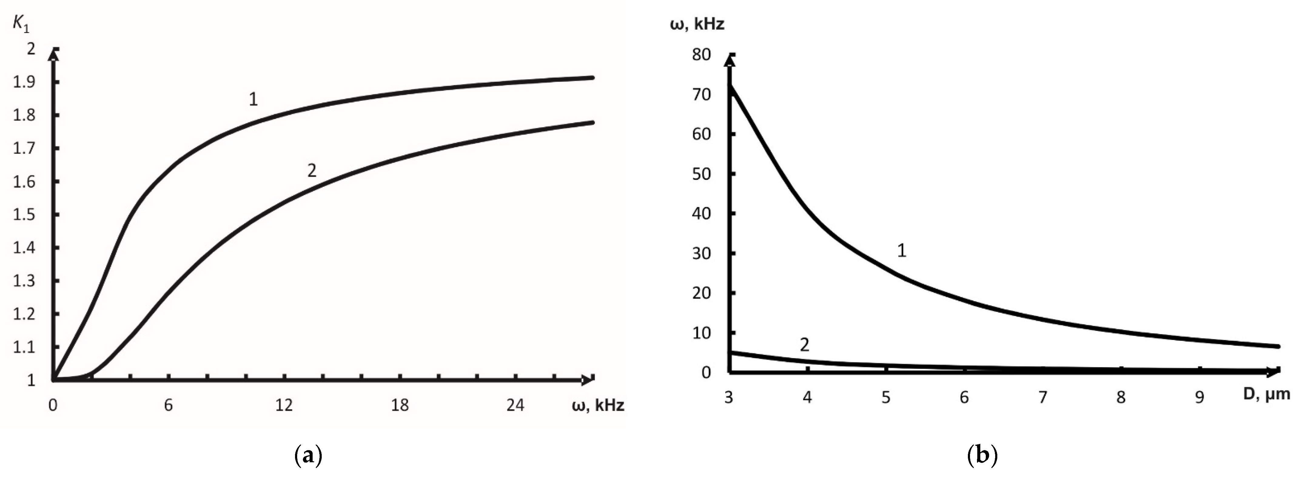
3.2.2. Acoustic Coagulation of Aerosol

The external forces cause the particles to move in a certain direction and settle down faster than when exposed to the gravitational forces. However, there is another way to accelerate the sedimentation―the coagulation (enlargement) of particles. The particles enlarged by coagulation settle down faster under gravity. Some types of external exposures can speed up this process. For instance, ultrasound exposure (acoustic) increases the particle coagulation rate [46,55]. Furthermore, an increase in the particle concentration (for example, by additional incorporation of a dispersed phase or by external aerosol field) and the presence of electrostatic charge on the particle surface promote the coagulation acceleration [56]. The coagulation rate is difficult to assess by analytical formulas according to the particle diameter. Integrodifferential equations and numerical modeling are employed to describe the coagulation process. The coagulation of particles of a polysize aerosol is described by the Smolukhovsky equation.

Let us look into the variation in the form of the particle size distribution in an aerosol cloud over time t. The variation in the mass distribution function of particle sizes is described by the balanced Smolukhovsky equation (in its integral form):

$$\frac{\partial g(D,t)}{\partial t}=I_1+I_2,$$

(22)

where the term I₁ is responsible for a decrement in a quantity of the particles having diameter D per unit time in unit volume due to the collision between the particle having diameter D and the particle having diameter D₁:

$$I_1=-g(D,t){\displaystyle \underset{0}{\overset{D_{\max }}{\int }}K(D,D_1)g(D_1,t)d}t,$$

(23)

where K(D, D₁) is the particle collision probability and D_max is the maximum diameter of the particles in the aerosol. The particles weighing more than the maximum value D_max(t) settle down by that time and are not further involved in coagulation. The D_max value can be evaluated by solving the problem of particle gravitational sedimentation: $D_{\max }=\sqrt{\frac{18\mathsf{\mu }H}{g\mathsf{\rho }t}},$ H is the upper boundary of the cloud (the height from which the particle of the said diameter falls down to the ground). The particle size distribution function is truncated on the right side due to the sedimentation of large particles. That boundary displaces gradually towards smaller and smaller particles over time.

The term I₂ is responsible for the emergence of particles having diameter D due to the collision of particles having diameters D₁ and D–D₁:

$$I_2=-\frac{1}{2}{\displaystyle \underset{0}{\overset{D}{\int }}K(D-D_1,D_1)f(D_1,t)f(D-D_1,t)d}t,$$

(24)

The initial conditions for Equation (22) are as follows: at t = t₀, f(D,t₀) = f₀(D) is the initial particle size distribution.

The core of integral Equations (23) and (24) is the particle collision probability K(D, D₁). The particle collision probability is determinant of the coagulation efficiency: the higher the particle collision probability, the faster the coagulation and aerosol settling. In the absence of external exposures, the coagulation is due to the Brownian motion. In the mathematical model (22) with no external exposures, the aerosol particle collision probability is assumed proportional to the summed projected frontal areas:

$$K(D,D_1)=\frac{k_b{n}_0}{\mathsf{\mu }}\left(D^2+D_1^2\right),$$

(25)

where k_b is the constant of proportionality, n₀ is the particle concentration.

Under ultrasonic exposure, the particle collision probability rises. The parameters that describe the ultrasonic exposure–these are, first of all, radiation frequency and amplitude–should be included in Equation (25).

The coagulation in the acoustic field occurs as a result of the particles’ interaction evoked by acoustic streams around the particles [57]. The number of collisions is proportional to the squared particle motion velocity, cross-sectional area, particle concentration, and flow coefficient k_flow, and is inversely proportional to the environment viscosity:

$$N\approx \frac{u_p^2{n}_0^{}{k}_{flow}^2(D^2+D_1^2)}{\mathsf{\mu }}.$$

(26)

In that case, the particle motion velocity is defined by the amplitude of acoustic vibrations. In line with the orthokinetic hypothesis, the particle when exposed to the acoustic forces is dragged into the vibratory motion. Subject to the environment properties and particle’s density and sizes, the environment can entrain the particle better or worse. This is determined by the entrainment coefficient k_entr–the relation between the particle velocity amplitude and the dispersed medium velocity amplitude. The Reynolds number for the processes of interest is small, therefore it can be thought that the Stokes force is effective between the medium and the particle. Then the formula for the entrainment coefficient is:

$$k_{entr}=\frac{1}{\sqrt{1+{\mathsf{\omega }}^2{\mathsf{\tau }}^2}},$$

(27)

where ω is the sound vibration frequency and $\mathsf{\tau }={\mathsf{\rho }}_p{D}^2/18\mathsf{\mu }$ is the time of the mechanical relaxation of the particle. It follows from the analysis of Equation (27) that the higher the particle’s density and size, and the higher the vibrational frequency and the lower the viscosity of the medium, the greater the difference of the particle vibration amplitude from the gas vibration amplitude.

Equation (27) shows that the particle entrainment by the acoustic field results in a higher collision probability between that particle and the other one by $k_{flow}^2=k_a{(1-k_{entr})}^2$ times, where k_a is the constant of proportionality. From hence, one can derive an equation for collision probability of the particles having diameters D and D₁, given that it is proportional to N·(1–k_entr)², taking into account Equations (25)–(27):

$$K(D,D_1)=\frac{k_b{n}_0^{}}{\nu }(D^2+D_1^2)\left(1+k_a{u}_p^2{\left(1-\frac{1}{\sqrt{1+{\mathsf{\omega }}^2{\mathsf{\tau }}^2}}\right)}^2\right).$$

(28)

The analysis of Equation (28) allows the following to be found out:

• If there is no acoustic field, i.e., $k_a{u}_p^2$ = 0, then the collision probability is defined by the Brownian motion (25);
• if the vibrational amplitude rises and hence the velocity up, the collision probability increases;
• the sound field with relatively low frequencies (ω²τ² << 1) almost does not increase the collision probability as well, (k_entr →1, (1– k_entr) →0);
• if the sound vibration frequency is ω²τ² >> 1, the probable collisions and aerosol coagulation take place to maximum effect: k_entr →0, (1– k_entr) →1.

Based on the asymptotic analysis of Equation (28), we will find the minimal (at ω²τ² << 1) and maximal (at ω²τ² >> 1) frequencies of the acoustic exposure:

$${\mathsf{\omega }}_{\min }=\frac{1}{\mathsf{\tau }}\left[1/{\left(1-\frac{\mathit{o}\left(\sqrt{k_b{n}_0{D}_0^2}\right)}{u_p\sqrt{k_a}}\right)}^2-1\right],$$

(29)

$${\mathsf{\omega }}_{\max }=\frac{1}{\mathsf{\tau }}\left[\frac{1}{\mathit{o}(1)}-1\right].$$

(30)

Here, o(f(x)) denotes “the infinitesimal relative to f(x)”, and f(x) is some function. This denotation was taken to compare the asymptotic behavior of the functions. In practice, one can take the 1% value as the “infinitesimal” approximation (as was performed in Section 3.1 when considering the particle motion in the gravitational field). Then, o(f(x)) = 0.99 f(x) and o(1) = 0.99. Then, Equations (29) and (30) take the form:

$${\mathsf{\omega }}_{\min }=\frac{1}{\mathsf{\tau }}\left[1/{\left(1-\frac{0.99\left(\sqrt{k_b{n}_0{D}_0^2}\right)}{u_p\sqrt{k_a}}\right)}^2-1\right]$$

(31)

$${\mathsf{\omega }}_{\max }=\frac{1}{\mathsf{\tau }}\left[\frac{1}{0.99}-1\right]\approx \frac{0.01}{\mathsf{\tau }}.$$

(32)

Note that if the value of 0.1% is taken as an “infinitesimal” approximation, then ${\mathsf{\omega }}_{\max }\approx 0.001/\mathsf{\tau },$ and so on. Therefore, this approximation is conditional.

It can be noted by comparing Equations (27) and (30) that there is a dimensionless group responsible for multiplying the collision probability of the particles when exposed to the acoustic field: $K_1=\left(1+k_a{u}_p^2{\left(1-\frac{1}{\sqrt{1+{\mathsf{\omega }}^2{\mathsf{\tau }}^2}}\right)}^2\right)$. Depending on the frequency, the multiplying factor behaves itself the way as shown in Figure 4a (calculation for aqueous aerosol, $k_a{u}_p^2$ = 1, μ = 18.1·10⁻⁶ Pa·s–dynamic viscosity of air, ρ_p = 1000 kg/m³–the density of water). The calculation results for minimal and optimal frequencies of the exposure for the aqueous aerosol by Equations (31) and (32) are displayed in Figure 4b.

3.2.3. Aerosol Coagulation with an Additional Dispersed Phase Incorporated

It follows from Equation (28) that the smaller the particles’ diameter and hence the relaxation time τ, the higher frequency ω is required to elevate the coagulation rate. However, the acoustic and Brownian coagulations can be accelerated if the particle concentration n₀ is raised, as it follows from Equations (25) and (28). The particle concentration can be raised if one incorporates additional coagulation sites into the existing aerosol, i.e., atomizes an additional portion of the aerosol. The higher the dispersity of the aerosol incorporated, the more the coagulation centers at the same particle weight. The greater the particle concentration n₀, the higher the number of collisions per unit time and the higher the coagulation rate and hence the sedimentation rate.

The coagulation model (22) described hereinabove has to be accompanied by the initial condition of the following form in order to take into account the second phase [58]:

$$f_0(D)=a[(1-\mathsf{\delta })D^{\alpha }\exp (-bD)+\mathsf{\delta }{D}^{{\alpha }_1}\exp (-b_{1}D)],$$

where the distribution parameters with index 1 relate to the additional dispersed phase; and δ is the proportion of the particles of the additional aerosol. The expression for collision probability when the additional aerosol is incorporated takes the following form:

$$K(D,D_1)=\frac{k_b{n}_0^{}}{{\mathsf{\mu }}^{}}\left(\frac{1}{1-\mathsf{\delta }}\right)\left(D^2+D_1^2\right).$$

(33)

The additional dispersed phase can be represented by electrostatically charged solid particles. Then, the particle charge value should be included in the expression for particle collision probability.

Let the powder particles have the charge q and diameter D, while the particles of the initial aerosol having diameter D₁ will acquire the opposite charge q₁ as a result of the electrostatic induction phenomenon. The Coulomb force acts on the opposite-charged particles: $F_C=k_C\frac{q_1{q}_2}{r_{12}^2},$ where r₁₂ is the distance between the particles, $k_C=1/(4\mathsf{\pi }{\mathsf{\epsilon }}_g{\mathsf{\epsilon }}_0)$ and ε_g is the relative dielectric permittivity of the medium.

The steady-state particle velocity u_e factoring in the friction and Coulomb forces is $u_e=\frac{k_C}{3\mathsf{\mu }}\frac{q_{1}q}{r_{12}^2{D}_1},$ while the particle collision probability will be:

$$K(D,D_1)=\frac{k_b{n}_0^{5/3}{\left(q_{1}q\right)}^2}{9{\mathsf{\mu }}^3}\left(\frac{1}{1-\mathsf{\delta }}\right)\left(1+{\left(\frac{D}{D_1}\right)}^2\right).$$

(34)

One can note the following by comparing the expressions for the core of the Smolukhovsky equation in the form of (28) (for acoustic exposure) and in the form of (34) (electrostatic coagulation):

• the collision probability dependence of the particle concentration under electrostatic coagulation is stronger than under the acoustic one;
• the collision probability (and coagulation rate) dependence of the gaseous medium viscosity is also stronger under electrostatic coagulation;
• the greater the electrostatic charge of the particle and the lower the dielectric permittivity, the higher the collision probability in the case of electrostatic coagulation.

3.3. Aerosol Precipitation Rates in External Fields

Table 1. Ratios of characteristic motion velocities of particles under different exposures.

D, µm	ue/us	uw/us	uus/us
1	46.1	6.14	55.1
2	23.0	3.07	27.5
3	15.4	2.05	18.2
4	11.5	1.54	13.6
5	9.21	1.23	10.6
6	7.68	1.02	8.28
7	6.58	0.877	6.43
8	5.76	0.767	5.06
9	5.12	0.682	4.09
10	4.61	0.614	3.38
11	4.19	0.558	2.85
12	3.84	0.512	2.44
13	3.54	0.472	2.12
14	3.29	0.439	1.86
15	3.07	0.409	1.65

summarizes the estimation results regarding the particle motion velocity for different precipitation mechanisms. The estimation was performed for coal particles (ρ_p = 1300 kg/m³). The gravitational sedimentation rate u_s was calculated by Equation (10), the particle velocity in the electrostatic field u_e by Equation (19), the particle velocity in the acoustic stream u_w by Equation (21), and the acoustic coagulation-induced precipitation rate u_us was derived from a numerical solution to Equation (22).

Figure 5 displays the precipitation of particles plotted against particle sizes for different precipitation mechanisms.

If the gravity-mediated velocity component u_s is higher than the radiation force-mediated velocity component u_w, then the leading mechanism is the Stokes sedimentation. Otherwise, if u_w > u_s, the leading precipitation mechanism is the acoustic wind which “blows off” the particles down to the test chamber bottom. If the particle sizes increase, the Stokes sedimentation becomes the leading mechanism because the particle weight is decisive.

The natural gravitational sedimentation and the acoustic stream-induced motion are the slowest precipitation mechanisms. It can be noticed by comparing them that the small particles such as air-suspended coal dust having a particle diameter below 6 µm are faster to be “blown off” by the acoustic wind than they are settled by gravity.

The higher the vibrational frequency, the faster the acoustic coagulation (Section 3.2.2). Under the acoustic exposure conditions, two mechanisms are effective at the same time: enlargement of particles and acoustic streaming. Starting from some fairly large particle size (in our case, a diameter of about 18 µm), the acoustic coagulation and precipitation are slower than the natural gravitational.

For smaller particles having a diameter below 6 µm, the acoustic coagulation rate is somewhat higher than in the electrostatic field. The larger particles move in the electrostatic field considerably faster than under the other external forces.

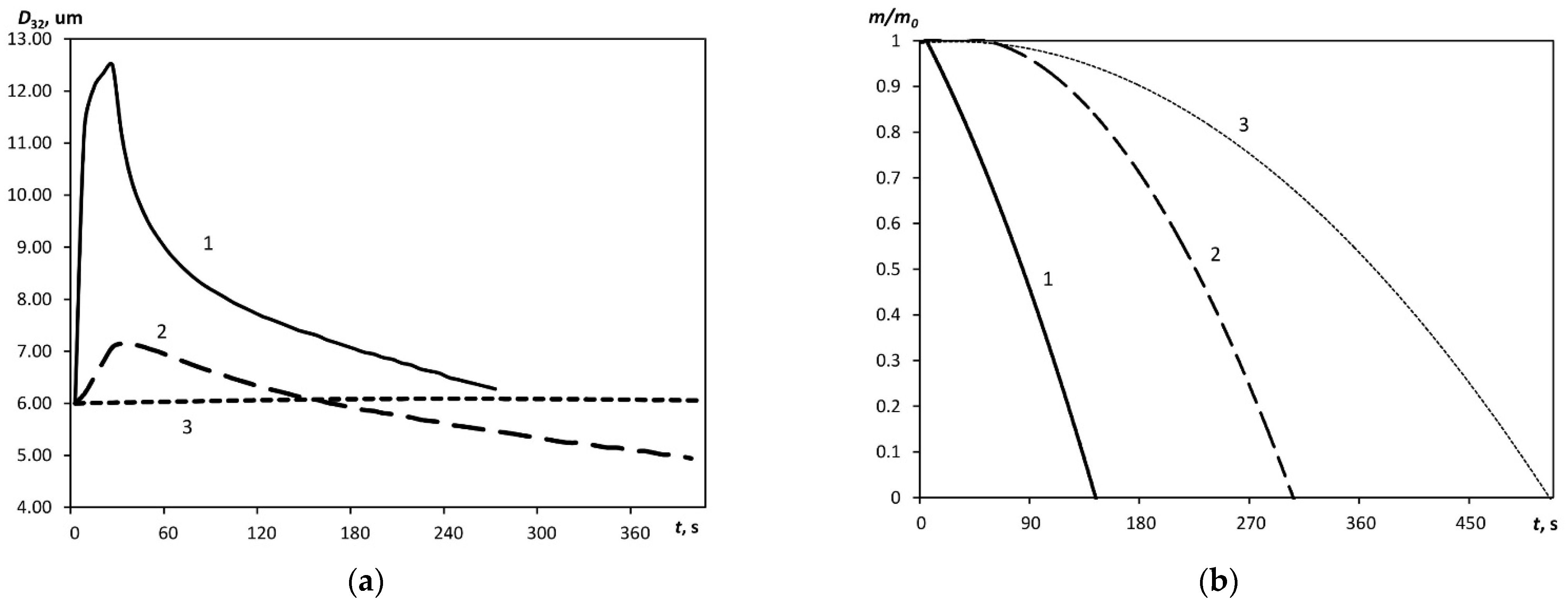
Variations in Particle Sizes and Aerosol Weight in External Fields

Figure 6a demonstrates the time course of the Sauter diameter of the particles under electrostatic coagulation, ultrasound coagulation, and Brownian coagulation (no exposure). In case the particles are electrostatically charged, they coagulate very fast within a dozen seconds, whereupon they begin to settle down, and the size of the particles still suspended in the air declines gradually. In the case of ultrasound coagulation, the enlargement of the particles is much slower, and the particles are enlarged not so much like in the case of electrostatic charging. Without exposure, the particles’ diameter almost does not alter all the time.

The estimations were carried out for the system of Equation (22). The core of integral Equations (23) and (24) was chosen in the form of (28) for the ultrasound coagulation and in the form of (34) for the electrostatic coagulation.

Figure 6b illustrates the time course of the relative particle concentration m/m₀ for all three cases of interest.

The small coal particles settle down without exposure for about 8 min. The ultrasound exposure speeds up this process significantly whereby the sedimentation occurs within 5 min. When a portion of powder with the electrostatically charged surface is atomized, the precipitation rate shortens to 2–3 min.

4. Conclusions

Here we have looked into the aerosol media behavior and the motion of aerosol particles and assemblies thereof, including the motion under the influence of external fields and in the presence of electrostatically charged particles. In addition, we have adduced the main classical similarity criteria used in the aerosol mechanics, as well as less common similarity criteria used to describe particular cases of particle motion in external fields. The presence of similarity criteria is the manifestation of physical symmetry in aerodispersed systems and enables the relationship between physical parameters to be established when describing the aerosol particle motion.

The precipitation of finely dispersed aerosols poses a problem. Different techniques are employed to tackle this problem. We have considered the estimation results for characteristic precipitation rates of fine aerosols when exposed to the ultrasonic field, electric field, acoustic streaming, and gravitational sedimentation. The ratios of the velocities, as well as dimensionless groups (Section 3.2.1), allow the leading precipitation mechanism to be identified. The precipitation of fine particles by the electrofilter is efficient for relatively larger particles (by an example of coal particles, above 6 µm). The acoustic precipitation was efficient for particles having a diameter below 18 µm, as compared to gravitational sedimentation; larger particles are also fast to settle down in the gravitational field. The acoustic wind is the least important precipitation mechanism among those considered. It helps settle down the finest particles (below 3 µm).

The precipitation of aerosol particles by ultrasound relies on the ultrasound coagulation phenomenon. However, there is a possibility to make the particles coagulate faster without external fields applied. For this, electrostatically charged particles should be atomized in the air, which will attract harmful agent particles. Electrostatic coagulation is more efficient for relatively high concentrations of particles having smaller sizes.

References

1. Meszaros, E. Fundamental of Atmospheric Aerosol Chemistry; Ak. Kiado: Budapest, Romania, 1999. [Google Scholar]
2. Pope, C.A., III; Bhatnagar, A.; McCracken, J.P.; Abplanalp, W.; Conklin, D.J.; O’Toole, T. Exposure to Fine Particulate Air Pollution Is Associated with Endothelial Injury and Systemic Inflammation. Circ. Res. 2016, 119, 1204–1214. [Google Scholar] [CrossRef] [PubMed] [Green Version]
3. Atkinson, R.; Kang, S.; Anderson, H.; Mills, I.; Walton, H. Epidemiological time series studies of PM2. 5 and daily mortality and hospital admissions: A systematic review and meta-analysis. Thorax 2014, 69, 660–665. [Google Scholar] [CrossRef] [PubMed] [Green Version]
4. Xing, Y.F.; Xu, Y.H.; Shi, M.H.; Lian, Y.X. The impact of PM2.5 on the human respiratory system. J. Thorac. Dis. 2016, 8, E69. [Google Scholar] [PubMed]
5. Pope, C.A., III; Burnett, R.T.; Thun, M.J.; Calle, E.E.; Krewski, D.; Ito, K.; Thurston, G.D. Lung cancer, cardiopulmonary mortality, and long-term exposure to fine particulate air pollution. JAMA 2002, 287, 1132–1141. [Google Scholar] [CrossRef] [Green Version]
6. Kumar, R.; Barth, M.C.; Pfister, G.G.; Delle Monache, L.; Lamarque, J.F.; Archer-Nicholls, S.; Walters, S. How will air quality change in South Asia by 2050? J. Geophys. Res. Atmos. 2018, 123, 1840–1864. [Google Scholar] [CrossRef]
7. Eber, M. Smoke separators to reduce air pollution. CZ Chem. Tech 1977, 6, 523–527. [Google Scholar]
8. Rohilla, M.; Saxena, A.; Dixit, P.K.; Mishra, G.K.; Narang, R. Aerosol forming compositions for fire fighting applications: A review. Fire Technol. 2019, 55, 2515–2545. [Google Scholar] [CrossRef]
9. Altshuller, A.P.; Bufallini, J.J. Photochemical aspects of air pollution. Environm. Sci. Technol. 1971, 5, 39–63. [Google Scholar] [CrossRef]
10. Reid, J.P.; Sayer, R.M. Chemistry in the clouds: The role of aerosols in atmospheric chemistry. Sci. Prog. 2002, 85, 263. [Google Scholar]
11. Reist, P.C. Introduction to Aerosol Science; Macmillan Publishing Company: New York, NY, USA, 1984. [Google Scholar]
12. Green, H.L.; Lane, W.R. Particulate Clouds: Dusts, Smokes and Mists. Their Physics and Physical Chemistry and Industrial and Environmental Aspects; E. & F.N. Spon, Ltd.: London, UK, 1957. [Google Scholar]
13. Sedov, L.I. Similarity and Dimensional Methods in Mechanics; CRC Press: Boca Raton, FL, USA, 1993. [Google Scholar]
14. Clift, R.; Grace, J.R.; Weber, M.E. Bubbles, Drops and Particles; Dover Publications: Mineola, NY, USA, 1978; p. 380. [Google Scholar]
15. Crowe, C.T.; Sommerfeld, M.; Tsuji, Y. Multiphase Flows with Droplets and Particles; CRC Press: Boca Raton, FL, USA, 1998; p. 471. [Google Scholar]
16. Michaelides, E.E. Bubbles, Drops and Particles: Their Motion, Heat and Mass Transfer; World Scientific: Singapore, 2006; p. 410. [Google Scholar]
17. Pai, S.I. Two-Phase Flows; Springer: Berlin/Heidelberg, Germany, 2013. [Google Scholar]
18. Hidy, G.M.; Brock, J.R. The Dynamics of Aerocolloidal Systems: International Reviews in Aerosol Physics and Chemistry; Elsevier: Amsterdam, The Netherlands, 2016; Volume 1. [Google Scholar]
19. Hidy, G.M. (Ed.) Topics in Current Aerosol Research: International Reviews in Aerosol Physics and Chemistry; Elsevier: Amsterdam, The Netherlands, 2016; Volume 3. [Google Scholar]
20. Williams, M.M.R.; Loyalka, S.K. Aerosol Science: Theory and Practice; Pergamon Press: Oxford, UK, 1991. [Google Scholar]
21. Brennen, C.E. Fundamentals of Multiphase Flows; Cambridge University Press: Cambridge, UK, 2005. [Google Scholar]
22. Hinds, W.C. Aerosol Technology: Properties, Behavior, and Measurement of Airborne Particles, 2nd ed.; Wiley-Interscience: Hoboken, NY, USA, 1999. [Google Scholar]
23. Seinfeld, J.H.; Pandis, S.N. Atmospheric Chemistry and Physics: From Air Pollution to Climate Change; Wiley-Interscience: Hoboken, NY, USA, 1998. [Google Scholar]
24. Kuznetsov, G.V.; Strizhak, P.A.; Shlegel, N.E. Interaction of water and suspension droplets during their collisions in a gas medium. Theor. Found. Chem. Eng. 2019, 53, 769–780. [Google Scholar] [CrossRef]
25. Pesin, Y.B. Dimension Theory in Dynamical Systems: Contemporary Views and Applications; University of Chicago Press: Chicago, IL, USA, 2008. [Google Scholar]
26. Sterrett, S.G. Similarity and dimensional analysis. In Philosophy of Technology and Engineering Sciences; Elsevier: Amsterdam, The Netherlands, 2009; pp. 799–823. [Google Scholar]
27. Gukhman, A.A. Introduction to Similarity Theory; Vysshaya Shkola Publisher: Moscow, Russia, 1973; p. 296. (In Russian) [Google Scholar]
28. Arkhipov, V.A.; Berezikov, A.P. Theory Bases of Engineering and Physical Experiments; Tomsk Polytechnic University Publisher: Tomsk, Russia, 2008; p. 206. (In Russian) [Google Scholar]
29. Beresnev, S.A.; Gryazin, V.I. Physics of Atmospheric Aerosols; Ural University Publisher: Yekaterinburg, Russia, 2008; p. 227. (In Russian) [Google Scholar]
30. Nigmatulin, R.I.; Friedly, J.C. Dynamics of Multiphase Media; CRC Press: Boca Raton, FL, USA, 1990; Volume 2. [Google Scholar]
31. Sternin, L.E.; Maslov, B.N.; Shraiber, A.A.; Podvysotskii, A.M. Two-Phase Mono-and Polydisperse Gas Flows Containing Particles; Izdatel Mashinostroenie: Moscow, Russia, 1980. [Google Scholar]
32. Eiffel, G. Sur la résistance des sphères dans l’air en movement. Comptes Rendus 1912, 155, 1597–1599. [Google Scholar]
33. Prandtl, L. Gesammelte Abhandlungen zur Angewandten Mechanik, Hydro-und Aerodynamik: T. Chronologische Folge der Veröffentlichungen. Elastizität, Plastizität, Rheologie. Tragflügel und Luftschrauben; Springer: Berlin/Heidelberg, Germany, 1961. [Google Scholar]
34. Stoker, J.J. Garrett Birkhoff, Hydrodynamics, a study in logic, fact, and similitude. Bull. Am. Math. Soc. 1951, 57, 497–499. [Google Scholar] [CrossRef]
35. Fuks, N.A. The Mechanics of Aerosols; Academy of Science Publisher: Moscow, Russia, 1955. [Google Scholar]
36. Levich, V.G.; Tobias, C.W. Physicochemical hydrodynamics. J. Electrochem. Soc. 1963, 110, 251. [Google Scholar] [CrossRef]
37. Ekiel-Jezewska, M.L.; Metzger, B.; Guazzelli, E. Spherical cloud of point particles falling in a viscous liquid. Phys. Fluids 2006, 18, 038104. [Google Scholar] [CrossRef] [Green Version]
38. Yin, X.; Koch, D.L. Hindered settling velocity and microstructure in suspensions of solid spheres with moderate Reynolds numbers. Phys. Fluids 2007, 19, 093302. [Google Scholar] [CrossRef]
39. Abade, G.C.; Cunha, F.R. Computer simulation of particles aggregates during sedimentation. Comput. Methods Appl. Mech. Eng. 2007, 196, 4597–4612. [Google Scholar] [CrossRef]
40. Subramanian, G.; Koch, D.L. Evolution of clusters of sedimenting low-Reynolds-number particles with Oseen interactions. J. Fluid Mech. 2008, 603, 63–100. [Google Scholar] [CrossRef]
41. Zaidi, A.A.; Tsuji, T.; Tanaka, T. A new relation of drag force for high Stokes number monodisperse spheres by direct numerical simulation. Adv. Powder Technol. 2014, 25, 1860–1871. [Google Scholar] [CrossRef]
42. Nitsche, L.C.; Batchelor, G.K. Break-up of a falling drop containing dispersed particles. J. Fluid Mech. 1997, 340, 161–175. [Google Scholar] [CrossRef]
43. Machu, G.; Meile, W.; Nitsche, L.C.; Schaflinger, U. Coalescence, torus formation and breakup of sedimenting drops: Experiments and computer simulation. J. Fluid Mech. 2001, 447, 299–336. [Google Scholar] [CrossRef] [Green Version]
44. Metzger, B.; Nicolas, M.; Guazzelli, E. Falling clouds of particles in viscous fluids. J. Fluid Mech. 2007, 580, 283–301. [Google Scholar] [CrossRef]
45. Mylyk, A.; Meile, W.; Brenn, G.; Ekiel-Jezewska, M.L. Break-up of suspension drops settling under gravity in a viscous fluid close to a vertical wall. Phys. Fluids 2011, 23, 063302. [Google Scholar] [CrossRef] [Green Version]
46. Khmelev, V.N.; Shalunov, A.V.; Shalunova, K.V. The acoustical coagulation of aerosols. In 2008 9th International Workshop and Tutorials on Electron Devices and Material; IEEE: Piscataway, NJ, USA, 2008; pp. 289–294. [Google Scholar]
47. Stepkina, M.Y.; Kudryashova, O.B.; Antonnikova, A.A.; Zhirnov, A.A. Application of Electrostatic Effect for Cleansing Finely Divided Aerosol from Air. J. Eng. Phys. Thermophys. 2020, 93, 796–801. [Google Scholar] [CrossRef]
48. Yang, H.; Lin, J.; Chan, T. Effect of Fluctuating Aerosol Concentrations on the Aerosol Distributions in a Turbulent Jet. Aerosol Air Qual. Res. 2020, 20, 1629–1639. [Google Scholar] [CrossRef] [Green Version]
49. Liu, C.; Zhao, Y.; Tian, Z.; Zhou, H. Numerical simulation of condensation of natural fog aerosol under acoustic wave action. Aerosol Air Qual. Res. 2021, 21, 200361. [Google Scholar] [CrossRef]
50. Lu, M.; Fang, M.; He, M.; Liu, S.; Luo, Z. Insights into agglomeration and separation of fly-ash particles in a sound wave field. RSC Adv. 2019, 9, 5224–5233. [Google Scholar] [CrossRef] [Green Version]
51. Khmelev, V.N.; Shalunov, A.V.; Nesterov, V.A. Improving the separation efficient of particles smaller than 2.5 micrometer by combining ultrasonic agglomeration and swirling flow techniques. PLoS ONE 2020, 15, e0239593. [Google Scholar] [CrossRef]
52. Khmelev, V.N.; Nesterov, V.A.; Bochenkov, A.S.; Shalunov, A.V. The Limits of Fine Particle Ultrasonic Coagulation. Symmetry 2021, 13, 1607. [Google Scholar] [CrossRef]
53. Khmelev, V.N.; Shalunov, A.V.; Golykh, R.N. Increasing the Efficiency of Coagulation of Submicron Particles under Ultrasonic Action. Theor. Found. Chem. Eng. 2020, 54, 539–550. [Google Scholar] [CrossRef]
54. Uzhov, V.N. Cleaning Industrial Gases with Filters; Chemistry: Moscow, Russia, 1967; p. 344. (In Russian) [Google Scholar]
55. Kudryashova, O.; Korovina, N.; Akhmadeev, I.; Muravlev, E.; Titov, S.; Pavlenko, A. Deposition of Toxic Dust with External Fields. Aerosol Air Qual. Res. 2018, 18, 2575–2582. [Google Scholar] [CrossRef] [Green Version]
56. Kudryashova, O.; Stepkina, M.; Antonnikova, A. New Ways to Use Charged Particles. In Advances in Chemistry Research; Nova Science Publishers, Inc.: Hauppauge, NY, USA, 2019; Volume 61. [Google Scholar]
57. Rosenberg, L.L. Physics and Engineering of Powerful Ultrasound. In Powerful Ultrasound Fields; Nauka Publisher: Moscow, Russia, 1968; Volume 2, p. 258. (In Russian) [Google Scholar]
58. Titov, S.; Stepkina, M.; Antonnikova, A.; Korovina, N.; Vorozhtsov, B.; Muravlev, E.; Kudryashova, O. Sedimentation of harmful dust by means of ultrasonic waves and additional disperse phase. Arab. J. Geosci. 2015, 8, 11321–11328. [Google Scholar] [CrossRef]
Figure 1. Regimes of the gas flow around the spherical particle.
Symmetry 14 00363 g001
Figure 2. The drag coefficient plotted against the Reynolds criterion.
Symmetry 14 00363 g002
Figure 3. Particle sedimentation rate in the gravitational field plotted against (a) time and (b) distance.
Symmetry 14 00363 g003
Figure 4. (a) Multiplying factor K1 (dimensionless group) plotted against acoustic exposure frequency for aqueous aerosol: (1) D = 5 µm; (2) D = 1 µm. (b) (1) Maximal ωmax and (2) minimal ωmin acoustic frequencies for coagulation of aqueous aerosol particles.
Symmetry 14 00363 g004
Figure 5. The precipitation rate according to different mechanisms (gravitational, acoustic stream, electric field, ultrasonic field) plotted versus the particle diameter.
Symmetry 14 00363 g005
Figure 6. The time course of (a) Sauter diameter and (b) relative concentration: 1. electrostatic coagulation, 2. ultrasound coagulation, 3. Brownian coagulation (no exposure).
Symmetry 14 00363 g006