Numerical Investigation of the Automatic Air Intake Drag Reduction Strut Based on the Venturi Effect

Abstract

Drag reduction by injecting air is a promising engineering method for improving ship performance. A novel automatic air intake drag reduction strut structure based on the Venturi effect is proposed for the high-speed small water-plane area twin hull vessels in the present study. The drag reduction strut can achieve the function of automatic air intake when the vehicle is moving at high speed, and the air inhaled and the incoming flow form bubbly flows to cover the strut surface, effectively reducing the drag of the strut. Considering the longitudinal symmetry of the strut structure, a two-dimensional single-chip drag reduction strut structure is designed to facilitate analysis and a solution. The volume of fluid model is combined with the k-ω SST turbulence model, and a numerical simulation is carried out to investigate the variation of the air inflow, the air volume fraction in the bubbly flows of the strut and the drag reduction rate of the strut for different sailing speeds. The analysis result shows that when the proposed model reaches a certain speed, the external air is inhaled by the strut intake duct, and the bubbly flows are formed with the incoming flow covering the surface of the strut, thereby reducing the drag coefficient. Meanwhile, it is found that as the sailing speed increases, the drag reduction rate of the strut gradually rises and its maximum value reaches about 30%. For high sailing speeds, the drag reduction rate is affected by wave-making resistance so that it gradually declines.

1. Introduction

A new type of high-speed surface vehicle similar to the small water-plane area twin hull (SWATH) [1] has attracted people’s attention. Forming supercavities on the SWATH vessels via artificial ventilation can lower resistance by reducing the wetting surface of the submerged bodies by applying supercavitation techniques [2]. However, as the strut passes through the water, supercavities cannot be formed on its surface. The skin friction drag of the strut surface can account for almost half of the total drag of the ship. Considering the effects of skin friction drag of the strut on the total resistance of the vehicle, drag reduction by bubbly flows is an effective way of strut drag reduction.

Various methods have been explored to reduce the skin friction drag in the past. One such method—drag reduction by bubbly flows—has recently become a focus in the expectation that it might be applicable to ships. Early reporting of drag reduction by bubbly flows was by Mccormick [3]. They observed viscous drag reduction of a fully submerged body by creating hydrogen gas on the hull by electrolysis. Murai [4] developed the study of the mechanism of drag reduction using relatively large air bubbles compared to the boundary layer thickness in a horizontal turbulent channel flow and indicated that there is a negative correlation between the local skin friction and the local void fraction.

A common method to form bubbly flows is gas injection into the liquid boundary layer. Such injection results in the formation of bubbles that produce drag reduction. Drag reduction by injecting air can be categorized into microbubble drag reduction (MBDR) and air layer drag reduction (ALDR), according to the shape and distribution of air bubbles.

In MBDR, a number of experiments and numerical studies have been carried out to investigate. Madavan et al. [5] indicated that microbubbles can cause a reduction of high-frequency shear-stress fluctuations and a destruction of some of the turbulence in the near-wall region by spectral measurements. Kodama et al. [6] carried out the microbubble experiments using a circulating water tunnel specially designed for microbubble experiments, and skin friction reduction by microbubbles of up to 40% was obtained. Sayyaadi et al. [7] estimated a simple formulation for calculating an efficient injection rate by considering the main parameters of the ship by the model test results of a 70 cm catamaran model. The test results showed that excessive air injection decreases the drag reduction effect, while suitable injection reduces total drag by about 5–8%. Paik et al. [8] developed the study of a bubbly turbulent boundary layer. The behaviors of the microbubbles were visualized quantitatively by using the conventional PIV technique with a field-of-view of 200 mm². The velocity fields of the bubbles showed that the PIV technique is highly effective in reducing skin friction by decreasing Reynolds stress. Because the direct numerical simulation for bubbly flows can provide insight into the physics of bubbly boundary layer flows, numerical simulations have been widely performed to predict the observed MBDR. Kanai et al. [9] clarified the structure of the turbulent boundary layer containing microbubbles and the mechanism of frictional drag reduction by conducting direct numerical simulation (DNS) for bubbly flows. Kawamura et al. [10] presented a new computational method for investigating interactions between bubbles and turbulence, which is applied to a direct numerical simulation of a fully developed turbulent channel flow containing bubbles. Xu et al. [11] conducted a series of numerical simulations of small bubbles seeded in a turbulent channel flow at average volume fractions of up to 8%. These results showed that an initial transient drag reduction can occur as bubbles disperse into the flow and that small spherical bubbles will produce a sustained level of drag reduction over time. Ferrante et al. [12] conducted numerical simulations for a microbubble-laden spatially developing turbulent boundary layer and compared skin friction due to the presence of the bubbles for two Reynolds numbers: Reθ = 1430 and Reθ = 2900. The results showed that increasing the Reynolds number decreases the percentage of drag reduction. Mohanarangam et al. [13] investigated the phenomenon of drag reduction by the injection of microbubbles into the turbulent boundary layer by using an Eulerian–Eulerian two-fluid model. Feng et al. [14] investigated effects of the parameters of microbubbles, including the gravity, the injection height and the volume fraction, on friction drag in a turbulent boundary layer by using large-eddy simulation. Yanuar et al. [15] developed a comparison between MBDR and ALDR for a self-propelled barge. The results showed that the ship model using the air layer has greater drag reduction than microbubbles.

ALDR is another form of air injection drag reduction. As opposed to MBDR, ALDR occurs when a continuous or nearly continuous layer of air is formed between a solid surface and the outer liquid flow [16]. Shen et al. [17] and Murai et al. [18] studied the possibility and mechanism of drag reduction using relatively large air bubbles compared to the boundary layer thickness in a horizontal turbulent channel flow. Choi et al. [19] described a numerical method based on the boundary element method, which is used to establish trends of the total resistance and its dependence on the Froude number. On this basis, Choi et al. [20] addressed the issue of unsteadiness of the air layer free surface with regards to the ship motion and the upstream conditions for future practical hulls with air layers. Elbing et al. [16] conducted the ALDR experiments, and it was concluded that (i) drag reduction with injection of air can be divided into three distinct regions: a BDR zone, a “transition zone” and an ALDR zone; (ii) the “critical” gas injection rate required to form a persistent air layer is approximately proportional to the square of the free-stream liquid velocity and (iii) ALDR may have persistence lengths much greater than the lengths of the current test model. Kim et al. [21] performed direct numerical simulations in order to examine the stability and mechanism of ALDR for different air injection rates and investigated the stability of the air layer theoretically by solving the Orr–Sommerfeld equations in both phases in order to find the stabilizing parameters and stability conditions for ALDR. Zhao et al. [22] investigated the differences between MBDR and ALDR by using the Eulerian—Eulerian two-fluid model and the volume of fluid (VOF) model. It was concluded that the Eulerian—Eulerian two-fluid model and the VOF model are suitable for MBDR and ALDR, respectively. Kim et al. [23] investigated flow change of the horizontal channel flow including large bubbles and presented the numerical procedure of how to inject large bubbles into turbulent channel flow. Zhao et al. [24] investigated the ALDR of an axisymmetric body in oscillatory motions. The results showed that the variation of the drag reduction is related to the morphological change of the air layer, and the heave motion is more likely to reduce the effects of the ALDR than the pitch motion.

ALDR can be realized on the strut surface by artificial ventilation. Furthermore, a large amount of ventilation power is also needed. In the present study, an approach to drag reduction by using natural air flow to form bubbly flows of the strut is explored for the SWATH vessel. Based on the Venturi effect, the strut drag reduction structure is designed, and a numerical analysis is carried out to study the variation law of the air inflow amount, the air volume fraction in bubbly flows as well as the strut drag reduction rate with the sailing speed.

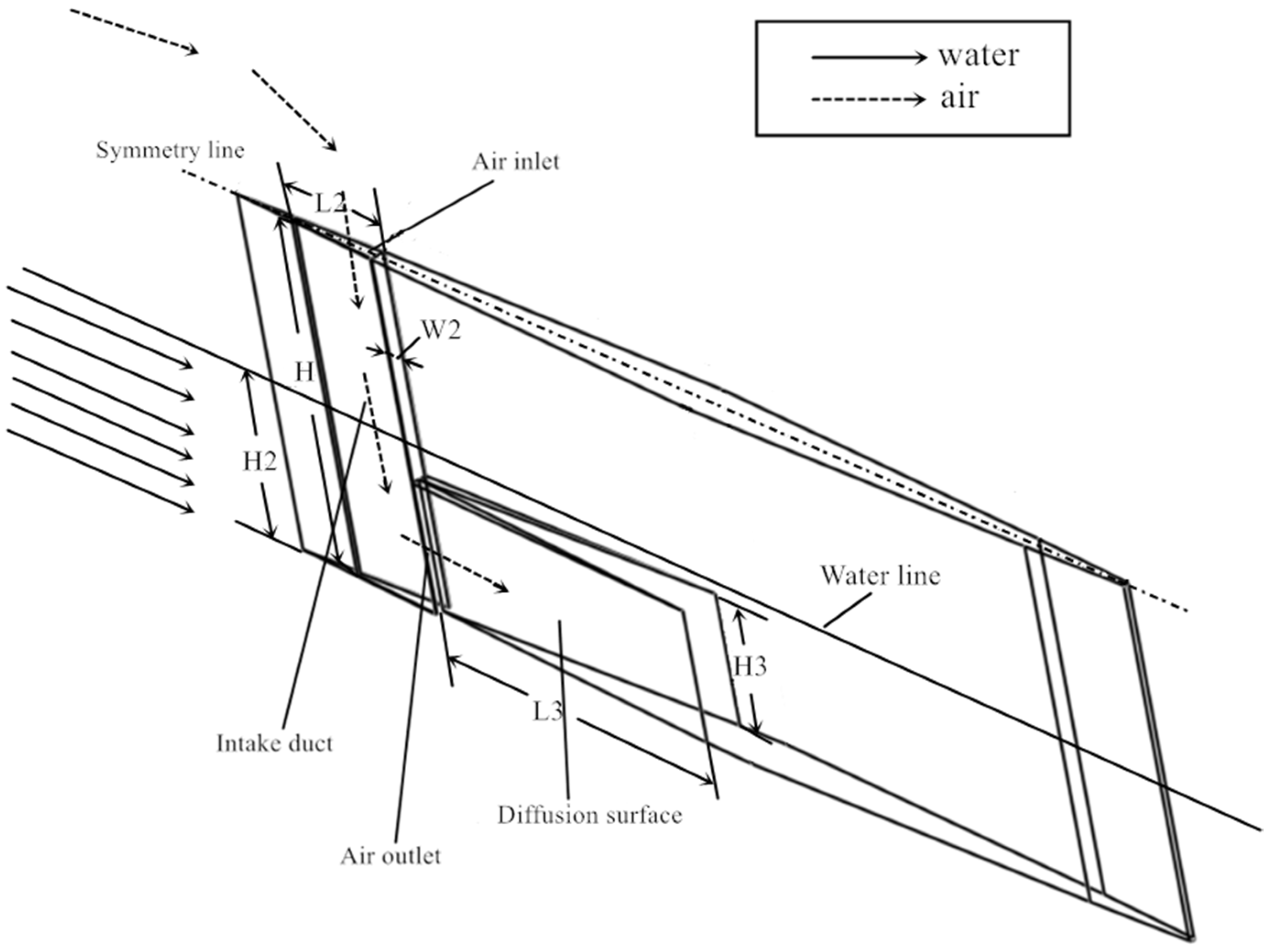
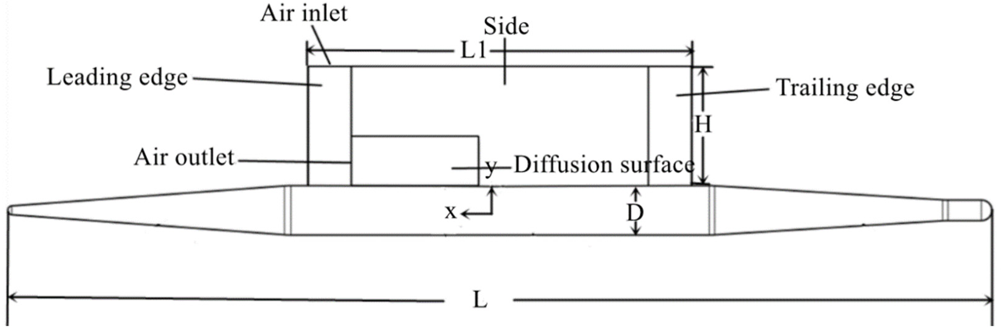
2. Description of the Physical Model

The Venturi effect is defined as the flow through the cross-section of the passage, where the flow velocity increases continuously. The flow velocity is inversely proportional to the passage cross-section. Moreover, Bernoulli’s law indicates that the increment in the flow velocity is accompanied by a decrease in the fluid pressure. Therefore, when the fluid flows through a nozzle with an expanding cross-section, the pressure of the trailing edge is lower than that of the incoming flow. Figure 1 displays the process of the strut’s automatic air intake. In Figure 1, the strut of the SWATH vessel is a longitudinal symmetrical structure. An intake duct is designed on the strut. The opening at one end of the intake duct is connected to the surrounding atmosphere, while that at the other end is below the waterline. During the vehicle sailing, since the pressure at the opening below the waterline is lower than the external atmospheric pressure, the automatic air intake can be realized based on the Venturi effect. The implementation of Venturi effect in the design scheme can be theoretically verified in the following.

Figure 2 shows the planform of the strut’s automatic air intake. As can be seen from Figure 2, the bubbly flows form on the strut surface in the state of the strut’s automatic air intake when the vehicle is moving at high speed. Consider the portion from the leading edge to the air outlet of the strut as the control body, as shown in Figure 3. In the control body of Figure 3, water flows through the control plane ${\sum }_1$ and the control plane ${\sum }_2$. The Bernoulli equation is established as follows:

$$Z_1+\frac{p_1}{\rho g}+\frac{v_1^2}{2g}=Z_2+\frac{p_2}{\rho g}+\frac{v_2^2}{2g}$$

(1)

where $p_1$ and $p_2$ are the pressure of the control plane ${\sum }_1$ and the control plane ${\sum }_2$, respectively; $Z_1$ and $Z_2$ are the depth of the control plane ${\sum }_1$ and the control plane ${\sum }_2$, respectively; $v_1$ and $v_2$ are the velocity of the control plane ${\sum }_1$ and the control plane ${\sum }_2$, respectively; $\rho$ is the density of water and $g$ is acceleration of gravity.

Considering the equal depths of control planes ${\sum }_1$ and ${\sum }_2$ and the continuity of the fluid, it can be obtained that

$$\{\begin{array}{l}{Z}_1=Z_2\\ v_1{A}_{{\sum }_1}=v_2{A}_{{\sum }_2}.\end{array}$$

(2)

where $A_{{\sum }_1}$ and $A_{{\sum }_2}$ are the area of the control plane ${\sum }_1$ and the control plane ${\sum }_2$, respectively.

Substituting Equation (2) into Equation (1), it can be obtained that

$$p_2=p_1+\frac{\rho v_1^2}{2}\left[1-{(\frac{A_{{\sum }_1}}{A_{{\sum }_2}})}^2\right]<p_1$$

(3)

According to Equation (3), the pressure at the expansion control plane ${\sum }_2$ is lower than that at the control plane ${\sum }_1$ of the incoming flow. In the design of this paper, the end of the control plane ${\sum }_2$ is connected with the external atmosphere through an intake duct. When the vehicle reaches a certain speed, once the pressure $p_2$ of the control plane ${\sum }_2$ is lower than atmospheric pressure, automatic air intake can be realized.

Because of the longitudinal symmetry of the SWATH vessel’s struts, the bubbly flows that form on the surface of the struts are also symmetrical during navigation. Adopting a two-dimensional single-chip connection strut model provides a better understanding as well as simpler analytical and numerical solutions for studying ALDR of the struts.

Figure 4 shows the layout of the strut in the proposed model. As can be seen from Figure 4, the proposed model consists of the strut and the submerged vehicle. A groove is designed in the underwater part of the rear side of the leading edge of the strut. The process of the strut’s automatic air intake is shown in Figure 1. When the vehicle moves, a low-pressure zone appears in the section with the groove, and the air outlet of the intake duct is placed in this low-pressure zone. The air inlet of the intake duct is designed on the top of the strut and connected to the external atmosphere. In this case, due to the Venturi effect, the external air is blended with the incoming flow through the air outlet of the intake duct. Moreover, the resultant air–water mixture propagates backwards along the diffusion surface, covering the underwater surface of the strut and having the effect of drag reduction by bubbly flows.

The structural dimensions of the proposed model are L = 2320 mm, L₁ = 1000 mm, L₂ = 90 mm, L₃ = 300 mm, H₂ = 290 mm, H = 140 mm, H₃ = 120 mm, D = 120 mm and W₂ = 10 mm.

In order to evaluate the drag reduction effect of the proposed model, a control model is designed for comparison. The appearance and the dimension of the control model are consistent with those of the proposed model. The only difference between these two models is that the intake duct and the diffusion surface are absent in the control model so that the leading edge is smoothly joined to the side surface.

3. Numerical Model

3.1. Basic Governing Equation

Both water and air phases are treated as incompressible fluids, and the continuity of stress is implemented at the interface. According to the homogenous equalized multi-phase theory, the continuity equation and the momentum conservation equation of the mixed media can be written as follows [25]:

$$\frac{\partial {\rho }_m}{\partial t}+\frac{\partial }{\partial x_i}({\rho }_m{u}_i)=0.$$

(4)

$$\frac{\partial }{\partial t}({\rho }_m{u}_j)+\frac{\partial }{\partial x_i}({\rho }_m{u}_i{u}_j)=-\frac{\partial p}{\partial x_j}+{\rho }_m{g}_{}+\frac{\partial }{\partial x_i}\left[({\mu }_m+{\mu }_t)\left(\frac{\partial u_i}{\partial x_j}+\frac{\partial u_j}{\partial x_i}\right)\right]$$

(5)

where t is time; p is pressure; g is acceleration of gravity; $u_i$ is the velocity component and ${\rho }_m$ and ${\mu }_m$ are the density and the dynamic viscosity of the mixed media, respectively. They can be obtained by weighted averaging the volume components as follows:

$${\rho }_m={\alpha }_l{\rho }_l+{\alpha }_g{\rho }_g, {\mu }_m={\alpha }_l{\mu }_l+{\alpha }_g{\mu }_g$$

(6)

where ${\mu }_t$ is the dynamic viscosity of turbulent flow, ${\rho }_l$ is the liquid density, ${\rho }_g$ is the gas density, ${\alpha }_l$ is the liquid fraction, ${\alpha }_g$ is the gas volume fraction, ${\mu }_l$ is the liquid dynamic viscosity and ${\mu }_g$ is the gas dynamic viscosity.

The volume components of various phases should satisfy:

$${\alpha }_l+{\alpha }_g=1$$

(7)

In this study, numerical simulation is performed on both the bubbly flows covering the surface of struts and the wave-making when the strut of the vehicle passes through the water surface. While the VOF model [26] is suitable for solving the motion rules of the multiphase intersection interface, when the air flow ratio is high, it is suitable for ALDR [22]. Therefore, the VOF model is selected for conducting numerical simulation on the change observed in the bubbly flows’ formation.

In the VOF model, the method of tracing the inter-phase boundary is achieved by solving the volume fraction continuity equation. As for the qth phase, the volume fraction equation is [26]:

$$\begin{array}{cc}& \frac{\partial {\alpha }_q}{\partial t}\end{array}+\frac{\partial }{\partial x_i}({\alpha }_q{u}_i)=0.$$

(8)

where the subscript $q=l,g$ denotes the liquid phase and the gas phase, respectively.

In addition, due to the speed (≤14 m/s) of the proposed model in the study, although there is local low pressure in the outlet area of the air intake duct, the pressure is not enough to vaporize water, so the natural cavitation phenomenon is ignored.

3.2. Turbulence Model

It should be emphasized that for high air flow rate, a stable air layer is formed on the solid surface, whereas, in the case of low air flow rate, the air layer breaks up and ALDR is not achieved [27]. Due to the sailing speed (≥5 m/s) of the proposed model in this study during the automatic air intake of the strut, the pressure difference between the air outlet and the air inlet of the intake duct is enough to ensure high air flow rate, so the air volume fraction of the formed bubbly flows is above 60%. Therefore, it can be considered that drag reduction by bubbly flows adopted in this study conforms to the ALDR model.

In handling turbulent bubbly flows, the SST $k-\omega$ model developed by Menter [28] is employed in the present study. The SST $k-\omega$ model is the combination of the $k-\epsilon$ and $k-\omega$ models, which eliminates errors arising from the empirical wall function and thus provides high simulation precision for the ALDR model [22].

The turbulent kinetic energy and the specific dissipation rate can be calculated by [28]:

$$\frac{\partial (\rho k)}{\partial t}+\frac{\partial }{\partial x_j}(\rho k{u}_j)={\tau }_{ij}\frac{\partial u_i}{\partial x_j}-{\beta }^{\ast }\rho k\omega +\frac{\partial }{\partial x_j}\left[\left(\mu +\frac{{\mu }_t}{{\sigma }_{k3}}\right)\frac{\partial k}{\partial x_j}\right]$$

(9)

$$\frac{\partial (\rho \omega )}{\partial t}+\frac{\partial (\rho \omega u_j)}{\partial x_j}=\frac{\omega }{k}({\alpha }_3{\tau }_{ij}\frac{\partial u_i}{\partial x_j})-{\beta }_3\rho {\omega }^2+\frac{\partial }{\partial x_j}\left[\left(\mu +\frac{{\mu }_t}{{\sigma }_{\omega 3}}\right)\frac{\partial \omega }{\partial x_j}\right]+2(1-F_1)\frac{\rho }{{\sigma }_{{\omega }_2}\omega }\frac{\partial k}{\partial x_j}\frac{\partial \omega }{\partial x_j}$$

(10)

$${\tau }_{ij}={\mu }_t(2s_{ij}-\frac{2}{3}\frac{\partial u_k}{\partial x_k}{\delta }_{ij})-\frac{2}{3}\rho k{\delta }_{ij}.$$

(11)

$$s_{ij}=\frac{1}{2}(\frac{\partial u_i}{\partial x_j}+\frac{\partial u_j}{\partial x_i}).$$

(12)

where the model parameters such as ${\alpha }_3$, ${\beta }_3$, ${\sigma }_{k3}$ and ${\sigma }_{\omega 3}$ are the linear combinations of the corresponding coefficients in $k-\omega$ and the modified $k-\epsilon$ turbulence model as follows:

$$\mathsf{\psi }=F_1{\mathsf{\psi }}_{k\omega }+(1-F_1){\mathsf{\psi }}_{k\epsilon }, {\alpha }_3=F_1{\alpha }_1+(1-F_1){\alpha }_2.$$

(13)

$$k-\omega : {\alpha }_1=5/9, {\beta }_1=3/40, {\sigma }_{k1}=2, {\sigma }_{\omega 1}=2, {\beta }^{\ast }=9/100$$

(14)

$$k-\epsilon : {\alpha }_2=0.44, {\beta }_2=0.0828, {\sigma }_{k2}=1, {\sigma }_{\omega 2}=1/0.856, C_{\mu }=0.09$$

(15)

${\mu }_t$ is the vortex viscosity, which can be described as:

$${\mu }_t=\rho \frac{k}{\max (\omega ,S{F}_2)}$$

(16)

where S is the invariant measure of the strain rate and the values of the above coefficients come from [29]:

$$\{\begin{array}{l}{F}_1=\tanh ({\Gamma }^4)\\ \Gamma =\min (\max (\frac{\sqrt{k}}{{\beta }^{\ast }\omega y};\frac{500\nu }{\omega y^2});\frac{4\rho {\sigma }_{\omega 2}k}{C{D}_{k\omega }{y}^2})\\ C{D}_{k\omega }=\max \left(2\rho {\sigma }_{\omega 2}\frac{1}{\omega }\frac{\partial k}{\partial xj}\frac{\partial \omega }{\partial xj},{10}^{-20}\right)\\ F_2=\tanh ({\Gamma }_2^2)\\ {\Gamma }_2=\max (\frac{2\sqrt{k}}{{\beta }^{\ast }\omega y},\frac{500v}{\omega y^2})\end{array}$$

(17)

where $y$ is the distance to the nearest wall.

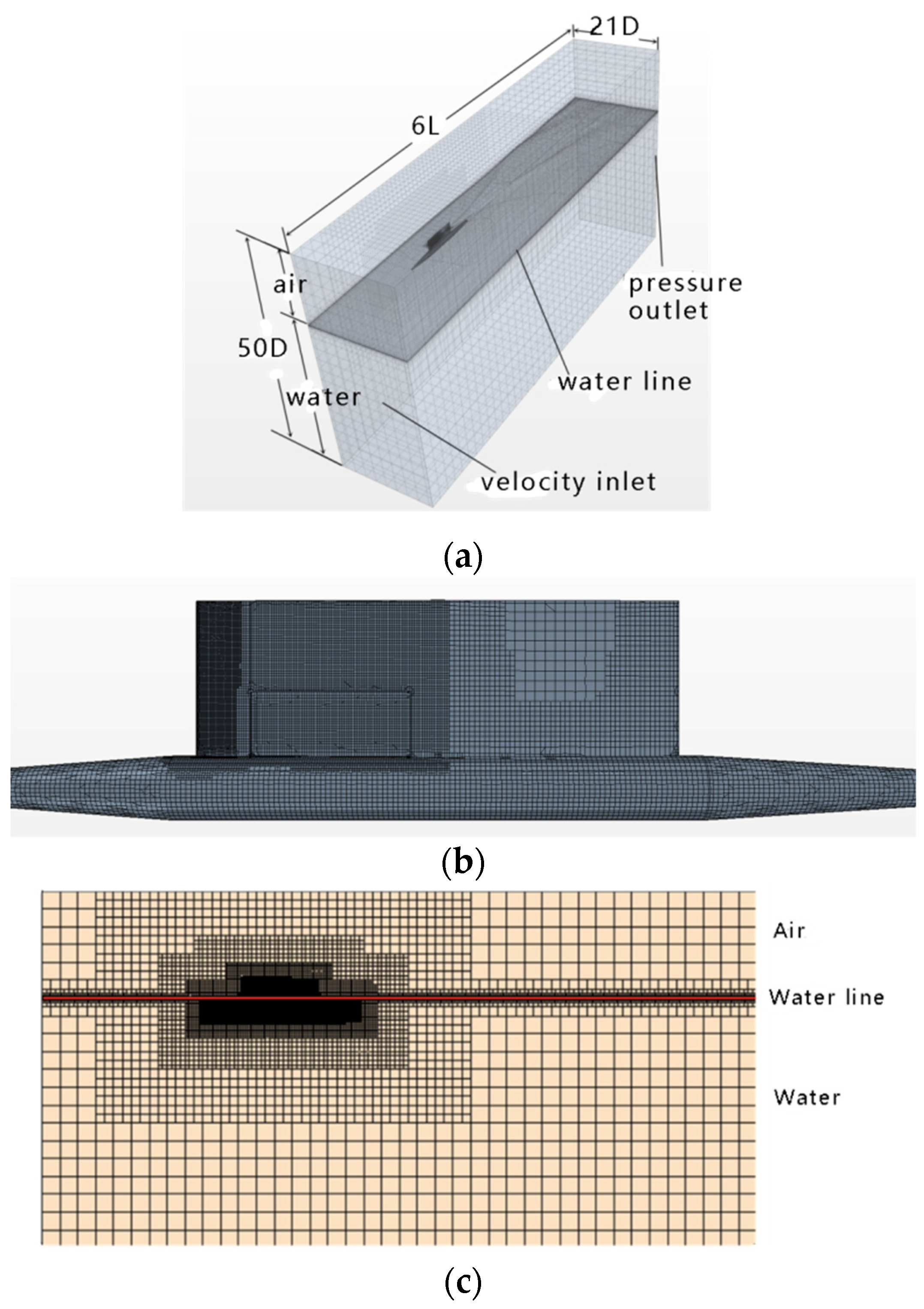
3.3. Computational Domain and Boundary Conditions

The study uses STAR-CCM+, a commercial computational fluid dynamics (CFD) software. The computing domain and boundary conditions are shown in Figure 5. Figure 5a displays the computational domain and the related grid division. The cross-sectional area is 50D × 21D and the length is 6 L. The inlet and outlet of the computational domain are defined as the velocity inlet and pressure outlet, respectively. The velocity inlet is 1.2 L away from the head of the vehicle, and the pressure outlet is located 3.8 L away from the tail of the vehicle. Parameter settings of the solver are shown in

Table 1. Parameter settings of the solver.

Parameter	Inlet Velocity (m/s)	Outlet Pressure (Pa)	Turbulence Intensity	Time Step (s)	Basic Pressure (Pa)
Setting value	5–14	Hydrostatic Pressure	0.01	0.0004	101,325

.

As part of the vehicle’s strut is above the water surface, the influence of the water surface cannot be ignored. An appropriate two-phase flow region is created in STAR-CCM+ based on the VOF model. The upper and lower halves of the velocity inlet are air and water, respectively. The inlet pressure and the outlet pressure vary in accordance with the water depth variation rule $p={\rho }_{l}gh$. A no-slip wall surface boundary condition is adopted for the wall of the vehicle. The grids on the wall surface of the vehicle are refined in Figure 5b, and mesh refinement is applied along the water-depth direction at the air–water multi-phase flow interface, as shown in Figure 5c.

3.4. Evaluation of Mesh Independence

The grid quality has an important influence on the calculation results, and the results will be more accurate if the grids are refined. In this study, three different sets of meshes with different sizes (namely, fine, moderate and coarse meshes) are generated on the surface of the control model for further mesh convergence analysis. By varying the basic mesh size, the time step is calculated, and the Courant number remains unchanged.

Table 2. Mesh parameters.

Mesh Generation	Meshing Size (mm)	Grid Number (×104)	Time Step (s)	Courant Number
$\mathrm{Fine} \mathrm{mesh} (S_1$)	3.2	140	0.0004	1
$\mathrm{Moderate} \mathrm{mesh} (S_2$)	4.8	90	0.0006	1
$\mathrm{Coarse} \mathrm{mesh} (S_3$)	6.4	50	0.0008	1

lists the detailed mesh parameters.

Under different grid conditions, the strut drag of the control model is calculated at the sailing speed of 8 m/s.

Table 3. Drag simulation results for the control model.

Mesh Conditions	$S_1$	$S_2$	$S_3$
Strut Drag (N)	43.56	44.98	51.02

lists simulation results under different mesh conditions.

The mesh independence analysis results can be calculated [2] and listed in

Table 4. Mesh independence analysis results.

Analysis Parameter	$R_k$	$C_k$	${\delta }_{k1}^{\ast }$ (%)	$U_k$ (%)	$U_{kC}$ (%)	$S_C$
Convergence	0.235	3.247	3.3%	5.5%	2.3%	44.98

. It can thus be concluded that when mesh $S_1$ is adopted, $0<R_k<1$ and the monotone convergence condition is satisfied. The error of the strut drag of the control model is 3.3%. According to mesh independence analysis results, fine mesh ($S_1$) is used in the numerical simulation.

4. Simulation Results and Analysis

4.1. Analysis of the Air Inflow Amount of the Strut Intake Duct

Since the sailing speed of the SWATH vessel in actual conditions is usually below 80 kn and considering the scale ratio of the model to be 1:9, the speed of the proposed model is set to be in the range of 1–14 m/s in the working conditions.

Table 5. Air inflow amount for different sailing speeds.

Sailing Speed (m/s)	1–4	5	6	7	8	9	10	12	14
Air Inflow Amount (kg/h)	0	5.58	9.25	12.47	14.51	16.60	19.91	29.52	38.66

presents the air inflow amount of the outlet of the intake duct for each working condition.

It is observed from Table 5 that when the sailing speed is 1–4 m/s the air inflow amount is 0. The reason for this is that at a lower sailing speed, the pressure difference between the outlet and the inlet of the duct induced by the Venturi effect is insufficient to overcome the hydrostatic pressure at the outlet as well as the pressure loss caused by the frictional drag when the air flows through the duct, with no air flowing out. However, when the sailing speed is above 4 m/s, the pressure difference between the outlet and the inlet of the duct can overcome the above-mentioned pressure loss. Therefore, the air starts flowing through the outlet of the duct. It should be indicated that higher sailing speed results in greater pressure difference and consequently more air inflow. Figure 6 illustrates the correlation between the air inflow amount and sailing speeds according to the data in Table 5. As can be seen from Figure 6, it is observed that the air inflow amount of the intake duct has a positive linear correlation with sailing speeds. Therefore, by adjusting the dimensions of the leading edge of the strut and appropriately designing the width of the intake duct, the optimal intake amount is obtained to realize the maximization of the strut drag reduction.

4.2. Analysis for the Volume Content of Air on the Surface of the Strut

As the sailing speed changes, the varying intake amount of the intake duct of the strut leads to a variable air volume fraction in the bubbly flows covering the underwater strut surface. The air volume fraction cloud diagram of the bubbly flows on the surface of the strut of the proposed model at different sailing speeds is shown in Figure 7.

It is found from Figure 7a–h that the external air is inhaled by the intake duct and blended with the incoming flow, and the resultant bubbly flows cover the underwater strut surface. The air volume fraction of the formed bubbly flows in the front of the strut is relatively higher. However, around the medium and the rear of the strut, the air volume fraction gradually declines as the inhaled air is persistently blended with water. As the sailing speed increases, the air amount of the intake duct suction increases and the air volume fraction of the formed bubbly flows increases gradually. When the sailing speed reaches 10 m/s, the air volume fraction of the bubbly flows around the front of the strut in Figure 7f is close to 1. As the speed increases further, the air volume fraction of the bubbly flows on the entire strut surface in Figure 7h is close to 1. Then, the covering effect on the strut is at its strongest.

Meanwhile, Figure 7a–h show that as the sailing speed increases, the wave-making is extended. It should be indicated that the part between the red part and the waterline in Figure 7 is the wave-making. It is worth noting that at a lower sailing speed, the wave-making is small. In Figure 7a, the wave-making above the waterline has a relatively considerable distance from the top of the strut. Therefore, the wet area of the strut above the waterline is relatively limited. As the sailing speed increases, the wave-making continuously increases. When the sailing speed reaches 14 m/s, the wave-making is considerable, and the wave-making above the waterline in Figure 7h almost reaches the top of the strut so that the part of the strut above the waterline is mostly wet.

4.3. Analysis for the Strut Drag

In this section, in order to evaluate the effect of drag reduction of the proposed model, comparative analysis is conducted on strut drags of the control model and the proposed model at different sailing speeds.

Table 6. Strut drags at different sailing speeds.

Sailing Speed (m/s)	Model Type	Strut Drag (N)	Drag Reduction Rate (%)
1	Control model	0.60	−20.00
	Proposed model	0.72
2	Control model	3.35	−9.25
	Proposed model	3.66
3	Control model	6.79	−7.51
	Proposed model	7.30
4	Control model	11.67	−2.66
	Proposed model	11.98
5	Control model	17.36	17.22
	Proposed model	14.37
6	Control model	24.16	22.10
	Proposed model	18.82
7	Control model	33.03	25.95
	Proposed model	24.46
8	Control model	43.56	28.21
	Proposed model	31.27
9	Control model	56.30	28.29
	Proposed model	40.37
10	Control model	70.47	28.03
	Proposed model	50.72
12	Control model	104.79	26.95
	Proposed model	76.55
14	Control model	144.55	25.94
	Proposed model	107.05

presents the strut drags at different sailing speeds.

It is observed from Table 4 that when the sailing speed is 1–4 m/s, the strut structure of the proposed model does not only reduce the drag but also enhances the drag. This is because, on one hand, the intake duct does not inhale air and the bubbly flows are not formed on the strut surface. On the other hand, the design of the duct and diffusion surface in the proposed model extend the wet surface of the strut in comparison to the appearance of the control model so that the frictional drag is increased. When the sailing speed is above 4 m/s, the intake duct initiates inhaling air and the bubbly flows are formed on the surface of the strut. The existence of the bubbly flows leads to reduction in the frictional drag. Moreover, as the speed increases, the air content in the bubbly flows and the drag reduction rate gradually increases. When the speed is 9 m/s, the drag reduction rate reaches its maximum at 28.29%. Figure 8 shows the variation of the drag reduction rate of the strut at different sailing speeds according to the data in Table 6.

It is observed from Figure 8 that before the sailing speed reaches 9 m/s, the drag reduction rate tends to rise linearly. However, it gradually declines when the speed reaches 9 m/s. This is because, as can be seen in Figure 5, although the increment of the air content in the bubbly flows causes the frictional drag of the strut to gradually decline as the sailing speed increases, the drag of the wave-making of the strut gradually rises. When the sailing speed is below 8 m/s, the drag reduced by formation of the bubbly flows is greater than the drag caused by the wave-making, and the drag reduction rate of the strut gradually grows. When the sailing speed reaches 8–9 m/s, the drag reduced by the bubbly flows is balanced with the drag caused by the wave-making, so the drag reduction rate of the strut remains constant. When the sailing speed is greater than 9 m/s, the drag reduced by the bubbly flows is lower than the drag caused by the wave-making. Therefore, the drag reduction rate of the strut gradually declines as the speed increases. It should be indicated that the strut drag reduction structure should be designed according to the range of the SWATH vessel speeds to achieve the best drag reduction effect.

5. Conclusions

A novel drag reduction approach to an automatic air intake strut structure is proposed in the present study. Based on the Venturi effect, a drag reduction strut structure for the SWATH vessel is designed, and a numerical study is carried out to investigate the variation of the air inflow amount, the air volume fraction in the bubbly flows and the drag reduction rate of the strut for different sailing speeds. Through analysis, the following conclusions are drawn:

(1)

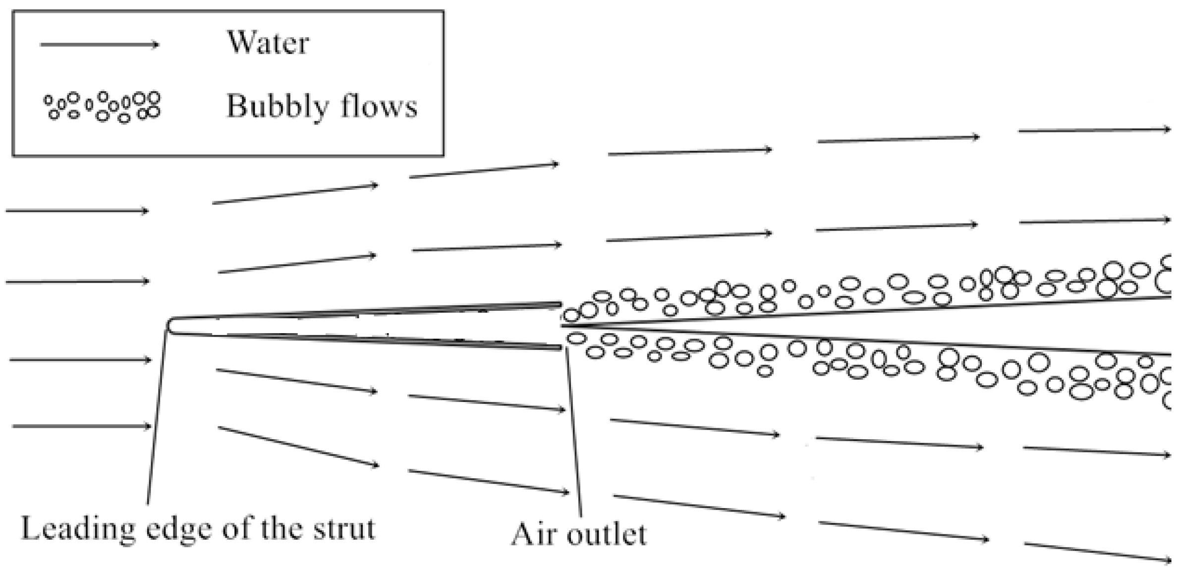
As the sailing speed increases, the external air flows through the air outlet of the intake duct and it is blended with the incoming flow, forming bubbly flows on the surface of the strut and reducing the frictional drag of the strut.

(2)

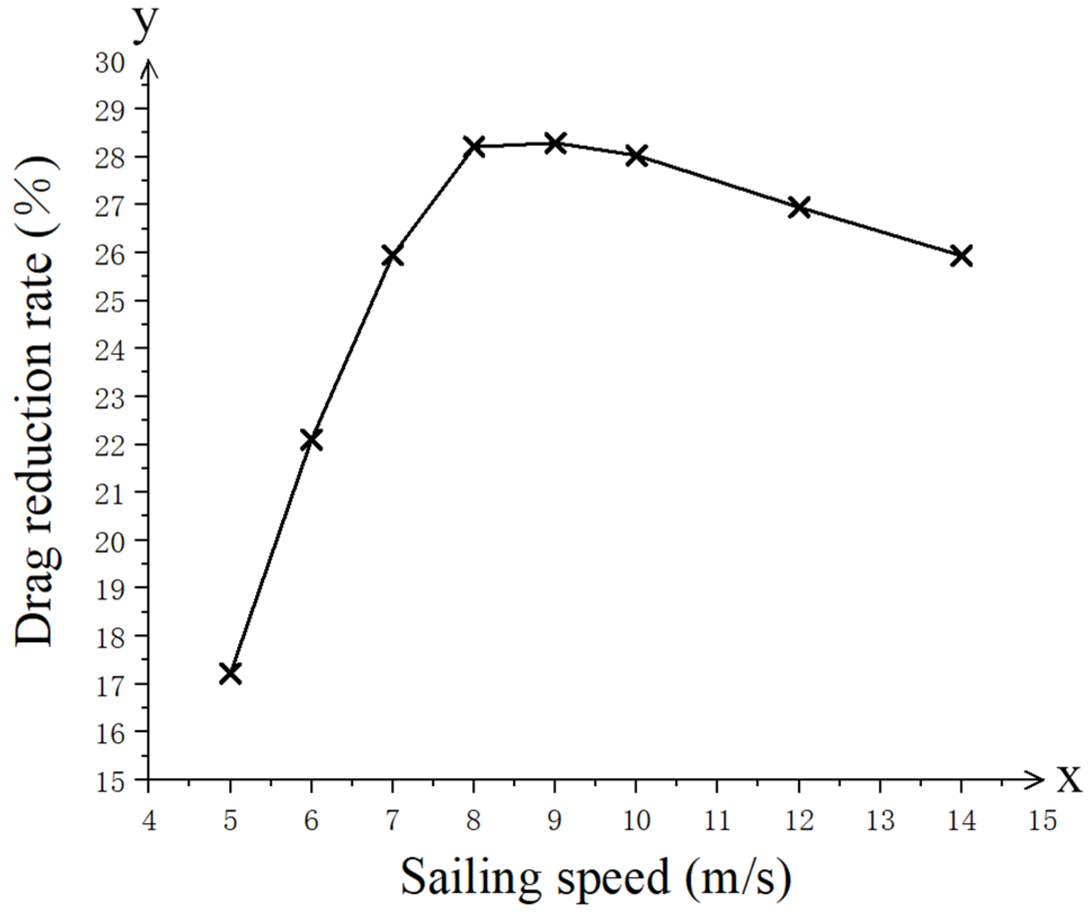
The air volume content of the bubbly flows on the surface of the strut increases as the sailing speed increases, which leads to the continuous increment of the drag reduction rate of the strut. The maximum drag reduction rate can reach about 30%, demonstrating a favorable drag reduction effect.

(3)

As the sailing speed increases, the drag of the wave-making of the strut gradually increases. When a certain speed range is reached, the drag reduces due to the formation of bubbly flows being gradually balanced with the drag caused by the wave-making, and the drag reduction rate does not increase anymore. Further increment of the speed results in a gradual decrease in the drag reduction rate.

Compared with the existing drag reduction approaches by injecting air, the proposed scheme is based on the Venturi effect with the utilization of the pressure difference between the air outlet and the air inlet of the intake duct to inhale air, not requiring artificial ventilation, which saves considerable energy and demonstrates a favorable drag reduction effect. In the future, we will continue to study the influence of the immersion depth and the shape of the automatic air intake strut structure on the air inflow amount and the drag reduction rate of the strut, and we will further design the test model of the drag reduction strut to carry out experimental verification. In a word, the proposed the automatic air intake drag reduction strut has good application prospects for achieving the targets of ship energy conservation and emission reduction. The approach of drag reduction by bubbly flows proposed in the present study provides a useful reference for the study of drag reduction of similar types of ships.

References

1. Begovic, E.; Bertorello, C.; Mancini, S. Hydrodynamic performances of small size SWATH craft. Brodogradnja 2015, 66, 1–22. [Google Scholar]
2. An, H.; Sun, P.; Ren, H.; Hu, Z. CFD-based numerical study on the ventilated supercavitating flow of the surface vehicle. Ocean Eng. 2020, 214, 107726. [Google Scholar] [CrossRef]
3. Mccormick, M.E.; Bhattacharyya, R. Drag reduction of a submersible hull by electrolysis. Nav. Eng. J. 1973, 85, 11–16. [Google Scholar] [CrossRef]
4. Murai, Y.; Fukuda, H.; Oishi, Y.; Kodama, Y.; Yamamoto, F. Skin friction reduction by large air bubbles in a horizontal channel flow. Int. J. Multiph. Flow 2007, 33, 147–163. [Google Scholar] [CrossRef]
5. Madavan, N.K.; Deutsch, S.; Merkle, C.L. Measurements of local skin friction in a microbubble-modified turbulent boundary layer. J. Fluid Mech. 1985, 156, 237–256. [Google Scholar] [CrossRef]
6. Kodama, Y.; Kakugawa, A.; Takahashi, T.; Kawashima, H. Experimental study on microbubbles and their applicability to ships for skin friction reduction. Int. J. Heat Fluid Flow 2000, 21, 582–588. [Google Scholar] [CrossRef]
7. Sayyaadi, H.; Nematollahi, M. Determination of optimum injection flow rate to achieve maximum micro bubble drag reduction in ships; an experimental approach. Sci. Iran. 2013, 20, 535–541. [Google Scholar]
8. Paik, B.G.; Yim, G.T.; Kim, K.Y.; Kim, K.S. The effects of microbubbles on skin friction in a turbulent boundary layer flow. Int. J. Multiph. Flow 2016, 80, 164–175. [Google Scholar] [CrossRef]
9. Kanai, A.; Miyata, H. Direct numerical simulation of wall turbulent flows with microbubbles. Int. J. Numer. Methods Fluids 2001, 35, 593–615. [Google Scholar] [CrossRef]
10. Kawamura, T.; Kodama, Y. Numerical simulation method to resolve interactions between bubbles and turbulence. Int. J. Heat Fluid Flow 2002, 23, 627–638. [Google Scholar] [CrossRef]
11. Xu, J.; Maxey, M.R.; Karniadakis, G.E. Numerical simulation of turbulent drag reduction using micro-bubbles. J. Fluid Mech. 2002, 468, 271–281. [Google Scholar] [CrossRef] [Green Version]
12. Ferrante, A.; Elghobashi, S. Reynolds number effect on drag reduction in a microbubble-laden spatially developing turbulent boundary layer. J. Fluid Mech. 2005, 543, 93–106. [Google Scholar] [CrossRef]
13. Mohanarangam, K.; Cheung, S.C.P.; Tu, J.Y.; Chen, L. Numerical simulation of micro-bubble drag reduction using population balance model. Ocean Eng. 2009, 36, 863–872. [Google Scholar] [CrossRef]
14. Feng, Y.-Y.; Hu, H.; Peng, G.-Y.; Zhou, Y. Microbubble effect on friction drag reduction in a turbulent boundary layer. Ocean Eng. 2020, 211, 107583. [Google Scholar] [CrossRef]
15. Haryanto, Y.; Waskito, K.T.; Pratama, S.Y.; Candra, B.D.; Rahmat, B.A. Comparison of Microbubble and Air Layer Injection with Porous Media for Drag Reduction on a Self-propelled Barge Ship Model. J. Mar. Sci. Appl. 2018, 17, 165–172. [Google Scholar]
16. Elbing, B.R.; Winkel, E.S.; Lay, K.A.; Dowling, D.R.; Perlin, M. Bubble-induced skin-friction drag reduction and the abrupt transition to air-layer drag reduction. J. Fluid Mech. 2008, 612, 201–236. [Google Scholar] [CrossRef]
17. Shen, X.; Ceccio, S.L.; Perlin, M. Influence of bubble size on micro-bubble drag reduction. Exp. Fluids 2006, 41, 415–424. [Google Scholar] [CrossRef]
18. Murai, Y. Frictional drag reduction by bubble injection. Exp. Fluids 2014, 55, 1773. [Google Scholar] [CrossRef]
19. Choi, J.K.; Hsiao, C.T.; Chahine, G.L. Numerical Studies on the Hydrodynamic Performance and the Startup Stability of High Speed Ship Hulls with Air Plenums and Air Tunnels. In Proceedings of the 9th International Conference on Fast Sea Transportation, FAST 2007, Shanghai, China, 23–27 September 2007; pp. 286–294. [Google Scholar]
20. Choi, J.K.; Georges, L.; Chahine, G.L. Numerical Study on the Behavior of Air Layers Used for Drag Reduction. In Proceedings of the 28th Symposium on Naval Hydrodynamics, Pasadena, CA, USA, 12–17 September 2010; pp. 1–15. [Google Scholar]
21. Kim, D.; Moin, P. Direct Numerical Study of Air Layer Drag Reduction Phenomenon Over a Backward-Facing Step; 63rd Annual Meeting of the APS Division of Fluid Dynamics; Center for Turbulence Research: Stanford, CA, USA, 2010; pp. 351–362. [Google Scholar]
22. Zhao, X.; Zong, Z.; Jiang, Y.; Sun, T. A numerical investigation of the mechanism of air-injection drag reduction. Appl. Ocean Res. 2020, 94, 101978. [Google Scholar] [CrossRef]
23. Kim, S.; Oshima, N. Numerical prediction of a large bubble behavior in wall turbulent flow. In Proceedings of the 14th World Congress in Computational Mechanics and ECCOMAS Congress 600, Paris, France, 19–24 July 2020; pp. 1–7. [Google Scholar]
24. Zhao, X.-J.; Zong, Z.; Jiang, Y.-C. Numerical study of air layer drag reduction of an axisymmetric body in oscillatory motions. J. Hydrodyn. 2021, 33, 1007–1018. [Google Scholar] [CrossRef]
25. Zhang, Y.J. The Daqo of Fluid Mechanics; Beijing University of Aeronautics and Astronautics Press: Beijing, China, 1991. (In Chinese) [Google Scholar]
26. Hirt, C.W.; Nichols, B.D. Volume of fluid (VOF) method for the dynamics of free boundaries. Comput. Phys. 1981, 39, 201–225. [Google Scholar] [CrossRef]
27. Kim, D. Direct numerical simulation of two-phase flows with application to air layer drag reduction. Ph.D. Thesis, Standford University, Stanford, CA, USA, June 2011. [Google Scholar]
28. Menter, F.R. Two-equation eddy-viscosity turbulence models for engineering applications. AIAA J. 1994, 32, 1598–1605. [Google Scholar] [CrossRef] [Green Version]
29. Pendar, M.R.; Roohi, E. Investigation of cavity around 3D hemispherical head-form body and conical cavitators using different turbulence and cavity models. Ocean Eng. 2016, 112, 287–306. [Google Scholar] [CrossRef]
Figure 1. Process of the strut’s automatic air intake.
Symmetry 14 00367 g001
Figure 2. Planform of the strut’s automatic air intake.
Symmetry 14 00367 g002
Figure 3. Control body.
Symmetry 14 00367 g003
Figure 4. Layout of the strut in the proposed model.
Symmetry 14 00367 g004
Figure 5. Computing domain and boundary conditions: (a) computation domain and grid division; (b) grids on the wall surface of the vehicle; (c) refined grids near waterline height.
Symmetry 14 00367 g005
Figure 6. Correlation between the air inflow amount and sailing speeds.
Symmetry 14 00367 g006
Figure 7. Volume Fraction of air cloud diagram of the bubbly flows on the surface of the strut at different sailing speeds: (a) at the sailing speed 5 m/s; (b) at the sailing speed 6 m/s; (c) at the sailing speed 7 m/s; (d) at the sailing speed 8 m/s; (e) at the sailing speed 9 m/s; (f) at the sailing speed 10 m/s; (g) at the sailing speed 12 m/s; (h) at the sailing speed 14 m/s.
Symmetry 14 00367 g007
Figure 8. Variation of the drag reduction rate of the strut at different sailing speeds.
Symmetry 14 00367 g008