A Systematic Multichimera Transform for Color Image Representation

Abstract

Mathematically representing an image with only a small number of coefficients has been attempted a few times. These attempts represent initial steps to achieve this goal and showed promising results by either working on a small image block size or utilizing a codebook built using a complex operation. The use of the codebook complicated the entire transformation process. In this work, we overcome these difficulties by developing a new scheme called systematic multichimera transform (SMCT). This transform employs simple mathematical functions called fractal half functions to independently build a codebook of image contents and size. These functions satisfy the symmetry under fractal form while breaking the orthogonality condition. The transform can deal with different image block sizes such as $8\times 8$, $16\times 16$, and $32\times 32$. The encoding process is conducted by repetitively finding the similarity between image blocks and codebook blocks to achieve data reduction and preserve important information. The coefficients of the matching process are then employed in the decoding process to reconstruct the image. SMCT produced the highest structural similarity index (SSIM) and a competitive Peak Signal to Noise Ratio (PSNR) over the standard discrete wavelet transform (DWT) and discrete cosine transform (DCT) without degrading important image content.

1. Introduction

The important role of multimedia information systems in various fields of human life is rapidly expanding. In applications where large amounts of spatial data are required to solve complex problems, efficient representations of data and fast transmission over various channels are required [1]. Digital images contain a huge amount of information that requires a large storage capacity and bandwidth for handling and transmitting purposes. Several image-processing methods seek efficient image representations that better encode important information using a small number of coefficients to reduce the required processing time and boost performance. These representations are essential in many applications, such as image watermarking [2,3], compression [4], pattern recognition [5], image retrieval [6], and image fusion [7]. Several transformations emerged to estimate an efficient representation of images. The use of image transformation can simplify the computation of convolution and correlation processes, remove redundant information, eliminate the correlation between image points, and provide a compact representation using a small number of coefficients [8]. The characteristics of the image transforms are varied on the basis of their basis functions. The most popular transformations used in image processing and computer vision applications are discrete Fourier transform (DFT), discrete cosine transform (DCT), discrete wavelet transform (DWT), Walsh–Hadamard transform (WHT), and Karhunen–Loeve transform (KLT) [9,10,11].

DFT [12] represents the image as a set of sine and cosine frequencies (functions). Therefore, its calculations include complex values. DCT [13] decomposes the image into a set of cosine functions. This transform is the basis for the international standard lossy image compression (JPEG) algorithm. In [14], a new scheme was implemented to reduce the computational complexity of the DCT where only a few arithmetic addition operations are utilized in its implementation over $8\times 8$ image blocks. To improve the quality of the transform, Brahimi et al. [15] implemented DCT using a small set of arithmetic addition and multiplication operations. In both previous schemes [14,15], the quality of transform is influenced by the number of coefficients retained. DWT [16,17] applies low- and high-pass filters to decompose the image into multiple subimages in multiresolution representation. As the level of decomposition increases, computational resources rise. This transform represents the core of the JPEG 2000 compression algorithm. The main limitation of this transform is that it cannot efficiently deal with image edges and corners due to the lack of anisotropic singularity support. To cope with this weakness, several other transforms are adopted, such as Curvelets, Ridgelets, Contourlets, and Shearlets [8]. WHT [18] uses a set of rectangular and square basis functions with values of $-1$ and $+1$ to decompose am image. The computation of this transform is faster than that of DFT due to the simplicity of its basis functions. Generalized Walsh–Hadamard transforms were recently proposed [19]. These transforms are built by deriving orthogonal and symmetric matrices with an exponential form. The basis functions are then extracted from these matrices and used for image representation. KLT [20] is a popular method for dimensionality reduction that is mainly based in principal component analysis (PCA). This transform seeks directions with the maximal covariance between them, such that data can be represented using a smaller number of uncorrelated variables. This type of transformation is widely used as a preprocessing step and it is data-dependent. A fast implementation of the KLT was introduced in [21], in which elements of the KLT matrix were approximated using the round function.

According to the type of application, the computational complexity of image processing operations varies. When an image is transformed to a mathematical representation, the computation complexity of image processing operations could be hugely reduced, as it would only be required to deal with the coefficients of the representation instead of image data points. However, converting the image into a mathematical representation requires a huge amount of work and multistep analysis. Some efforts were conducted in [22,23,24,25] to convert the image into a set of mathematical representations, which demonstrated the initial steps to achieve this goal. In [22], each image block was expressed as three coefficients using a new curve-fitting technique with a hyperbolic tangent function. By exploiting the symmetrical property of this function, reconstruction errors were minimized, and the quality of the reconstructed image texture was improved. A maximal peak signal-to-noise ratio (PSNR) of 20 dB was obtained when applying this method on a set of images. The main limitation of this method is that it can only deal with an image block of $4\times 4$, and its efficiency deteriorates with larger block sizes. To solve this limitation, the hyperbolic tangent function was employed after applying the DCT in [23]. This improved the quality of the reconstructed image. However, the number of functions required to represent the image was still high, and ultimately the compression ratio was modest. This method is also not flexible enough to deal with different mathematical functions. Further improvement was accomplished in [24], in which a chimera transform was introduced. The image was split into blocks of $4\times 4$ pixels, and three coefficients were then estimated from each one. To estimate these coefficients, a library of 256 masks was constructed. Masks were designed such that they represented different patterns in images. This transform achieved superior performance than that of methods in [22,23], but its performance also deteriorated when image blocks became larger than $4\times 4$. To mitigate this drawback, a multichimera transform was developed in [25]. This transform splits the image into multiple blocks of size $16\times 16$ pixels. A few coefficients are estimated from each block using a precomputed codebook of size $2096\times 16\times 16$. Thus, the image can be represented using a few coefficients, and a larger compression ratio can be obtained than those obtained in [22,23,24]. The disadvantage of this method is in the way in which the codebook is generated, where statistical mathematical representations and a set of images are required to construct the codebook, which complicates the whole work.

In this work, we introduce a new scheme to simply and independently build the codebook of image contents and dimensions. The codebook is built using only a set of binary two-dimensional (2D) functions (deterministic way) without any previously collected images. The encoding process is conducted by calculating the similarity between image blocks and codebook blocks. The encoded image is mainly constructed by estimating the coefficients of the matching block in the codebook for each image block. To minimize the search space, the dimensions of the codebook are only restricted by the size of the image block. The quality of the reconstructed image is improved by recursively implementing the matching process to preserve more image details. This scheme is called systematic multichimera transform (SMCT) and represents an extension to the work in [22,23,24,25]. Efforts are ongoing to accomplish more advanced steps towards converting an image into full mathematical representations. The contributions of the current work are as follows.

• A simple image transform is proposed based on recursively finding the similarity between a precomputed codebook and image blocks.
• A simple set of 2D functions are derived to build a codebook independently of image contents and dimensions. The size of the codebook is relatively proportional to the image block size.
• This transform supports different image block sizes, which eventually leads to obtaining different compression ratios.
• The matching process between image and codebook is directly conducted without any complex transformations or huge mathematical calculations.

This work is organized as follows: Section 2 describes the proposed transform and its main parts. Section 3 highlights the main experiments and their results. In Section 4, the main concluding points and future work are depicted.

2. Theoretical Background

2.1. Advantages of Mathematical Representation Instead of Data

In general, each image consists of scattered data that generate some difficulties on how to deal with the image in the various fields. These scattered data have a huge amount of probability, for example, a particular block in an image of size $8\times 8$ pixels has $3\times {256}^{8\times 8}$ (about $4\times {10}^{154}$) forms. Hence, if we convert this block into a binary image, it has $2^{8\times 8}$ (about $1.8\times {10}^{19}$) forms. The conversion of these scattered data (image block) into a systematic representation simplifies any procedure that is required to process a few coefficients of a systematic equation instead of scattered huge data. The main purpose of using these functions instead of the data is:

• Simplified processing: Image processing fields such as filtering, edge detection, resizing, and color conversion require working on each pixel (point in the image). As a result, a huge number of mathematical operations are required. If data are converted into some mathematical representations, this reduces the required number of operations.
• Image analysis and classification: Image analysis and classification depend on similarity between image details. This similarity is sensitive to many factors, such as resizing, rotation, noise contamination, and color changes, while the similarity between mathematical functions could be simpler, faster, and more stable in comparison with the similarity between images. For example, to remove image background, a full analytical process is required to first capture the background and then scan all points to remove the background. If the image is represented as a set of functions, the detection and removal of the background could be simpler because the modification of some coefficients in the function is expected to remove the image background. Our previous work in [25] applied the multichimera transform to image analysis and reconstruction.
• Image security: converting an image block into a mathematical representation provides autocoding for the image because an intruder cannot restore the image without having a particular function library.

2.2. Properties of the Proposed Mathematical Representation

A mathematical representation is considered as the basic form of representing the relationship between input and output. A representation is a rule that assigns an output value $f\left(x\right)$ to each input x. Such a representation could be deterministic since the output is completely determined by the input. Mapping is a special type of representation that can illustrate the relationship between two sets. To realize the ability of an efficient mathematical representation in converting an image into a set of functions, a suitable 2D function must be proposed, as is discussed in the next section. The proposed mathematical form employed to represent the image in this work satisfied the following conditions:

• Efficiency of 2D image representation: the first condition to satisfy a successful transformation; output values of the mathematical expression should be able to give a three-dimensional surface similar in topology to the original image points with small error.
• Simple form functions: Mathematical expressions or functions should be as simple and commonly used as possible; but this requirement might conflict with the first condition. To solve this conflict, an optimization process could be implemented with some skill and experience to determine the type of function depending on the basis of the transformation process, and taking into account the rest of the conditions.
• Suitability for fractals: An important goal of fractal geometry is to describe images in terms of transformations that in some way keep images unaltered. One of the most common properties of fractal geometry is the complex form that results from a simple process.
• Approval for digital: Logical operations and functions are the simplest mathematical form with the fastest implementation, and are more consistent with the computer language. The set of the 2D binary functions that are employed to represent the image in the proposed transform satisfies this condition (see Section 3.1). These functions would make the conversion process more flexible.

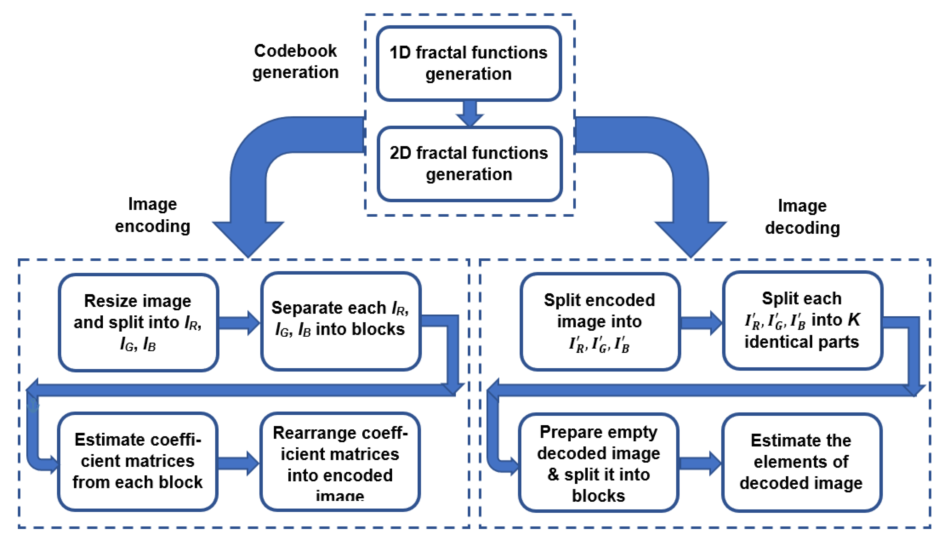
3. Systematic Multichimera Transform (SMCT)

The main structure of SMCT consists of three phases: codebook establishment, image encoding, and image decoding. The codebook establishment phase constitutes generating a set of 2D binary functions in two steps. The encoding phase mainly depends on conducting the matching process between codebook and image on a block-by-block basis. The matching process produces a set of coefficients for each block that are eventually stored in the encoded image. The decoding phase comprises reconstructing the original image from the encoded image via the codebook. These phases are demonstrated in Figure 1 and described in more detail in the following subsections.

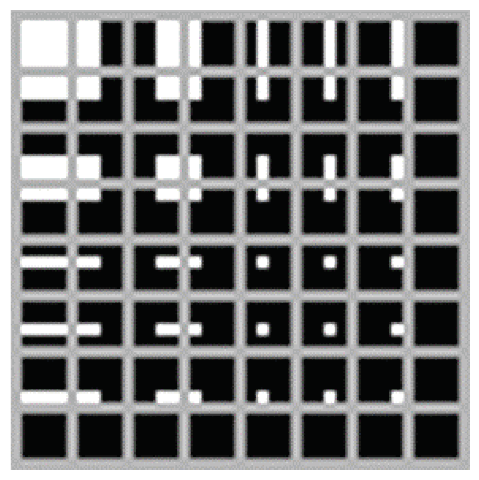
3.1. Codebook Establishment

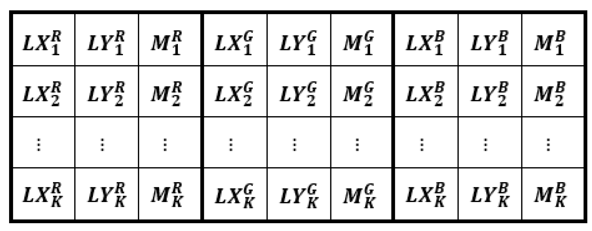
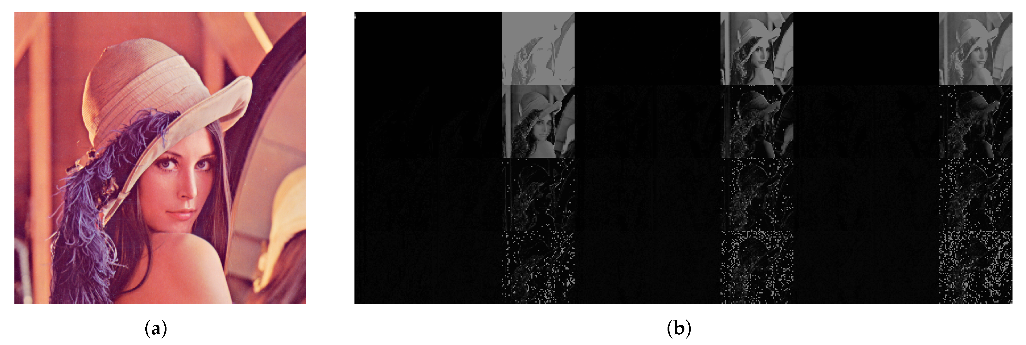
The process of codebook establishment is simple and is deterministically determined. The codebook is deterministically built by generating a set of 2D binary functions in two steps. First, a set of N one-dimensional (1D) binary functions is generated. Each of these functions has N elements. Second, a codebook is established through a set of 2D square functions with a dimension of $N\times N$. These 2D functions represent different patterns. Further details are provided below.

1D function generation: a set of 1D binary functions called fractal half functions are generated by firstly choosing a mother (basis) function ($f1$) with all its elements set to ones. This represents the first level. The functions in the second level are generated by dividing the mother function into two halves using binary step functions. A similar procedure is applied to each function in the previous level to generate the functions in the other intermediate levels. Lastly, the function at the last level is generated by setting all its elements to zeros. Figure 2 indicates the generation of the 1D functions for any N. There are N functions separated over Z levels where $Z=\left(lo{g}_{2}N\right)+1$. Except for the last level, there are $2^{Z-1}$ functions in each level where Z is the level number. For example, if we consider the value of $N=8$, a set of eight binary 1D functions is derived as follows.

$$\begin{array}{ccc}{f}_1\left(n\right)=1& \mathrm{where}& n\in \{1,2,\dots 8\}\\ f_2\left(n\right)=1& \mathrm{where}& n\in \{1,2,\dots 4\}\\ f_3\left(n\right)=1& \mathrm{where}& n\in \{5,6,\dots 8\}\\ f_4\left(n\right)=1& \mathrm{where}& n\in \{1,2\}\\ f_5\left(n\right)=1& \mathrm{where}& n\in \left\{3,4\right\}\\ f_6\left(n\right)=1& \mathrm{where}& n\in \left\{5,6\right\}\\ f_7\left(n\right)=1& \mathrm{where}& n\in \left\{7,8\right\}\\ f_8\left(n\right)=0& \mathrm{where}& n\in \left\{1,2,\dots 8\right\}\end{array}$$

(1)

These functions preserve the symmetry under fractal form in 1D but break the orthogonality condition. The value of $N\in \{8,16,32\}$ was adopted in the current work. Equations of 1D functions for $N=16$ and 32 can be similarly constructed as with N = 8.

2D functions generation: 1D functions generated in the previous step are used to construct a set of 2D functions. Each of these 2D functions represents a particular pattern that eventually forms the final codebook. The 2D functions are produced by implementing the outer product between each pair of 1D functions as demonstrated below.

$$f_{i,j}=f_i⨂f_j\mathrm{where}i,j=1,2,\dots N$$

(2)

where ⊗ stands for outer product operation, and $f_{i,j}$ is a 2D function. Consider that a and b are two vectors with length Q; the outer product between them is calculated as follows.

$$a⨂b=\left[\begin{array}{cccc}{a}_1{b}_1& a_1{b}_2& \cdots & a_1{b}_Q\\ a_2{b}_1& a_2{b}_2& \dots & a_2{b}_Q\\ ⋮& ⋮& \ddots & ⋮\\ a_Q{b}_1& a_Q{b}_2& \dots & a_Q{b}_Q\end{array}\right]$$

(3)

When the number of 1D functions is N, the number of 2D functions is $N\times N=N^2$. These 2D functions are arranged in a 2D space to obtain the codebook. Figure 3 demonstrates the representation of the codebook when N equals 8.

Each square cell in Figure 3 reflects a block of size $8\times 8$. The construction of this codebook is straightforward, which facilitates the implementation of the SMCT. The size of the codebook is related to the size of the image block and is not affected by the size of the image. As the size of the image block grows, the size of the codebook grows.

Table 1. The comparison of the DWT, DCT, and SMCT.

DWT	DCT	SMCT
Elements of its (Haar) basis functions consist of −1 and +1 only.	Elements of its basis functions are between −1 and +1.	Elements of its basis functions consist of 0 and 1.
The energy of its elements is fixed.	The energy of its elements is fixed.	The energy of its elements is decreasing.
Orthogonal	Orthogonal	Nonorthogonal
Symmetrical	Symmetrical	Symmetrical

indicates the comparison of DWT, DCT, and SMCT.

3.2. Image Encoding

The image encoding phase passes through three stages: preprocessing, matching, and postprocessing. In the preprocessing stage, the image is separated into nonoverlapping blocks. The matching stage is then calculated to repetitively find the best matching codebook block for each image block and estimate the corresponding matching coefficients. These coefficients represent the location of a matching block in the codebook for a certain image block and a normalization factor. Lastly, coefficients of the matching stage are rearranged to form the encoded image in the third stage. The transform includes two tuneable parameters (K and T), where K illustrates the number of times that the transform is implemented, and its range is $1<K<8$, while T acts as normalization parameter, and its range is $0<T<1$. The stages of the encoding phase are described in more detail in the following:

Step 1: Resize the color image to turn its size into a multiple of N, and then split the new color image into three separate images: red ($I_R$), green ($I_G$), and blue ($I_B$).

Step 2: Separate each image ($I_R$, $I_G$, and $I_B$) into nonoverlapping blocks of size $N\times N$ as

$$I_c=\{B_{1,1}^c,B_{1,2}^c,\dots B_{P,S}^c\}$$

(4)

where $c\in \{R,G,B\}$, while P and S denote the number of image blocks over the horizontal and vertical directions, respectively.

Step 3: From each block in $I_R$, $I_G$, and $I_B$, estimate three coefficient vectors $(l{x}^c,l{y}^c,m^c)$ using Steps 4–9.

Step 4: Set $B=B_{p,s}^c$ where $B_{p,s}^c$ denotes the current image block, and $(p,s)$ is the index of the image block over the vertical and horizontal directions, respectively.

Step 5: Repeat Steps 6–9 for K times.

Step 6: Find the maximal value of the block (B), and then multiply it by a constant (T) to estimate the value of m at index k as

$$m_k^c=\lfloor T\times \max (B)\rfloor$$

(5)

where $\lfloor \rfloor$ returns the largest integer. The m parameter acts as a normalization factor that facilitates the matching process between the image and the binary codebook.

Step 7: Compare the image block (B) with each block in the codebook (CB) by multiplying (CB) by $m_k^c$ and then calculating the mean absolute error (MAE) between them using

$$\left\{MA{E}_{x,y}\right\}=\mathrm{MAE}(B,m_k^c\times C{B}_{x,y})\mathrm{for}x,y=1,2,\dots N$$

(6)

where MAE between two vectors a and b of size L is given as

$$\mathrm{MAE}(a,b)=\frac{{\sum }_{l=1}^L|a_l-b_l|}{L}$$

(7)

Step 8: Find the index ($x,y$) of the CB block with the minimal MAE (i.e., the best match) to estimate the value of $L{X}^c$ and $L{Y}^c$ such that $l{x}^c$ stores the x values and $l{y}^c$ stores the y values as

$$(l{x}_k^c,l{y}_k^c)=\underset{x,y}{\mathrm{argmin}}\left\{MA{E}_{x,y}\right\}$$

(8)

Step 9: Update the values of the image block (B) as

$$B=B_{p,s}^c-m_k^c\times CB(l{x}_k^c,l{y}_k^c)$$

(9)

Step 10: Split the elements of the coefficient vectors $(l{x}^c,l{y}^c,m^c)$ estimated for all image blocks into $I_R$, $I_G$, and $I_B$, and rearrange them into separate matrices to denote the coefficients collected in a particular color channel and in a certain iteration (k), as shown in Figure 4. Each cell in this figure refers to a matrix of size ($P\times S$) pixels. More precisely, matrix $L{X}_1^R$ contains the values of $lx$ coefficients collected over all blocks in $I_R$ and at $k=1$. The remaining matrices in Figure 4 are similarly interpreted.

Steps 1 and 2 represent the preprocessing stage. Steps 3–9 represent the matching stage, and Step 10 represents the postprocessing stage. Figure 5 shows the representation of the Lenna image in the SMCT domain. In this representation, we set N = 8, T = 0.25, and K = 4. According to these settings, the algorithm was implemented four times. The representation in Figure 5b consists of three horizontal parts that belong to the representation of the red, green, and blue channels.

3.3. Image Decoding

The image decoding phase encompasses retrieving the original image from the encoded image via the codebook. The algorithm of image decoding involves the inverse operations to those used in the encoding phase. However, the decoding process is faster than the encoding process because the locations of the matching blocks in the codebook are already stored in the encoded image. Suppose that the values of K, T, and N are known by both sender and receiver; steps of reconstructing the original image from the encoded image are described below.

Step 1: Split the image vertically into three identical sections that correspond to the encoded parts of red, green, and blue channels.

Step 2: Split each section horizontally into K identical subsections that correspond to the three coefficient matrices that are estimated in each iteration k.

Step 3: Split each subsection vertically into three separate units to access the entries of each coefficient matrix $(L{X}_k^c,L{Y}_k^c,M_k^c)$ individually.

Step 4: To estimate the dimension of the original image, multiply the size of any coefficient matrix by N as

$$\left[\begin{array}{c}Z\\ V\end{array}\right]=N\times \left[\begin{array}{c}P\\ S\end{array}\right]$$

(10)

where $(Z,V)$ is the image size, N is the length of the 1D function that is used to construct the codebook, and $(P,S)$ is the size of each coefficient matrix (i.e., $L{X}_k^c$, $L{Y}_k^c$, and $M_k^c$).

Step 5: Set a new empty matrix (A) of size $(Z,V,3)$ and split it into blocks of size $N\times N$.

Step 6: Loop over the elements of the $L{X}_k^c$, $L{Y}_k^c$, and $M_k^c$ in three color channels and estimate the values of the corresponding blocks in A by multiplying the normalization factor in the M matrix by the codebook block in the index specified by the elements in the $LX$ and $LY$ matrices as

$$A_{x,y}^c=\sum _{k=1}^K{M}_k^c(xx,yy)\times CB(L{X}_k^c(xx,yy),L{Y}_k^c(xx,yy))$$

(11)

where $(xx,yy)$ is the index of the element in $L{X}_k^c,L{Y}_k^c$, and $M_k^c$ while $(x,y)$ is the index of the block in A and in a color channel c.

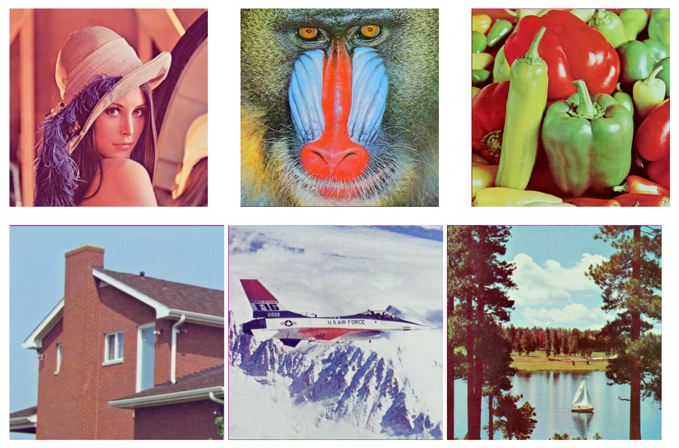
4. Experiments and Results

The effectiveness of the SMTC is demonstrated in this section. A set of analyses were conducted to show the contribution of different parameters in the proposed transform. In the experiments, the quality of the SMTC is assessed by estimating the value of the peak signal-to-noise ratio (PSNR), structural similarity index (SSIM), and the compression ratio (CR) [18,24,25]. The PSNR estimates the quality of the reconstructed (decoded) images and it is inversely proportional to the mean square error (MSE). The SSIM reflects the similarity between decoded and original images. The CR reflects the amount of information compressed by the proposed transform. Six standard color images are employed in the experiments and are presented in Figure 6. These images were Lenna, Baboon, Peppers, House, Airplane, and Lake. Each of these images had a size of $512\times 512$. Selected images had different contents and details.

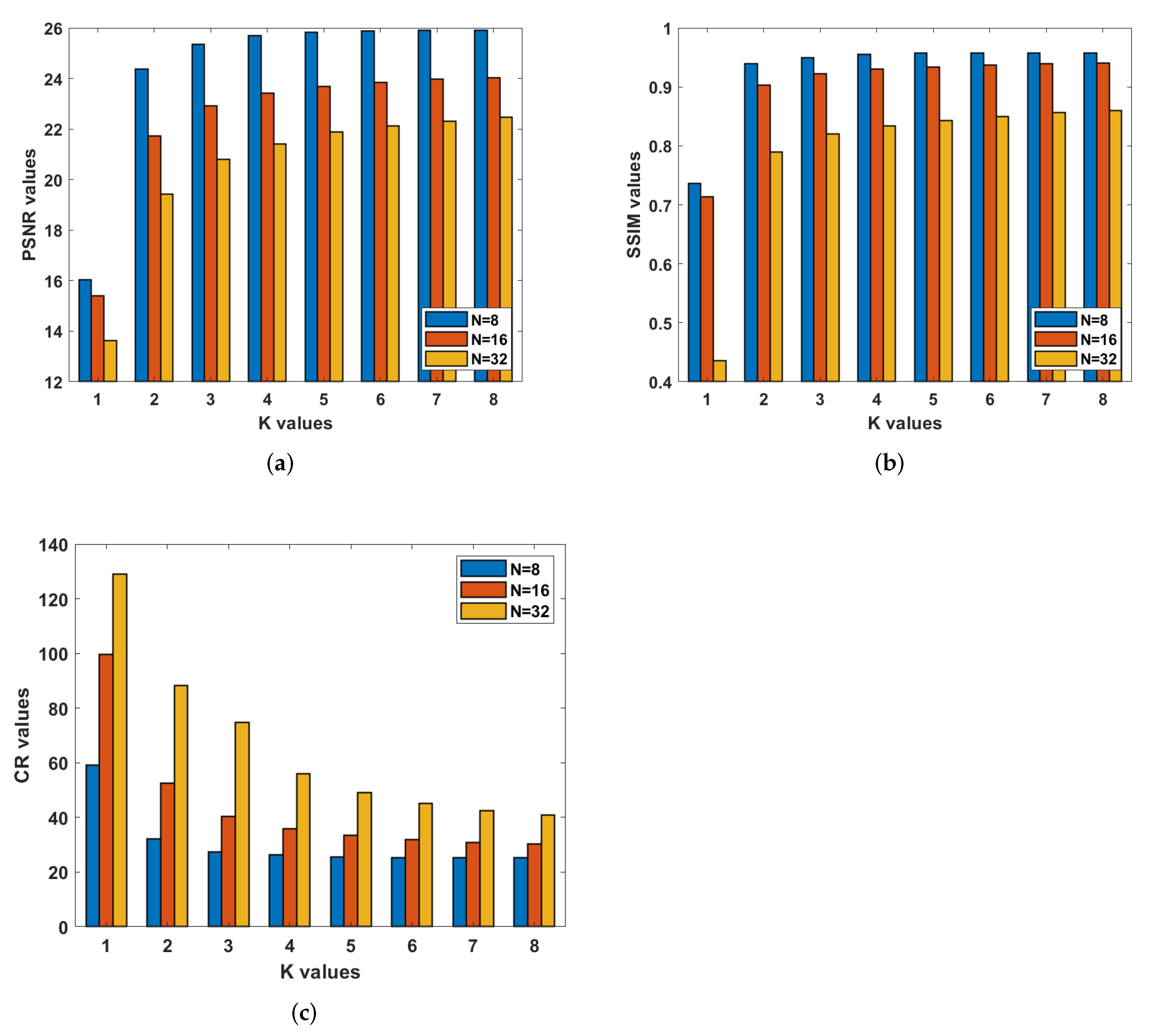
4.1. Length of Coefficient Vector (K) versus Quality and $CR$

This experiment measured the variation in the quality of the reconstructed images with the length of parameter K. To accomplish this, we applied the proposed transform on each test image by setting the values of T and N to 0.25 and 8, respectively, and modifying the number of iterations (K) required to estimate the coefficient vectors ($m^c$, $l{x}^c$, and $l{y}^c$) in Equations (6) and (8) from 1 to 8. For each K, PSNR, SSIM, and CR values are shown in

Table 2. Influence of K parameter.

Image	Quality Metric	K Parameter
		1	2	3	4	5	6	7	8
	PSNR	14.81	25.48	26.99	27.57	27.86	28	28.07	28.1
Lenna	SSIM	0.535	0.946	0.959	0.964	0.966	0.967	0.968	0.968
	CR	75.42	34.1	28.57	27.21	26.55	26.24	26.04	25.94
	PSNR	14.53	19.46	20.28	20.71	20.97	21.1	21.16	21.18
Baboon	SSIM	0.375	0.644	0.69	0.72	0.735	0.743	0.747	0.748
	CR	77.16	21.29	17.45	16.1	15.45	15.13	14.98	14.92
	PSNR	16.03	24.38	25.36	25.7	25.83	25.89	25.91	25.92
Peppers	SSIM	0.736	0.939	0.95	0.955	0.957	0.957	0.958	0.958
	CR	59.15	32.07	27.41	26.23	25.67	25.39	25.28	25.20
	PSNR	14.72	27.34	29.32	29.84	30.02	30.11	30.14	30.15
House	SSIM	0.508	0.928	0.952	0.96	0.963	0.964	0.965	0.966
	CR	105.41	40.85	34.63	32.94	31.97	31.53	31.14	30.96
	PSNR	11.38	23.37	24.68	25.1	25.27	25.35	25.38	25.39
Airplane	SSIM	0.585	0.793	0.842	0.86	0.869	0.873	0.876	0.877
	CR	105.26	40.37	30.32	28.88	28.02	27.59	27.41	27.27
	PSNR	14.12	21.93	23.09	23.59	23.81	23.92	23.96	23.97
Lake	SSIM	0.523	0.83	0.864	0.878	0.884	0.887	0.888	0.888
	CR	66.62	25.99	21.74	20.63	20.09	19.88	19.78	19.76

.

The table indicates that the quality of images improved as the number of iterations increased. The worst quality was achieved when the transform was only implemented once. Considerable improvement was achieved when we repeatedly applied the transform on the resulting images. However, the improvement in image quality was modest when the value of K was greater than 4. Image contents showed that the quality of images with a few small details (i.e., Lenna, Peppers, and House) was better than that with highly complex details (i.e., Baboon, Airplane, and Lake). On the other hand, we achieved the highest compression ratio when the value of K equaled 1. After that, it began to significantly decrease until the value of K reaches 4, and it then slightly decreased. The value of the CR was also influenced by the details of the image contents. The highest CR was recorded for the House image (a few small details), and the lowest CR was recorded for the Baboon image (many small details). To obtain a compromise between the quality of the reconstructed image and the compression ratio, the value of K should be set to 4.

4.2. Influence of Parameter T versus Quality

This experiment measures the variation of the quality of the reconstructed images with the value of the parameter T. In this experiment, we applied the proposed transform on the Lenna image by varying the value of T from 0.15 to 0.95 at a step of 0.1, and the number of iterations (K) from 1 to 8. For each pair of T and K, PSNR and SSIM values were estimated and are displayed in

Table 3. Variation in T versus K parameter.

T	Quality Metric	K Parameter
		1	2	3	4	5	6	7	8
0.15	PSNR	14.79	25.37	26.86	27.46	27.79	27.95	28.04	28.08
	SSIM	0.534	0.945	0.958	0.963	0.965	0.967	0.968	0.968
0.25	PSNR	14.81	25.48	26.99	27.57	27.86	28.00	28.07	28.10
	SSIM	0.535	0.946	0.959	0.964	0.966	0.967	0.968	0.968
0.35	PSNR	14.82	25.50	27.00	27.55	27.82	27.95	28.00	28.02
	SSIM	0.535	0.947	0.959	0.964	0.966	0.967	0.967	0.967
0.45	PSNR	14.82	25.42	26.92	27.48	27.74	27.86	27.91	27.92
	SSIM	0.535	0.947	0.959	0.964	0.965	0.966	0.967	0.967
0.55	PSNR	14.79	25.14	26.69	27.30	27.58	27.70	27.75	27.77
	SSIM	0.532	0.945	0.958	0.963	0.965	0.965	0.966	0.966
0.65	PSNR	14.72	24.54	26.21	26.99	27.33	27.48	27.55	27.57
	SSIM	0.528	0.941	0.956	0.961	0.963	0.964	0.964	0.965
0.75	PSNR	14.53	23.55	25.38	26.32	26.82	27.06	27.18	27.24
	SSIM	0.518	0.932	0.950	0.957	0.961	0.962	0.963	0.963
0.85	PSNR	14.23	22.21	24.09	25.27	25.95	26.35	26.56	26.67
	SSIM	0.502	0.917	0.940	0.951	0.956	0.958	0.960	0.960
0.95	PSNR	13.73	20.48	22.35	23.64	24.52	25.09	25.45	25.65
	SSIM	0.476	0.891	0.922	0.937	0.946	0.951	0.954	0.955

where the bold number indicates the best quality across each column.

Results show that the optimal value of T was 0.35 when values of K were from 1 to 3 (small iterations), and 0.25 when the value of K was from 4 to 8 (large iterations). However, the quality of the reconstructed image was bad for smaller values of K. Results showed the same tendency when the experiment was conducted on the other images. We, therefore, set the value of T to 0.25 in the rest of the experiments.

4.3. Parameter K versus Parameter N

We studied the relationship between parameters K and N. To accomplish this analysis, we applied the transform on all images by modifying these parameters. The value of parameter N was set to 8, 16, and 32. For each value of N, we set the value of K from 1 to 8. The relationship was estimated as shown in Figure 7 for the Peppers image in accordance to PSNR, SSIM, and CR.

This figure indicates that the quality of the reconstructed image (PSNR, SSIM) deteriorated as the value of N increased. The value of N was directly proportional to the value of K. As the value of N increased, a higher value of K was required to achieve better quality for the reconstructed image. Contrarily, CR grew when the value of N increased for all values of K. This was obvious because the same number of coefficients was estimated from each image block regardless of its size, while the total number of blocks decreased when the value of N increased, which means that more information was lost. To achieve a better compromise between image quality and the CR, the value of K can also be selected to be 4.

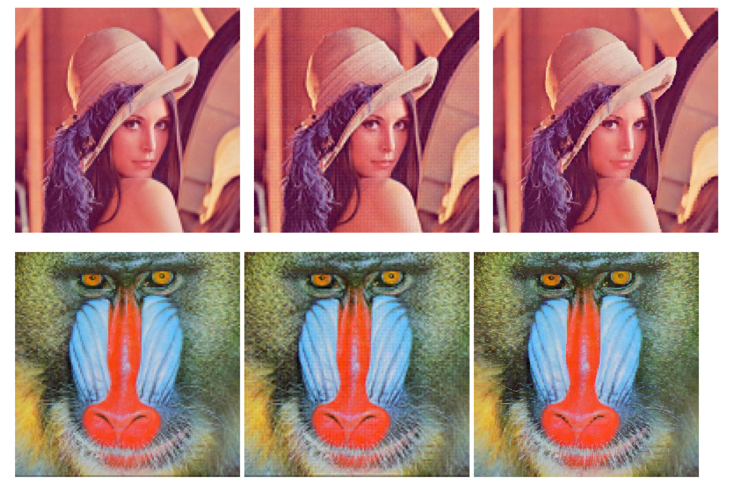
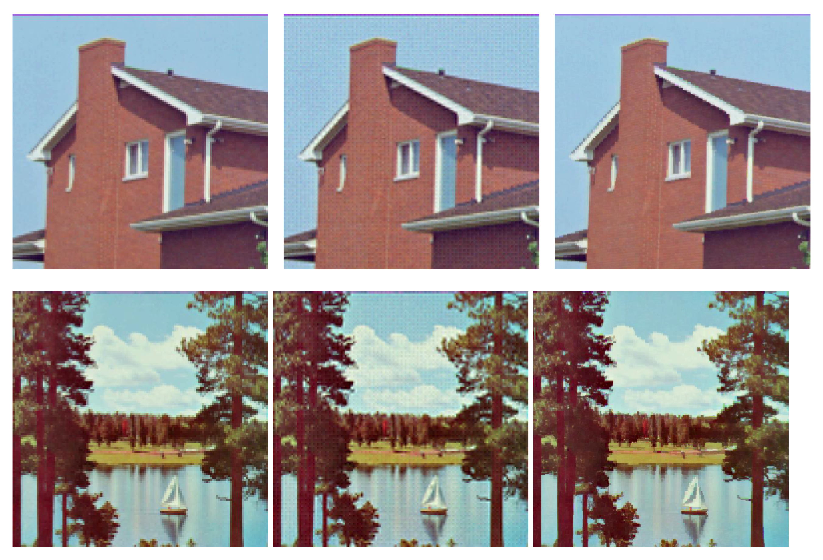
4.4. Comparison with Standard Transforms

Comparison analysis between different transforms was conducted in this experiment. The proposed transform was implemented using $N=8$, $K=4$, and $T=0.25$. Four coefficients were estimated from each block of size $8\times 8$ and used for reconstruction. To conduct a fair comparison with other transforms, we considered the same block size in DWT and DCT, and the same number of coefficients estimated from each block by setting the values of the remaining coefficients to zero. Comparison results in accordance to the PSNR and SSIM are shown in

Table 4. Comparison of different transforms.

Image	Quality Metric	Transform
		DWT	DCT	SMTC
Lenna	PSNR	26.77	27.2	27.57
	SSIM	0.954	0.955	0.964
Baboon	PSNR	20.28	20.41	20.71
	SSIM	0.655	0.657	0.720
Peppers	PSNR	25.39	26.18	25.7
	SSIM	0.946	0.953	0.955
House	PSNR	28.41	29.07	29.84
	SSIM	0.937	0.937	0.960
Airplane	PSNR	24.78	25.31	25.10
	SSIM	0.836	0.773	0.860
Lake	PSNR	23.00	23.61	23.59
	SSIM	0.849	0.852	0.878
Average	PSNR	24.77	25.29	25.41
	SSIM	0.862	0.854	0.889

using the six chosen images. Table 4 shows that SMCT outperforms other transforms as indicated by the SSIM metric for all images, and it produced comparable quality with that of other transforms as indicated by the PSNR metric. On average, the SMCT produced the highest PSNR and SSIM values.

Figure 8 shows the qualitative analysis of different transforms on four images. DCT yielded a high blocking effect on the whole reconstructed images. DWT caused a blurring effect. The SMCT had a lower blurring effect than that of DWT, while the blocking effect was only observed on the edges of the reconstructed images. These results were expected, as we only applied the transforms on images without any postprocessing operations. This aids in understanding the characteristics of this transform to formulate appropriate postprocessing operations in future work.

5. Conclusions

A new transform for image representation was developed aiming to represent an image using a small number of functions. We first built a codebook using a set of simple binary functions that aid the process of image encoding and decoding. This codebook is independent of image size and contents. The main operation in the process of image encoding is to calculate the matching process between image blocks and codebook blocks, and estimate the coefficients of the codebook block that is most similar to each image block. These coefficients were then employed to reconstruct the image from the codebook in the decoding process. Results revealed that the transform could achieve competitive performance as compared to that of DCT and DWT on six standard images in terms of PSNR and SSIM. For future work, our next efforts are to improve the quality of the reconstructed image, enlarge the size of the image block, and eliminate the need for the codebook.

References

1. Svynchuk, O.; Barabash, O.; Nikodem, J.; Kochan, R.; Laptiev, O. Image Compression Using Fractal Functions. Fractal Fract. 2021, 5, 31. [Google Scholar] [CrossRef]
2. Fares, K.; Amine, K.; Salah, E. A robust blind color image watermarking based on Fourier transform domain. Optik 2020, 208, 164562. [Google Scholar] [CrossRef]
3. Abdulsattar, F.S. Towards a high capacity coverless information hiding approach. Multimed. Tools Appl. 2021, 80, 18821–18837. [Google Scholar] [CrossRef]
4. UmaMaheswari, S.; SrinivasaRaghavan, V. Lossless medical image compression algorithm using tetrolet transformation. J. Ambient. Intell. Humaniz. Comput. 2021, 12, 4127–4135. [Google Scholar] [CrossRef]
5. Zhao, R.; An, L.; Song, D.; Li, M.; Qiao, L.; Liu, N.; Sun, H. Detection of chlorophyll fluorescence parameters of potato leaves based on continuous wavelet transform and spectral analysis. Spectrochim. Acta Part A Mol. Biomol. Spectrosc. 2021, 259, 119768. [Google Scholar] [CrossRef]
6. Khalid, M.J.; Irfan, M.; Ali, T.; Gull, M.; Draz, U.; Glowacz, A.; Sulowicz, M.; Dziechciarz, A.; AlKahtani, F.S.; Hussain, S. Integration of discrete wavelet transform, DBSCAN, and classifiers for efficient content based image retrieval. Electronics 2020, 9, 1886. [Google Scholar] [CrossRef]
7. Wang, Z.; Li, X.; Duan, H.; Zhang, X.; Wang, H. Multifocus image fusion using convolutional neural networks in the discrete wavelet transform domain. Multimed. Tools Appl. 2019, 78, 34483–34512. [Google Scholar] [CrossRef]
8. Bhuyan, M.K. Computer Vision and Image Processing: Fundamentals and Applications; CRC Press: Boca Raton, FL, USA, 2019. [Google Scholar]
9. Surówka, G.; Ogorzalek, M. Wavelet-based logistic discriminator of dermoscopy images. Expert Syst. Appl. 2021, 167, 113760. [Google Scholar] [CrossRef]
10. Begum, M.; Ferdush, J.; Uddin, M.S. A Hybrid robust watermarking system based on discrete cosine transform, discrete wavelet transform, and singular value decomposition. J. King Saud-Univ.-Comput. Inf. Sci. 2021, in press. [Google Scholar] [CrossRef]
11. Balsa, J. Comparison of Image Compressions: Analog Transformations. Proceedings 2020, 54, 37. [Google Scholar] [CrossRef]
12. Acharya, D.; Billimoria, A.; Srivastava, N.; Goel, S.; Bhardwaj, A. Emotion recognition using fourier transform and genetic programming. Appl. Acoust. 2020, 164, 107260. [Google Scholar] [CrossRef]
13. Almurib, H.A.; Kumar, T.N.; Lombardi, F. Approximate DCT image compression using inexact computing. IEEE Trans. Comput. 2017, 67, 149–159. [Google Scholar] [CrossRef]
14. Brahimi, N.; Bouden, T.; Brahimi, T.; Boubchir, L. A novel and efficient 8-point DCT approximation for image compression. Multimed. Tools Appl. 2020, 79, 7615–7631. [Google Scholar] [CrossRef]
15. Brahimi, N.; Bouden, T.; Brahimi, T.; Boubchir, L. Efficient multiplier-less parametric integer approximate transform based on 16-points DCT for image compression. Multimed. Tools Appl. 2021, 1–24. [Google Scholar] [CrossRef]
16. Geetha, V.; Anbumani, V.; Murugesan, G.; Gomathi, S. Hybrid optimal algorithm-based 2D discrete wavelet transform for image compression using fractional KCA. Multimed. Syst. 2020, 26, 687–702. [Google Scholar] [CrossRef]
17. Abdulsattar, F.S. On the Effectiveness of Using Wavelet-based LBP Features for Melanoma Recognition in Dermoscopic Images. In Proceedings of the 2021 International Conference on Information Technology (ICIT), Amman, Jordan, 14–15 July 2021; IEEE: Piscataway, NJ, USA, 2021; pp. 406–411. [Google Scholar]
18. Zheng, P.; Huang, J. Efficient encrypted images filtering and transform coding with walsh-hadamard transform and parallelization. IEEE Trans. Image Process. 2018, 27, 2541–2556. [Google Scholar] [CrossRef]
19. Dziech, A. New Orthogonal Transforms for Signal and Image Processing. Appl. Sci. 2021, 11, 7433. [Google Scholar] [CrossRef]
20. Yang, C.; Zhang, X.; An, P.; Shen, L.; Kuo, C.C.J. Blind Image Quality Assessment Based on Multi-Scale KLT. IEEE Trans. Multimed. 2020, 23, 1557–1566. [Google Scholar] [CrossRef]
21. Radünz, A.P.; Bayer, F.M.; Cintra, R.J. Low-complexity rounded KLT approximation for image compression. J. -Real-Time Image Process. 2022, 19, 173–183. [Google Scholar] [CrossRef]
22. Khalaf, W.; Zaghar, D.; Hashim, N. Enhancement of curve-fitting image compression using hyperbolic function. Symmetry 2019, 11, 291. [Google Scholar] [CrossRef] [Green Version]
23. Khalaf, W.; Al Gburi, A.; Zaghar, D. Pre and Postprocessing for JPEG to Handle Large Monochrome Images. Algorithms 2019, 12, 255. [Google Scholar] [CrossRef] [Green Version]
24. Khalaf, W.; Mohammad, A.S.; Zaghar, D. Chimera: A New Efficient Transform for High Quality Lossy Image Compression. Symmetry 2020, 12, 378. [Google Scholar] [CrossRef] [Green Version]
25. Mohammad, A.S.; Zaghar, D.; Khalaf, W. Maximizing Image Information Using Multi-Chimera Transform Applied on Face Biometric Modality. Information 2021, 12, 115. [Google Scholar] [CrossRef]
Figure 1. Block diagram of SMCT.
Symmetry 14 00516 g001
Figure 2. Generation of 1D functions for any N.
Symmetry 14 00516 g002
Figure 3. Codebook representation when N = 8.
Symmetry 14 00516 g003
Figure 4. Representation of the SMCT coefficients.
Symmetry 14 00516 g004
Figure 5. Representation of Lenna image in SMCT domain. (a) Lenna image; (b) SMCT domain.
Symmetry 14 00516 g005
Figure 6. Color images employed in the experiments.
Symmetry 14 00516 g006
Figure 7. Relationship between K and N. (a) PSNR; (b) SSIM; (c) CR.
Symmetry 14 00516 g007
Figure 8. Visual comparison of different transforms. (left) Results of applying DWT; (center) results of applying DCT; (right) results of our proposed transform.
Symmetry 14 00516 g008aSymmetry 14 00516 g008b