Formation of Fuzzy Patterns in Logical Analysis of Data Using a Multi-Criteria Genetic Algorithm

Abstract

The formation of patterns is one of the main stages in logical data analysis. Fuzzy approaches to pattern generation in logical analysis of data allow the pattern to cover not only objects of the target class, but also a certain proportion of objects of the opposite class. In this case, pattern search is an optimization problem with the maximum coverage of the target class as an objective function, and some allowed coverage of the opposite class as a constraint. We propose a more flexible and symmetric optimization model which does not impose a strict restriction on the pattern coverage of the opposite class observations. Instead, our model converts such a restriction (purity restriction) into an additional criterion. Both, coverage of the target class and the opposite class are two objective functions of the optimization problem. The search for a balance of these criteria is the essence of the proposed optimization method. We propose a modified evolutionary algorithm based on the Non-dominated Sorting Genetic Algorithm-II (NSGA-II) to solve this problem. The new algorithm uses pattern formation as an approximation of the Pareto set and considers the solution’s representation in logical analysis of data and the informativeness of patterns. We have tested our approach on two applied medical problems of classification under conditions of sample asymmetry: one class significantly dominated the other. The classification results were comparable and, in some cases, better than the results of commonly used machine learning algorithms in terms of accuracy, without losing the interpretability.

1. Introduction

Logical analysis of data (LAD) is a methodology for processing a set of observations, or objects, some of which belong to a specific subset (positive observations), and the rest does not belong to it (negative observations) [1]. These observations are described by features, generally numerical, nominal, or binary. Logical analysis of data is performed by detecting pattern-logical expressions that are true for positive (or negative) observations and not performed for negative (or, respectively, positive) observations [2]. Thus, regions in the feature space containing observations of the corresponding classes can be approximated using a set of positive and negative patterns. To identify such patterns, we use models and methods of combinatorial optimization [3,4,5].

Classification problems are one of the application fields of LAD [6,7]. From the point of view of solving classification problems, applying LAD can be considered as the construction of a rule-based classifier. Like other rule-based classification approaches, such as decision trees and lists of rules, this approach has the advantage that it constructs a “transparent” classifier. Thus, it belongs to interpretive machine learning methods.

Two types of patterns can be distinguished [8]. The first type is homogeneous (pure, clear) patterns. A homogeneous pattern covers part of the observations of a particular class (for example, positive) and does not cover any observation of another class (negative). However, if we consider real data for constructing a classifier, then pure patterns often do not give a good result. Due to the noisiness of the data, the presence of inaccuracies, errors, and outliers, pure patterns may have too low generalizing ability, and their use leads to overfitting. In such cases, the best results are shown by fuzzy (partial) patterns, in which the homogeneity constraint is weakened. Such weakening (relaxation) leads to the formation of more generalized patterns [4,9]. The pattern search problem is considered as an optimization problem, where the objective function is the number of covered observations of a certain class under a relaxed non-coverage constraint of observations of the opposite class.

Modern literature offers various approaches to the formation of patterns [8]. To generate patterns, enumeration-based algorithms [6,10], algorithms based on integer programming [2] or mixed approach based on both integer and linear programming principles [11,12] are used. In [5], a genetic algorithm for generating patterns is described. In [13], an approach based on metaheuristics is presented, in which the key idea is the construction of a pool of patterns for each given observation of the training set. Logical analysis of data is used in many application areas, such as cancer diagnosis and coronary risk prediction [2,10,11,14], credit risk rating [11,15,16,17], assessment of the potential of an economy to attract foreign direct investment [18], predicting the number of airline passengers [19], fault prognosis and anomaly detection [20,21,22,23], and others.

Thus, in traditional approaches to the logical analysis of data with homogeneous patterns, each pattern covers part of the observations of the target class and no observations of the opposite class. Otherwise, the homogeneity constraint is transformed into a relaxed non-coverage constraint related to a number or ratio of observations of the opposite class. Thus, such optimization model is not symmetric in the sense that the problem is focused on the number of covered observations of the target class while the coverage of the opposite class is considered as a constraint set at a certain level. Such an approach with the fuzzy patterns remains in the domain of the single-criterion optimization.

Recently, fuzzy logic theory has been widely developed in research. As mentioned in the literature [13], a certain degree of fuzziness seems to improve the robustness of the classification algorithm. In a fuzzy classification system, an object can be classified by applying a set of fuzzy rules based on its attributes. To build a fuzzy classification system, the most difficult task is to find a set of fuzzy rules pertaining to the specific classification problem [24]. To extract fuzzy rules, a neural net was proposed in several studies [25,26,27]. On the other hand, the decision tree induction method was used in [28,29,30]. In [30], a fuzzy decision tree approach was proposed, which can overcome the overfitting problem without pruning and can construct soft decision trees from large datasets. However, these methods were found to be suboptimal in solving certain types of problems [24]. In [13,24], a genetic algorithm for generating fuzzy rules was described. It was noted that they are very robust due to the global searching.

Fuzzy classification has practical applications in various fields. For instance, in [31], a fuzzy rule-based system for classification of diabetes was used. Authors in [32,33] have applied fuzzy theory in managing energy for electric vehicles. In [34], problems of a product processing plant related to the discovery of intrusions in a computer network were solved with use of a fuzzy classifier. In our study, we use fuzziness as a concept of partial patterns.

Both traditional and fuzzy approaches provide for finding both patterns covering the target class and patterns covering the opposite class. The methods for finding such patterns do not differ; in this sense, such approaches are symmetrical: the composition of patterns does not change from replacing the target class with the opposite one. At the same time, there is a significant difference between the requirement for maximum coverage and the requirement for purity of patterns.

When analyzing real data, pure patterns may be ineffective, and the concept of a pattern is extended to fuzzy patterns that cover some of the negative objects. This expansion occurs by relaxing the “empty intersection with negative objects” constraint. Thus, the aim of our study is to construct a classification model based on LAD principles, which does not impose a strict restriction nor relaxed constraint on the pattern coverage of the opposite class observations. Our model converts such a restriction (purity restriction) into an additional criterion. We formulate the pattern search problem as a two-criteria optimization problem: the maximum of covered observations of a certain class with the minimum of covered observations of the opposite class. Thus, our model has two competing criteria of the same scale, and the essence of solving the problem comes down to finding a balance between maximum coverage and purity of patterns. For this purpose, in this paper, we study the use of a multi-criteria genetic algorithm to search for Pareto-optimal fuzzy patterns. Our comparative results on medical test problems are not inferior to the results of commonly used machine learning algorithms in terms of accuracy.

The rest of the paper is organized as follows. In Section 2, we describe known and new methods implemented in our research. We provide the basic concepts of logical analysis of data (Section 2.1), an approach to formation of logical patterns (Section 2.2), a two-criteria optimization model for solving the pattern search problem, concepts of the evolutionary algorithm NSGA-II (Non-dominated Sorting Genetic Algorithm-II), developed to solve the multi-criteria optimization problem (Section 2.4). In Section 2.5, we discover the ability of evolutionary algorithms to solve the problem of generating logical patterns and describe modifications of the NSGA-II (Section 2.5). In Section 3, we present the results of solving two applied classification problems. In Section 4 and Section 5, we discuss and shortly summarize the work.

2. An Evolutionary Algorithm for Pattern Generation

Several approaches which resemble in certain respects the general classification methodology of LAD can be distinguished [35]. For instance, in [36], a DNF learning technique was presented that captures certain aspects of LAD. Some machine learning approaches based on production or implication rules, derived from decision trees, such as C4.5 rules [37], or based on Rough Set theory, such as the Rough Set Exploration System [38]. The authors of [39] proposed the concept of emerging patterns in which the only admissible patterns are monotonically non-decreasing. The subgroup discovery algorithm described in [40] maximizes a measure of the coverage of patterns, which is discounted by their coverage of the opposite class. The algorithm presented in [35] maximizes the coverage of patterns while limiting their coverage of the opposite class. In [35], the authors introduced the concept of fuzzy patterns, considered in our paper.

2.1. Main Stages of Logical Analysis of Data

LAD is a data analysis methodology that integrates ideas and concepts from topics, such as optimization, combinatorics, and Boolean function theory [10,41]. The primary purpose of logical analysis of data is to identify functional logical patterns hidden in the data, suggesting the following stages [2,41].

Stage 1 (Binarization). Since the LAD relies on the apparatus of Boolean functions [41], this imposes a restriction on the analyzed data, namely, it requires the binary values of the features of objects. Naturally, in most real-life situations, the input data are not necessarily binary [2,12], and in general may not be numerical. It should be noted that in most cases, effective binarization [41] leads to the loss of some information [2,6].

Stage 2 (Feature extraction). The feature description of objects may contain redundant features, experimental noise as well as artifacts generated or associated with the binarization procedure [42,43]. Therefore, it is necessary to choose some reference set of features for further consideration.

Stage 3 (Pattern generation). Pattern generation is the central procedure for logical analysis of data [2]. At this stage, it is necessary to generate various patterns covering different areas of the feature space. However, these patterns should be of a sufficient level of quality, expressed in the requirements for the parameters of the pattern (for example, complexity or degree). To implement this stage, a specific criterion is selected as well as an optimization algorithm for constructing patterns that is relevant to the data under consideration [44].

Stage 4 (Constructing the classifier). When the patterns are formed, the classification of the new observation is carried out in the following way. An observation that satisfies the requirements of at least one positive pattern and does not satisfy the conditions of any negative patterns is classified as positive. The definition of belonging to a negative class is formulated similarly. In addition, it is required to determine how a decision will be made regarding controversial objects, for example, by voting on the generated patterns. The set of patterns formed at the previous step usually turns out to be too large and redundant for constructing a classifier, which leads to the problem of choosing a representative limited subset of patterns [2], such that it will provide a level of classification accuracy compared to using the complete set of rules. In addition, a decrease in the number of patterns makes it possible to increase the interpretability of the resulting classifier in the subject area [45].

Stage 5 (Validation). The last step of the LAD is not special and is inherent in other data mining methods. The degree of conformity of the model to the initial data should be assessed, and its practical value should be confirmed. In applied problems, the initial data reflect the complexity and variety of real processes and phenomena.

Stage 4 works fine on “ideal” data which means: reasonable amount of homogeneous data with no errors, no outliers (standalone observations which are very far from other ones), no gaps or inconsistency in data. When processing real data, we must take into account several issues [46]. Features may be heterogeneous (of different types and measured on different scales).

Data can be presented in a more complex form than a standard matrix of object features, for example, images, texts, or audio. Various data preprocessing methods are used to extract features. Another type of object description consists in pairwise comparison of objects instead of isolating and describing their features (featureless recognition [47]).

The number of objects may be significantly less than the number of features (data insufficiency). In systems with automatic collection and accumulation of data, the opposite problem arises (data redundancy). There are so much data that conventional methods process them exceptionally slowly. In addition, big amounts of data pose the problem of efficient storage.

The values of the features and the target variable (the label of class in the training sample) can be missed (gaps in data) or measured with errors (inaccuracy in data). Gross errors lead to the appearance of rare but large deviations (outliers). Data may be inconsistent which means that objects with the same feature description belong to different classes as a result of data inaccuracy.

Inconsistency and inaccuracy in data dramatically reduce the effectiveness of approaches based on homogeneous patterns. We have to apply fuzzy patterns in which a certain number of observations of the opposite class are allowed. At the same time, it is difficult to determine this threshold, since the level of data noise is usually unknown.

2.2. Formation of Logical Patterns

We restrict ourselves to considering the case of two classes: $K^{+}$ and $K^{-}$. Objects of $K^{+}$ class will be called positive sampling points, and objects of $K^{-}$ class will be called negative. In addition, we assume that objects $X\in K^{+}\cup K^{-}$ are described by k binary features, that is $x_i^{\left(j\right)}\in \{0,1\}\forall i,j$, where j is the object and i is the index of feature, $j=\overline{1,k}$.

LAD uses terms that are conjunctions of some literals (binary features $x_i$ or their negations $1-x_i$). We will say that a term C covers an object X if $C\left(X\right)=1$. A logical positive pattern (or simply a pattern) is a term that covers positive objects and does not cover negative objects (or covers a limited number of negative objects). The concept of a negative pattern is introduced in a similar way.

Choose an object $a\in K^{+}$, assuming that $a=(a_1,\cdots ,a_k)$ is the vector of feature values of this object. Denote by $P_a$ a pattern covering the point a. The pattern is a set of feature values, which are fixed and equal for all the objects covered by the pattern. To distinguish fixed and unfixed features in pattern $P_a$, we introduce binary variables $Y^{\left(a\right)}=\left\{y_1^{\left(a\right)},\dots ,y_k^{\left(a\right)}\right\}$ [48,49] as follows:

$$y_j^{\left(a\right)}=\left\{\begin{array}{c}1,\mathrm{if}j\mathrm{th}\mathrm{feature}\mathrm{is}\mathrm{fixed}\mathrm{in}{P}_a,\hfill \\ 0,\mathrm{otherwise}.\hfill \end{array}\right.$$

(1)

A point $b\in K^{+}$ will be covered by a pattern $P_a$ only if $y_j^{\left(a\right)}=0\forall j:b_j\ne a_j$. On the other hand, some point $c\in K^{+}$ will not be covered by the pattern $P_a$ if $y_j=1$ for at least one $j\in \left\{\overline{1,k}\right\}$ for which $c_j\ne a_j$.

It should be noted that any point $Y^{\left(a\right)}=\{y_1^{\left(a\right)},\dots ,y_k^{\left(a\right)}\}$ corresponds to the subcube in the space of binary features $X=\left\{x_1,,\dots ,x_k\right\}$, which includes an object a.

It is natural to assume that the pattern can cover only a part of the observations from $K^{+}$. The more observations of positive class the pattern covers in comparison with observations of another type, the more informative it is [50]. Negative observation coverage is a pattern error.

Denote pattern $P_a$ as a binary function of an object b: $P_a\left(b\right)=1$ if object b is covered by pattern $P_a$, and 0 otherwise.

Noted constraints establish the minimum allowable clearance between the two classes. To improve the reliability of the classification, namely, its robustness to errors on class boundaries, constraints can be strengthened by increasing the value on the right side of the inequality.

Let us introduce the following notation: $Co{v}^{+}\left(P_a\right)$ is number of observations from $K^{+}$ for which the condition $P_a\left(b\right)=1,b\in K^{+}$ is satisfied; $Co{v}^{-}\left(P_a\right)$ is number of observations from $K^{-}$ for which the condition $P_a\left(c\right)=1,c\in K^{-}$ is satisfied.

The pattern $P_a$ is called “pure” if $Co{v}^{-}\left(P_a\right)=0$. If $Co{v}^{-}\left(P_a\right)>0$, then the pattern $P_a$ is called “fuzzy” [35]. Obviously, among the pure patterns, the most valuable are the patterns with a large number of covered positive observations $Co{v}^{+}\left(P_a\right)$.

The number of covered positive observations $Co{v}^{+}\left(P_a\right)$ can be expressed as follows [2]:

$$Co{v}^{+}\left(P_a\right)=\sum _{b\in K^{+}}\prod _{j=\overline{1,k},b_j\ne a_j}(1-y_j^{\left(a\right)}).$$

(2)

The condition that the positive pattern $P_a$ should not cover any point of the negative class, which means the search for a pure pattern requires that for each observation $c\in K^{-}$, the variable $y_j^{\left(a\right)}$ takes the value 1 for at least one j for which $c_j\ne a_j$. Thus, a pure pattern is a solution to the problem of conditional Boolean optimization [2]:

$$\begin{gathered} \sum _{b\in K^{+}}\prod _{j=\overline{1,k},b_j\ne a_j}\left(1-y_j^{\left(a\right)}\right)\to max, \\ \sum _{j=\overline{1,k},c_j\ne a_j}{y}_j^{\left(a\right)}\ge 1\forall c\in K^{-}. \end{gathered}$$

(3)

Noted constraints establish the minimum allowable clearance between the two classes. To improve the reliability of the classification, namely, its robustness to errors on class boundaries, constraints can be strengthened by increasing the value on the right side of the inequality.

Since the properties of positive and negative patterns are completely symmetric, the procedure for finding negative patterns is similar.

2.3. Proposed Optimization Model

From the point of view of classification accuracy, pure patterns are preferable [10]. However, in the case of incomplete or inaccurate data, such patterns will have small coverage, which means, for many applications, the rejection of the search for pure patterns in favor of partial.

For the case of partial patterns, the constraint of the optimization problem $Co{v}^{-}\left(P_a\right)=0$ transforms into the second objective function, which leads to the optimization problem simultaneously according to two criteria:

$$Co{v}^{+}\left(P_a\right)\to max\mathrm{and}Co{v}^{-}\left(P_a\right)\to min.$$

(4)

The least suitable are those patterns that either cover too few observations or cover positive and negative observations in approximately the same proportion. The contradictions between these conflicting criteria can be resolved by transferring the second objective function to the category of constraints through establishing a certain admissible number of covered negative observations. In addition, multi-criteria optimization methods [51] can be applied, which construct an approximation of the Pareto front [52].

In addition, when searching for patterns, it is worth considering the degree of the pattern—the number of fixed signs of this pattern. It is easy to establish that there is an inverse dependence between the pattern degree and the number of covered observations (both positive and negative), so the pattern degree should not be too large [53].

The search for simpler patterns has well-founded prerequisites. Firstly, such patterns are better interpreted and understandable during decision-making. Secondly, it is often believed that simpler patterns have better generalization ability, and their use leads to better recognition accuracy [53]. The use of simple and short patterns leads to a decrease in the number of uncovered positive observations, but at the same time, shorter patterns can increase the number of covered negative observations. A natural way to reduce the number of false positives is to form more selective observations. This is achieved by reducing the size of the pattern determining subcube [48,54].

2.4. Algorithm  NSGA-II

The NSGA-II [55] refers to evolutionary algorithms developed for solving the multi-criteria optimization problem that implements the approximation of the Pareto set. It is based on three key components: fast non-dominated sorting, estimation of the solutions location density, and crowded-comparison operator. In the original algorithm, solutions are encoded as vectors of real numbers, and the objective functions are assumed to be real-valued.

2.4.1. Fast Non-Dominated Sorting Approach

The basis of multi-criteria optimization is the selection of Pareto fronts [52] of different levels in the population of solutions. According to the intuitive approach, to isolate the non-dominated front, it is necessary to compare each solution with any other in the population for determining a set of non-dominated solutions.

For problem (4), the solutions are patterns, and a solution $P_i$ is non-dominated in a population of N solutions $P_1,\dots ,P_N$ if $\nexists j\in \overline{1,N}:$

$$\left(Co{v}^{+}\left(P_j\right)\ge Co{v}^{+}\left(P_i\right)\mathrm{and}Co{v}^{-}\left(P_j\right)<Co{v}^{-}\left(P_i\right)\right)$$

$$\mathrm{or}\left(Co{v}^{+}\left(P_j\right)>Co{v}^{+}\left(P_i\right)\mathrm{and}Co{v}^{-}\left(P_j\right)\le Co{v}^{-}\left(P_i\right)\right).$$

After defining the first front, it is necessary to exclude representatives of this front from consideration and re-define the non-dominated front. The procedure is repeated until each solution is attributed to some front.

A more computationally efficient approach assumes for each solution $P_j$ to keep track of the number of solutions $n_{P_j}$ that dominate $P_j$, as well as a set of solutions $S_{P_j}$ dominated by $P_j$.

Thus, all decisions in the first non-dominated front will have a dominance number equal to zero. For every solution $P_j$ satisfying $n_{P_j}=0$, we visit each member q of its set $S_{P_j}$ and decrease its dominance number $n_q$ by 1. Moreover, if for any member, the dominance number becomes zero, we put it in a separate list Q. Bypassing all the solutions of the first front, we find that the list Q contains solutions belonging to the second front. We repeat the procedure for these solutions similarly, looking through the dominated sets of solutions and reducing their dominance number until we identify all the fronts.

2.4.2. Diversity Maintenance

One of the problems of evolutionary algorithms is maintaining the diversity of the population [46,56,57]. Eremeev in [58] described the mutation genetic operator as the essential procedure that guarantees population diversity. Along with the convergence to the Pareto optimal set to solve the problem of multi-criteria optimization, the evolutionary algorithm must also support a good distribution of solutions, preferably evenly covering as much of the optimal front as possible [59,60,61,62].

Early versions of the NSGA used the well-known fitness-sharing approach to prevent the concentration of solutions in specific areas of the search space and maintain stable population diversity. However, the proximity parameter ${\mathsf{\varsigma }}_{share}$ has a significant effect on the efficiency of maintaining a wide distribution of the population. This parameter determines the degree of redistribution of fitness between individuals [55] and is directly related to the distance metric chosen to calculate the measure of proximity between two members of the population. The parameter ${\mathsf{\varsigma }}_{share}$ denotes the largest distance within which any two solutions share each other’s suitability. The user usually sets this parameter, which entails apparent difficulties in making a reasonable choice.

In the NSGA-II [55], a different approach is used based on the crowded comparison. Its indisputable advantage is the absence of parameters set by the user. The critical components of the approach are the density estimate and the crowded-comparison operator.

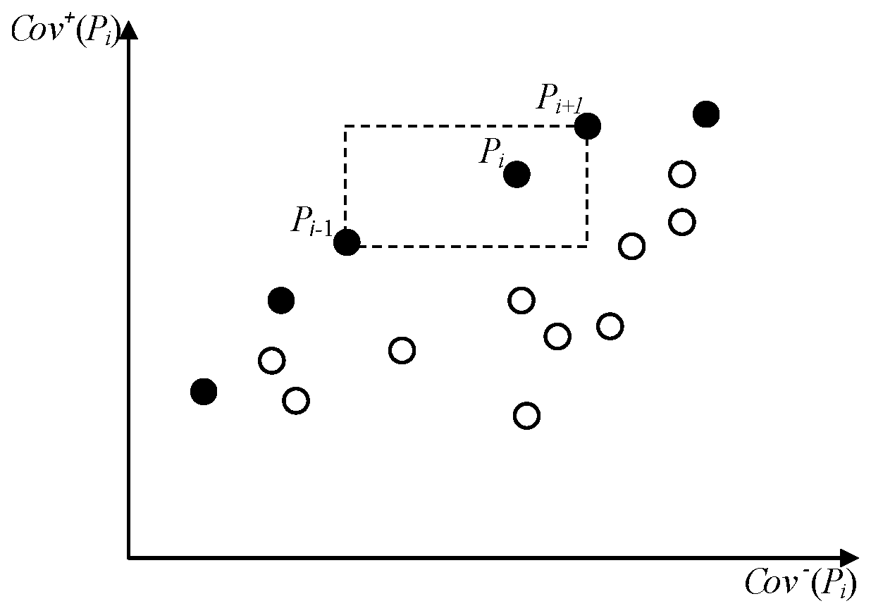
To estimate the density of solutions concerning the chosen solution, along each direction in the criteria space, two nearest solutions are found on both sides of the chosen solution. The distance between them is determined as the difference between the values of a different criterion. An estimate of the density of solutions near the selected point will be the average of the calculated distances, called the crowding distance. From the geometric point of view, it is possible to estimate the density by calculating the perimeter of the hypercube formed by the nearest neighboring solutions as vertices.

Figure 1 shows a graphical interpretation of the above approach for the case of our two objective functions (4). Solutions denoted as $p_{i+1}$ and $i-1$, which are nearest to the ith solutions and belong to the first front (filled dots), represent the vertices of the outlined rectangle (dotted line). Crowding distance, in this case, can be defined as the average length of the edges of the rectangle.

Calculating the crowding distance requires sorting the individuals in the population according to each objective function in ascending order of the value of this objective function. For individuals with the boundary value of the objective function (maximum or minimum), the crowding distance is assigned equal to infinity. All other intermediate solutions are assigned a distance value equal to the absolute value of the difference between the values of the functions of two neighboring solutions. This calculation continues for all objective functions. The final value of the crowding distance is calculated as the average of the individual values of the distances corresponding to each objective function. Pre-normalization of objective functions is recommended.

After all individuals in the population have been assigned to an estimate of the crowding distance, we can compare the solutions in terms of their degree of closeness to other solutions. A smaller value for the crowding distance indicates a higher density of solutions relative to the selected point. The density estimate is used in the crowded-comparison operator described below.

Crowded-Comparison Operator (${\prec }_n$) directs the evolutionary process of population transformation towards a fairly uniform distribution along the Pareto front.

We assume that each individual in the population has two attributes:

• Rank of dominance (front rank) $i_{rank}$;
• Crowding distance $i_{distance}$.

Then, the partial ordering is defined as follows. Individual i is preferred over individual j if the following conditions are met:

$$i{\prec }_{n}j⟺\left(i_{rank}<j_{rank}\right)\bigvee \left(i_{rank}=j_{rank}\bigwedge i_{distance}>j_{distance}\right).$$

(5)

Such ordering means that we prefer a solution with a lower (close to the first, which means the optimal front) rank between two solutions with different ranks. Otherwise, if both solutions are located in the same front, we prefer a solution located in areas where solutions are less crowded.

2.4.3. Basic Procedure of the NSGA-II

In this case, solving linear optimization problem is rather simple. Initially, the parent population $P_0$ is randomly created and sorted based on the dominance principle. Thus, the greater the suitability of an individual, the lower the value of its rank. Then, traditional genetic operators are applied: binary tournament selection, crossover, mutation, creating a child population $Q_0$ of a specified size N. Since elitism is introduced by comparing the current child population with the parent population, the procedure differs for the first generation from the repeated one.

Let the tth iteration of the algorithm be executed, at which the parent population $P_t$ generated the child population $Q_t$. A joint population $R_t=P_t\cup Q_t$ is then sorted according to the dominance principle. Thus, decisions that belong to the first front ${\mathcal{F}}_1$ and are not dominated should have a better chance of moving to the next generation population, which is ensured by the implementation of the elitism principle. If the first front ${\mathcal{F}}_1$ includes less than N members, then all members of this front move to the next population $P_{t+1}$. The remaining members of the population $P_{t+1}$ are selected from subsequent fronts in the order of their ranking. That is, the front ${\mathcal{F}}_2$ is included in the new parent population $P_{t+1}$, then the front ${\mathcal{F}}_3$, and so on. This procedure continues until the inclusion of the next front leads to an excess of the population size N. Let the front ${\mathcal{F}}_l$ no longer be included in the new population as a whole. To select members of the front ${\mathcal{F}}_l$ who will be included in the next generation, we sort the solutions of this front using the crowded-comparison operator and select the best solutions to supplement the population $P_{t+1}$. Now, a new population $P_{t+1}$ of size N can be used to apply selection, crossover, and mutation operators. It is important to note that the tournament selection binary operator is still used, but now, it is based on the crowded-comparison operator ${\prec }_n$, to use which, in addition to determining the rank, it is necessary to calculate the crowding distance for each member of the population $P_{t+1}$.

The schematic procedure of the NSGA-II algorithm originally proposed in [55] is shown in Figure 2.

Thus, a successful distribution of solutions within one front is realized by using the crowded-comparison procedure, which is also used in the individuals selection. Since the solutions compete with their crowding distances (a measure of the solution’s density in a neighborhood), the algorithm does not require any additional parameter determining the size of niches in the search space. The proposed crowding distance is calculated in the function space, but it can be implemented in the parameter space if necessary.

2.5. Our Approach: An Evolutionary Algorithm for Pattern Generation

The pattern $P_a$ is determined by baseline observation $a=\left\{x_1,x_2,\dots ,x_p\right\}$ and values of control variables $Y=\left\{y_1^{\left(a\right)},\dots ,y_p^{\left(a\right)}\right\}$ that are binary values. Thus, the solution to the problem of pattern generation is a set of points in the space of control variables that approximate the Pareto front for a given base observation.

The posed problem of finding logical patterns determines the binary representation of solutions in the form of binary strings, rather than real variables, as was postulated in the original NSGA-II. The binary representation of the solution also determined the list of available crossover and mutation operators, among which uniform crossover and mutation by gene inversion were chosen [63,64].

In addition, the crowding distance in space “the number of covered observations of the base class” requires a different interpretation—“the number of covered observations of the class other than the base”. Firstly, uniform coverage of the Pareto front is not required, since a preferable area is an area with a smaller scope of observations of the opposite class. Figure 3 illustrates this position: points of one Pareto front are colored according to their preference, with white color meaning less preference.

Taking into account these preconditions, the crowding distance was replaced by one of the heuristic definitions of informativity [3]:

$$I=\sqrt{Co{v}^{+}\left(P_a\right)}-\sqrt{Co{v}^{-}\left(P_a\right)}.$$

(6)

Similar to the crowding distance, the more preferable the individual, the greater the informative value.

Special attention is paid to the formation of the initial set of individuals. The usual approach is a uniform discrete distribution for values 0 and 1. However, based on the nature of the problem, an equal probability of dropping out 0 and 1 will mean, on average, the fixation of half of the features in the initial population, which gives rise to overly selective patterns. Therefore, the discrete distribution of values in the original population is defined differently: dropout 1 with probability p, and dropout 0 with probability $1-p$. The value p will be the hyperparameter of the genetic algorithm.

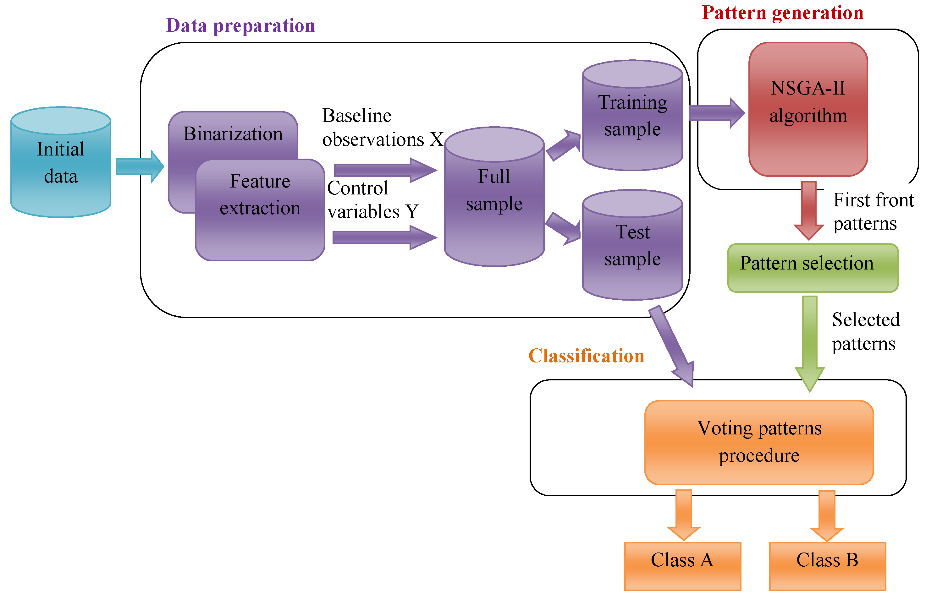
Figure 4 shows a diagram of the developed approach to construct a classifier using the NSGA-II algorithm for pattern generation. The NSGA-II algorithm is run independently for each baseline observation. The launch result is a set of patterns of the first front. The sets of patterns obtained for each baseline observation were combined into one complete set of patterns, which can be reduced using the selection procedure [2,65]. When recognizing control (or new) observations, the decision about the class is made by balanced voting of patterns on the observation under consideration [8].

A detailed description of pattern generation procedure from Figure 4 is presented in a form of pseudocode (Algorithms 1 and 2).

Algorithm 1 Fast-non-dominated-sorting

Require:  Evaluated population $P=\left\{P_1,\cdots ,P_N\right\}$, number of solutions in population N. 1: for each $P_i$, $i\in \left\{\overline{1,N}\right\}$ do 2:  for each $P_j$, $j\in \left\{\overline{1,N}\right\}$ do 3:   if $P_i$ dominates $P_j$ ($P_i\prec P_j$) then 4:    increase the set of solutions which the current solution dominates: $S_{P}i\leftarrow S_{P}i\cup \left\{P_j\right\}$ 5:   else 6:    if $P_j$ dominates $P_i$ ($P_j\prec P_i$) then 7:     increase the number of solutions which dominate the current solution: $n_{P}i\leftarrow n_{P}i+1$ 8:    end if 9:   end if 10:  end for 11:  if no solution dominates $P_i$, $(n_{P}i=0)$ then 12:   $P_i$ is a member of the first front: ${\mathcal{F}}_1\leftarrow {\mathcal{F}}_1\cup \left\{P_i\right\}$ 13:  end if 14: end for 15: $t\leftarrow 1$ 16: while${\mathcal{F}}_t\ne \varnothing$do 17:  $\mathcal{H}\leftarrow \varnothing$ 18:  for each $P_i\in {\mathcal{F}}_t$ do 19:   for each $P_j\in S_{P}i$ do 20:    $n_{P}j\leftarrow n_{P}j-1$ 21:    if $n_{P}j=0$ then 22:     $\mathcal{H}\leftarrow \mathcal{H}\cup \left\{P_j\right\}$ 23:    end if 24:   end for 25:  end for 26:  $t\leftarrow t+1$ 27:  ${\mathcal{F}}_t\leftarrow \mathcal{H}$ 28: end while 29: return a list of the non-dominated fronts $\mathcal{F}$

NSGA-II is one of the popular multiobjective optimization algorithms. It is usually assumed that each individual in the population represents a separate solution to the problem. Thus, the population is a set of non-dominated solutions, from which one or more solutions can then be selected, depending on which criteria are given the highest priority. A distinctive feature of the proposed algorithm is, among other things, that the solution to the problem is the entire population, in which individual members represent individual patterns.

Algorithm 2 An evolutionary algorithm for pattern generation

Require:  The set of baseline observations X and values of control variables Y 1: Create a random parent population $P_0$ of size N from X and Y 2: $\mathcal{F}\leftarrow Fast-nondominated-sort\left(P_0\right)$ 3: Create a child population of size N using selection, crossover and mutation procedures $Q_0\leftarrow Child\left(P_0\right)$ 4: $t\leftarrow 0$ 5: while termination criteria not met do 6:  Combine parent and child populations $R_t\leftarrow P_t\cup Q_t$. The size of population $R_t$ is $2N$ 7:  $\mathcal{F}\leftarrow Fast-nondominated-sort\left(R_t\right)$ 8:  while $|P_{t+1}|\ge N$ do 9:   $I\leftarrow \sqrt{Co{v}^{+}\left(P_{t+1}\right)}-\sqrt{Co{v}^{-}\left(P_{t+1}\right)}$ 10:    $P_{t+1}\leftarrow P_{t+1}\cup {\mathcal{F}}_i$ 11:   end while 12:   Sort $P_{t+1}$ in descending order 13:   $P_{t+1}\leftarrow thefirstNelementsfrom{P}_{t+1}$ 14:   Create a child population using selection, crossover and mutation procedures $Q_{t+1}\leftarrow Child\left(P_{t+1}\right)$ 15:   $t\leftarrow t+1$ 16: end whilereturn$P_{t+1}$

3. Application of the Proposed Method to Problems in Healthcare

The proposed approach relates to interpretable machine learning methods. Therefore, experimental studies were carried out on problems in which the interpretability of the recognition model and the possibility of a clear explanation of the solution proposed by the classifier are of great importance. The results are shown on two datasets: breast cancer diagnosis (the dataset from the UCI repository [66]) and predicting complications of myocardial infarction (regional data [67]).

3.1. Breast Cancer Diagnosis

The problem of diagnosing breast cancer on a sample collected in Wisconsin is considered (Breast Cancer Wisconsin, BCW) [66]. Since the attributes in the data take on numeric (integer) values, their binarization is necessary, that is, the transition to new binary features. Threshold-based binarization is used. Based on the original value x, a new binary variable $x_t$ can be constructed as follows:

$$x_t=\left\{\begin{array}{cc}1,& \mathrm{if}x\ge t,\\ 0,& \mathrm{if}x<t,\end{array}\right.$$

(7)

where t is a cut point (threshold value).

As a result of executing the binarization procedure, 72 binary attributes were obtained from 9 initial attributes. The original dataset is divided in the ratio of 70% and 30% into training and test samples (in a random way), which results in 478 and 205 observations, respectively. To search for logical patterns, objects of the training sample (both positive and negative classes) consistently act as a baseline observation. For each baseline observation, the NSGA-II algorithm is run independently with the following parameters:

• Parent population size: 20;
• Descendant population size: 20;
• Number of generations: 10;
• Probability of mutation (for each decision variable): 5%;
• Cross type: uniform.

The final set of patterns includes patterns of the first front from the last population of solutions. The first front can contain one or several patterns. Thus, the final set of patterns is completed based on covering the observations of the training sample. Therefore, each observation will be covered by at least one pattern from this set.

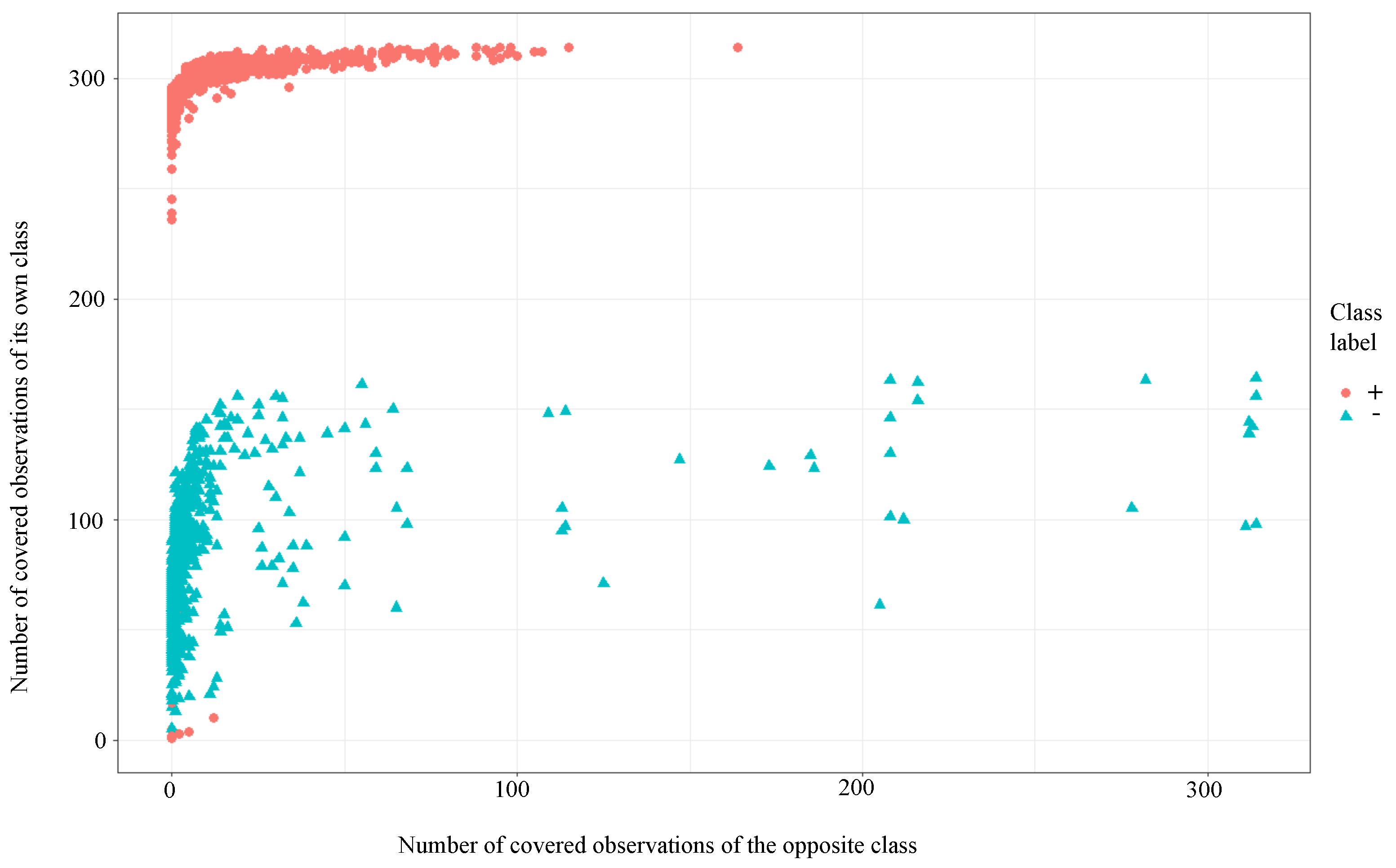
A series of experiments are carried out with a different probability of dropping one when initializing control variables in the first population of the genetic algorithm. The following probabilities were used: $p\in \{0.5,0.3,0.1\}$. A complete set of patterns was independently constructed for each probability. This set included the patterns of the first fronts obtained using the NSGA-II algorithm with the sequential acceptance of the observations of the training sample as a baseline observation. The resulting complete set of patterns are shown in Figure 5 in the coordinates of the number of covered observations of its own and the opposite class.

Figure 6 shows the resulting full set of patterns for the value $p=0.3$.

Figure 7 shows the resulting full set of patterns for the value $p=0.1$.

Table 1. Distribution of patterns in terms of power.

	Probability of Dropping 1 on Initialization
The Number of Covered Observations of The Same Class on The Training Sample	p = 0.5	p = 0.3	p = 0.1
1	1240	200	20
from 1 to 5	394	113	4
from 5 to 100	106	268	545
from 100 to 300	465	974	1770
above 300	0	3	962
Total number of patterns detected	2205	1558	3301

shows the distribution of patterns by power. Power is understood as the number of covered observations of its class included in the training sample. Data on the aggregate set of patterns are given without considering their class affiliation.

In the case of equally probable dropping of zero and one during initialization, a large number of trivial patterns are found, that is, patterns that cover only the basic observation and do not cover any more observations. These patterns are overly selective. With a decrease in the probability of dropping one during initialization, the selectivity of the obtained patterns decreases, thereby increasing their coverage. However, increased coverage affects the accuracy of initiated patterns, i.e., the number of observations from the opposite class.

The results of the classification of test observations compared to actual values are shown in

Table 2. Confusion matrix for BCW problem.

p = 0.5			p = 0.3			p = 0.1
	Original Class			Original Class			Original Class
Classifier Prediction	−	+	Classifier Prediction	−	+	Classifier Prediction	−	+
−	126	4	−	128	8	−	128	12
+	0	37	+	2	65	+	2	63
?	4	34	?	0	2	?	−	−
Accuracy	0.888		Accuracy	0.946		Accuracy	0.932

. Symbols “+” and “−” denote the class labels introduced above. The symbol “?” means the impossibility of classification because none of the patterns is valid for observation.

Thus, a significant influence of the probability of dropping one is established during the initialization of control variables in the first population of the multi-criteria genetic algorithm. This parameter affects the selectivity of the detected patterns. The equiprobable dropping of zero and one entails a significant proportion of baseline observations, for which only patterns that cover only the baseline observation and no other training observations are found.

3.2. Predicting the Complication of Myocardial Infarction

The problem of predicting the development of complications of myocardial infarction is considered [67]. Datasets are often significantly asymmetric: one of the classes significantly outnumbers the other in terms of the number of objects. In our case, a sample contains data on 1700 cases with an uneven division into classes: 170 cases with complications, and 1530 cases without. Each case in the initial sample is described by 127 attributes containing information about the history of each patient, the clinical picture of the myocardial infarction, electrographic and laboratory parameters, drug therapy, and the characteristics of the course of the disease in the first days of myocardial infarction. Data include the following types: textual data, integer values, rank scale values with known range, real and binary values. A more detailed description of the attributes is given in

Table 3. Description of sample attributes for myocardial infarction problem.

Attribute Number	Description	Value Type
1	Full name of the patient (meta attribute)	text
2	Age	integer
3	Gender	binary
4–34	The presence or absence of various pathologies in the cardiovascular, endocrine and respiratory systems before the development of myocardial infarction	rank, binary
35–38	Blood pressure according to the data of the cardiology team and the admission department	integer
39–44	Complications arising at the time of transportation of the patient to the clinic or at the time of hospitalization	binary
45–49	Depth and localization of cardiac muscle necrosis	rank, binary
50–75	ECG characteristics at the time of admission of the patient to the intensive care unit	binary
76–82	The use of drugs during fibrinolytic therapy	binary
83–86	Electrolyte shifts in the blood	binary, real
87–92	Laboratory characteristics of blood	real, rank
93–115	The course of the disease in the first days of myocardial infarction	rank, binary
116–127	The occurrence of complications of myocardial infarction or the outcome of this disease	rank, binary

.

The problem of predicting atrial fibrillation (AF) is solved, assuming that it is described by the variable 116 (target variable, 1—the occurrence of atrial fibrillation, 0—its absence). According to the nature of the attributes, variables $94,95,97,98,104,105,107,108$ were excluded since these values could be obtained after the occurrence of complications [67]. The exclusion of these attributes significantly complicates the forecasting task. Thus, the number of predictors from the initial data was 107 variables.

The properties of the data used are as follows:

• A significant number of missing values;
• “Asymmetry” of the sample: the number of patients with atrial fibrillation is only about 10% of the total;
• The presence of different types of attributes;
• The use of homogeneous patterns leads to overfitting (the formation of patterns with a large number of conditions and a very small coverage).

Two approaches to data processing were implemented when constructing the classifier, as described below.

3.2.1. First Approach to Data Preparation (Complete Data and Handling of Missing Values)

The data contained a significant number of missing values. Columns with more than 100 missing values were excluded (47 variables). The remaining variables contained rank scale values and binary values. Missing values in columns containing 100 or less gaps were filled with the mode value. Thus, the prepared dataset contained 60 variables (not including the target).

The binarization for the values presented on the rank scale was performed based on the following rules. Based on the original variable x, a new binary variable $x_t$ was constructed as follows:

$$x_t=\left\{\begin{array}{cc}1,& \mathrm{if}x=r,\\ 0,& \mathrm{if}x\ne r,\end{array}\right.$$

(8)

where r is the value of the original variable $x,r\in R$, such that R is a known set of all possible values of a variable x. As a result of the binarization procedure, the total number of binary variables was 119.

The original dataset is divided in a ratio of 70% and 30% into training and test samples, that is 1190 and 510 observations, respectively. To search for patterns, the training sample’s objects (both positive and negative classes) consistently act as a baseline observation. For each baseline observation, the NSGA-II algorithm is run independently with the following parameters:

• Parent population size: 20;
• Descendant population size: 20;
• Number of generations: 10;
• Probability of dropping one on initialization: 0.05;
• Probability of mutation (for each decision variable): 0.5%;
• Crossing type: uniform.

More resources are allocated for seeking positive class observations. The sizes of the parent and descendant populations are 50, and the number of generations was 100. As a result, a complete set of patterns was obtained, containing 1961 positive class patterns and 6148 negative class patterns. A classifier is built that decides on a new observation by a simple voting. The results of the classification of the test observations compared to the actual values are shown in

Table 4. Confusion matrix for AF problem (first approach).

	Original Class
Classifier Prediction	−	+
−	347	31
+	109	23
Accuracy	0.7255

. Symbols “+" and “−” denote the class labels introduced above.

Thus, the classifier arising from data for which missing values were processed did not show an acceptable result of classifying positive class objects, which may be caused by deleting essential data due to missing values processing. Since logical patterns are usable for classifying data with missing values, a different approach to data preparation was used, which is described below.

3.2.2. Another Approach to Data Preparation (Reduced Sampling without Processing Missing Values)

The second approach to data preparation is to store the missing attribute values as in the original sample. The class imbalance problem is also solved by randomly selecting a subset of objects of the prevailing class, equal in cardinality to the set of objects of another class.

As a result, the original sample was reduced to 338 cases, with an equal number of instances belonging to each class. Observations are described by 106 variables (not including the target). On the reduced sample, 8 variables take either just the same value, or the same value and gaps, so these variables were excluded from consideration. Among the remaining variables, 16 are rank variables, 12 are real, and the other variables are binary. Rank variables are transformed into several new binary variables, whose number is determined by the number of allowed ranks. Based on each real variable, four new binary variables are built. The threshold values of these variables were divided by the range of values of the original variables into four equal parts. As a result of applying the binarization procedure, the total number of variables was 200 (excluding the target variable).

Data were divided into training and test samples in the ratio of 80% and 20%, respectively, which causes 270 and 68 observations, respectively, in the same number of observations of positive and negative classes. For each training set observation, the NSGA-II algorithm is run independently with the following parameters:

• Parent population size: 20;
• Descendant population size: 20;
• Number of generations: 10;
• Probability of dropping one on initialization: 0.05;
• Probability of mutation (for each decision variable): 0.5%;
• Crossing type: uniform.

As a result, the cumulative set of patterns for the first front includes 2259 rules for the positive class and 2403 for the negative class. The classifiers are built based on reduced sets with the selection according to informativeness (I) of revealed patterns. Simple voting of patterns classifies a new observation. If the attribute value fixed in the pattern is unknown in the new observation, we assume that this pattern does not cover this observation. The classification results for different threshold values of informativeness are shown in

Table 5. Confusion matrix for AF problem (the second approach).

I > 0			I > 1			I > 2
	Original Class			Original Class			Original Class
Classifier Prediction	−	+	Classifier Prediction	−	+	Classifier Prediction	−	+
−	25	7	−	25	7	−	25	5
+	9	27	+	9	27	+	9	29
Accuracy	0.7647		Accuracy	0.7647		Accuracy	0.7941
I> 0			I> 1			I> 2
	Original Class			Original Class			Original Class
Classifier Prediction	−	+	Classifier Prediction	−	+	Classifier Prediction	−	+
−	23	4	−	23	3	−	30	18
+	11	30	+	11	31	+	4	16
Accuracy	0.7794		Accuracy	0.7941		Accuracy	0.6765

.

Thus, the greatest accuracy is achieved when selecting patterns with informativeness greater than 2 or greater than 4. Since the importance of correctly identifying positive class objects (true positive rate or sensitivity) is greater than a negative one (true negative rate or specificity), the best option is to select patterns with informativeness greater than 4, since the accuracy of classifying objects in the positive class is higher. The obtained classification accuracy exceeds the accuracy obtained in [44].

Let us explore some characteristics of the resulting patterns when choosing patterns based on $I\ge 4$.

Table 6. Degree of the patterns.

	Amount	Min	1st Quartile	Median	Mean	3rd Quartile	Max
Positive patterns	96	3	6	7	7.802	9	16
Negative patterns	103	6	9	11	11.480	14	19
All patterns	199	3	7	9	9.704	12	19

shows the number of patterns as well as the degree distribution of these patterns, that is, the number of binary variables fixed in the pattern.

Figure 8 shows the indicated sets of patterns in the coordinates of the number of covered observations of its class and the opposite class. Figure 8 is given for the training sample.

Figure 9 shows the indicated sets of patterns in the coordinates of the number of covered observations of its class and the opposite class for the test sample.

To evaluate the efficiency of the proposed approach, we made a comparative study with some widely used machine learning classification algorithms. We compared the proposed multi-criteria genetic algorithm (MGA-LAD) with Support Vector Machine (SVM), C4.5 Decision Trees (J48), Random Forest (RF), Multilayer Perceptron (MP), and Simple Logistic Regression (LR) methods. The tests were performed on the following datasets from UCI Machine Learning Repository [66]: Wisconsin breast cancer (BCW), Hepatitis (Hepatitis), Pima Indian diabetes (Pima), Congressional voting (Voting). Results using 10-fold cross-validation are presented in

Table 7. Classification accuracy of the compared algorithms.

Dataset	ML	LAD, Fuzziness at Most $\mathsf{\phi }$					MGA-LAD
		$\mathsf{\phi }$=0	$\mathsf{\phi }$= 0.05	$\mathsf{\phi }$= 0.1	$\mathsf{\phi }$= 0.15	$\mathsf{\phi }$= 0.2
BCW	0.967 ± 0.01 (RF)	0.951 ± 0.03	0.953 ± 0.02	0.957 ± 0.03	0.966 ± 0.03	0.966 ± 0.03	0.965 ± 0.02
Hepatitis	0.858 ± 0.08 (SVM)	0.819 ± 0.09	0.826 ± 0.09	0.819 ± 0.09	0.806 ± 0.09	0.806 ± 0.08	0.847 ± 0.10
Pima	0.736 ± 0.03 (RF)	0.682 ± 0.02	0.687 ± 0.02	0.691 ± 0.02	0.687 ± 0.02	0.682 ± 0.02	0.749 ± 0.04
Voting	0.961 ± 0.01 (LR)	0.945 ± 0.03	0.952 ± 0.03	0.954 ± 0.03	0.954 ± 0.03	0.949 ± 0.03	0.973 ± 0.03

. Here, the “ML” column contains results for algorithms that give the highest accuracy among the commonly used machine learning algorithms. The best algorithm is given in parentheses. Another approach that has been used for comparison is logical analysis of data (LAD-WEKA in the WEKA package [68]) at various fixed fuzziness values φ (an upper bound on the number of points from another class that is covered by a pattern as a percentage of the total number of points covered by the pattern).

The value of the fuzziness parameter $\mathsf{\phi }$ affects the size, coverage, and informativeness of the resulting patterns and ultimately affects the classification accuracy. In LAD, it is necessary to find many a-pattern based on different baseline observations. However, for each such pattern, the most appropriate fuzziness value may be different. Using a two-criteria model and the corresponding optimization algorithm allows us to find a set of Pareto optimal patterns without the need to fix the fuzziness value, which expands the possibilities of LAD and can improve the classification accuracy.

4. Discussion

In the previous section, we described the application of the proposed approach to solving practical medical classification problems.

The first dataset describes tissue characteristics to diagnose benign or malignant breast neoplasm. This dataset was studied many times before, for example [69,70], including the approach based on LAD [2]. For this example, we established a significant influence of the introduced hyperparameter of the genetic algorithm—the probability of dropping one during the initialization of the initial population, which is the fixation of the attribute’s value in the pattern according to its value in the baseline observation. High values of this probability lead to low classification accuracy due to excessive selectivity of patterns and, accordingly, an increase in the number of objects with a refusal to determine the class membership.

The second dataset is the problem of predicting complications of myocardial infarction-atrial fibrillation. In this case, two approaches are implemented to handle missing values in the data. The first, typical for most data mining algorithms, is a combination of deleting values with missing values and filling them in. In this case, satisfactory classification results were not achieved when a complete dataset with a significantly larger presence of objects of one of the classes was used. In the second approach, the missing values are not preprocessed since the set of logical patterns as a whole has no restrictions in classifying observations with missing values. In addition, we use a reduced sample with an equal number of observations for each of the classes.

Homogeneous patterns in this dataset have small coverage, and using only homogeneous patterns leads to overfitting. Relaxation of homogeneity constraints requires adjusting the threshold (right-hand side of the constraint), which can be difficult since, when solving pattern finding problems, the best balance between coverage and homogeneity for a single pattern can be far from the best for another pattern (based on another baseline observation). The proposed approach simplifies the search for this balance since it considers many Pareto-optimal patterns. This approach prevents overfitting in contrast with using only homogeneous patterns or patterns with a given threshold for homogeneity. At the same time, the accuracy reaches the values obtained using an artificial neural network specially developed for these data [67]. The classification results are also comparable with the results of other works on this topic [71,72].

5. Conclusions

Logical analysis of data is a two-class learning method dealing with features that can be binarized. Logical analysis of data consists of several stages, and the formation of patterns is the most important. Finding pure patterns is a single-criteria optimization problem that consists of finding a pattern that covers as many positive observations as possible and does not cover negative observations. With a more general formulation, which allows making mistakes for a pattern, the problem turns into a search for a compromise between the completeness of the range of observations of some target class and the minimization of the coverage of observations that do not belong to the target class.

In this study, we used an approach to find patterns in the form of an approximation of the Pareto-optimal front and proposed evolutionary algorithms for solving such a problem due to their potential ability to cover the front. We modified the NSGA-II for pattern searching and tested it on several application problems from the repository.

Results of our work enabled us to find more informative patterns in the data, taking into account the coverage of objects of different classes. We compared our modified algorithm with commonly used machine learning algorithms on four classification problems. The results were comparable, and in some cases better than results of classical ML algorithms which do not meet the requirement of the interpretability of the result.

Our experiments discovered a significant influence of the probability of dropping one of the control variables of the initial population in the multi-criteria genetic algorithm. This parameter affects the selectivity of the selected patterns. So, the equal probability of zero and one entails a significant proportion of baseline observations, for which only patterns are found that cover only the baseline observation and no other observation of the training sample.

Since our two-criteria optimization model in a combination with the developed modification of the genetic algorithm does not require the number or ratio of observations of the opposite class to be pre-set. Thus, our approach is a more versatile tool of data analysis in this sense than known methods for the fuzzy patterns generation. The method considered in this paper could be useful for the classification tasks in, for instance, healthcare system, faults diagnosis and any problems in which the interpretability of results are of great importance.