An Accelerated Fixed-Point Algorithm with an Inertial Technique for a Countable Family of G-Nonexpansive Mappings Applied to Image Recovery

Abstract

Many authors have proposed fixed-point algorithms for obtaining a fixed point of G-nonexpansive mappings without using inertial techniques. To improve convergence behavior, some accelerated fixed-point methods have been introduced. The main aim of this paper is to use a coordinate affine structure to create an accelerated fixed-point algorithm with an inertial technique for a countable family of G-nonexpansive mappings in a Hilbert space with a symmetric directed graph G and prove the weak convergence theorem of the proposed algorithm. As an application, we apply our proposed algorithm to solve image restoration and convex minimization problems. The numerical experiments show that our algorithm is more efficient than FBA, FISTA, Ishikawa iteration, S-iteration, Noor iteration and SP-iteration.

1. Introduction

Let H be a real Hilbert space with the norm $\parallel ·\parallel$ and C be a nonempty closed convex subset of $H.$ A mapping $T:C\to C$ is said to be nonexpansive if it satisfies the following symmetric contractive-type condition:

$$\parallel Tx-Ty\parallel \le \parallel x-y\parallel ,$$

for all $x,y\in C$; see [1].

The notation of the set of all fixed points of T is $F\left(T\right):=\{x\in C:x=Tx\}.$

Many mathematicians have studied iterative schemes for finding the approximate fixed-point theorem of nonexpansive mappings over many years; see [2,3]. One of these is the Picard iteration process, which is well known and popular. Picard’s iteration process is defined by

$$x_{n+1}=T{x}_n,$$

where $n\ge 1$ and an initial point $x_1$ is randomly selected.

The iterative process of Picard has been developed extensively by many mathematicians, as follows:

Mann iteration process [4] is defined by

$$\begin{array}{c}\hfill x_{n+1}=(1-{\rho }_n)x_n+{\rho }_{n}T{x}_n,\end{array}$$

(1)

where $n\ge 1$ and an initial point $x_1$ is randomly selected and $\left\{{\rho }_n\right\}$ is a sequence in $[0,1]$.

Ishikawa iteration process [5] is defined by

$$\begin{array}{c}\hfill \left\{\begin{array}{c}{y}_n=(1-{\zeta }_n)x_n+{\zeta }_{n}T{x}_n,\hfill \\ x_{n+1}=(1-{\rho }_n)x_n+{\rho }_{n}T{y}_n,\hfill \end{array}\right.\end{array}$$

(2)

where $n\ge 1$ and an initial point $x_1$ is randomly selected and $\left\{{\zeta }_n\right\}$, $\left\{{\rho }_n\right\}$ are sequences in $[0,1]$.

S-iteration process [6] is defined by

$$\begin{array}{c}\hfill \left\{\begin{array}{c}{y}_n=(1-{\zeta }_n)x_n+{\zeta }_{n}T{x}_n,\hfill \\ x_{n+1}=(1-{\rho }_n)T{x}_n+{\rho }_{n}T{y}_n,\hfill \end{array}\right.\end{array}$$

(3)

where $n\ge 1$ and an initial point $x_1$ is randomly selected and $\left\{{\zeta }_n\right\}$, $\left\{{\rho }_n\right\}$ are sequences in $[0,1]$. We know that the S-iteration process (3) is independent of Mann and Ishikawa iterative schemes and converges quicker than both; see [6].

Noor iteration process [7] is defined by

$$\begin{array}{c}\hfill \left\{\begin{array}{c}{z}_n=(1-{\eta }_n)x_n+{\eta }_{n}T{x}_n,\hfill \\ y_n=(1-{\zeta }_n)x_n+{\zeta }_{n}T{z}_n,\hfill \\ x_{n+1}=(1-{\rho }_n)x_n+{\rho }_{n}T{y}_n,\hfill \end{array}\right.\end{array}$$

(4)

where $n\ge 1$ and an initial point $x_1$ is randomly selected and $\left\{{\eta }_n\right\},$$\left\{{\zeta }_n\right\}$, $\left\{{\rho }_n\right\}$ are sequences in $[0,1]$. We can see that Mann and Ishikawa iterations are special cases of the Noor iteration.

SP-iteration process [8] is defined by

$$\begin{array}{c}\hfill \left\{\begin{array}{c}{z}_n=(1-{\eta }_n)x_n+{\eta }_{n}T{x}_n,\hfill \\ y_n=(1-{\zeta }_n)z_n+{\zeta }_{n}T{z}_n,\hfill \\ x_{n+1}=(1-{\rho }_n)y_n+{\rho }_{n}T{y}_n,\hfill \end{array}\right.\end{array}$$

(5)

where $n\ge 1$ and an initial point $x_1$ is randomly selected and $\left\{{\eta }_n\right\},$$\left\{{\zeta }_n\right\}$, $\left\{{\rho }_n\right\}$ are sequences in $[0,1]$. We know that Mann, Ishikawa, Noor and SP-iterations are equivalent and the SP-iteration converges faster than the other; see [8].

The fixed-point theory is a rapidly growing field of research because of its many applications. It has been found that a self-map on a set admits a fixed point under specific conditions. One of the recent generalizations is due to Jachymiski.

Jachymski [9] proved some generalizations of the Banach contraction principle in a complete metric space endowed with a directed graph using a combination of fixed-point theory and graph theory. In Banach spaces with a graph, Aleomraninejad et al. [10] proposed an iterative scheme for G-contraction and G-nonexpansive mappings. G-monotone nonexpansive multivalued mappings on hyperbolic metric spaces endowed with graphs were defined by Alfuraidan and Khamsi [11]. On a Banach space with a directed graph, Alfuraidan [12] showed the existence of fixed points of monotone nonexpansive mappings. For G-nonexpansive mappings in Hilbert spaces with a graph, Tiammee et al. [13] demonstrated Browder’s convergence theorem and a strong convergence theorem of the Halpern iterative scheme. The convergence theorem of the three-step iteration approach for solving general variational inequality problems was investigated by Noor [7]. According to [14,15,16,17], the three-step iterative method gives better numerical results than the one-step and two-step approximate iterative methods. For approximating common fixed points of a finite family of G-nonexpansive mappings, Suantai et al. [18] combined the shrinking projection with the parallel monotone hybrid method. Additionally, they used a graph to derive a strong convergence theorem in Hilbert spaces under certain conditions and applied it to signal recovery. There is also research related to the application of some fixed-point theorem on the directed graph representations of some chemical compounds; see [19,20].

Several fixed-point algorithms have been introduced by many authors [7,9,10,11,12,13,14,15,16,17,18] for finding a fixed point of G-nonexpansive mappings with no inertial technique. Among these algorithms, we need those algorithms that are efficient for solving the problem. So, some accelerated fixed-point algorithms have been introduced to improve convergence behavior; see [21,22,23,24,25,26,27,28]. Inspired by these works mentioned above, we employed a coordinate affine structure to define an accelerated fixed-point algorithm with an inertial technique for a countable family of G-nonexpansive mappings applied to image restoration and convex minimization problems.

This paper is divided into four sections. The first section is the introduction. In Section 2, we recall the basic concepts of mathematics, definitions, and lemmas that will be used to prove the main results. In Section 3, we prove a weak convergence theorem of an iterative scheme with the inertial step for finding a common fixed point of a countable family of G-nonexpansive mappings. Furthermore, we apply our proposed method for solving image restoration and convex minimization problems; see Section 4.

2. Preliminaries

The basic concepts of mathematics, definitions, and lemmas discussed in this section are all important and useful in proving our main results.

Let X be a real normed space and C be a nonempty subset of X. Let $▵=\left\{\right(u,u):u\in C\}$, where Δ stands for the diagonal of the Cartesian product $C\times C$. Consider a directed graph G in which the set $V\left(G\right)$ of its vertices corresponds to C, and the set $E\left(G\right)$ of its edges contains all loops, that is $E\left(G\right)\supseteq ▵.$ Assume that G does not have parallel edges. Then, $G=\left(V\right(G),E(G\left)\right)$. The conversion of a graph G is denoted by $G^{-1}$. Thus, we have

$$E\left(G^{-1}\right)=\{(u,v)\in C\times C:(v,u)\in E\left(G\right)\}.$$

A graph G is said to be symmetric if $(x,y)\in E\left(G\right)$; we have $(y,x)\in E\left(G\right)$.

A graph G is said to be transitive if for any $u,v,w\in V\left(G\right)$ such that $(u,v),$$(v,w)\in E(G,)$; then, $(u,w)\in E\left(G\right).$

Recall that a graph G is connected if there is a path between any two vertices of the graph $G.$ Readers might refer to [29] for additional information on some basic graph concepts.

We say that a mapping $T:C\to C$ is said to be G-contraction [9] if T is edge preserving, i.e., $(Tu,Tv)\in E\left(G\right)$ for all $(u,v)\in E\left(G\right)$, and there exists $\rho \in [0,1)$ such that

$$\parallel Tu-Tv\parallel \le \rho \parallel u-v\parallel$$

for all $(u,v)\in E\left(G\right),$ where $\rho$ is called a contraction factor. If T is edge preserving, and

$$\parallel Tu-Tv\parallel \le \parallel u-v\parallel$$

for all $(u,v)\in E\left(G\right)$, then T is said to be G-nonexpansive; see [13].

A mapping $T:C\to C$ is called G-demiclosed at 0 if for any sequence $\left\{u_n\right\}\subseteq C,$$(u_n,u_{n+1})\in E\left(G\right),$$u_n\rightharpoonup u$ and $T{u}_n\to 0$; then, $Tu=0$.

To prove our main result, we need to introduce the concept of the coordinate affine of the graph $G=\left(V\right(G),E(G\left)\right)$. For any $\alpha$, $\beta \in \mathbb{R}$ with $\alpha +\beta =1,$ we say that $E\left(G\right)$ is said to be left coordinate affine if

$$\alpha (x,y)+\beta (u,y)\in E\left(G\right)$$

for all $(x,y)$, $(u,y)\in E\left(G\right).$ Similar to this, $E\left(G\right)$ is said to be right coordinate affine if

$$\alpha (x,y)+\beta (x,z)\in E\left(G\right)$$

for all $(x,y)$, $(x,z)\in E\left(G\right).$

If $E\left(G\right)$ is both left and right coordinate affine, then $E\left(G\right)$ is said to be coordinate affine.

The following lemmas are the fundamental results for proving our main theorem; see also [21,30,31].

Lemma 1

([30]). Let $\left\{v_n\right\},\left\{w_n\right\}$ and $\left\{{\vartheta }_n\right\}\subset {\mathbb{R}}^{+}$ such that

$$v_{n+1}\le (1+{\vartheta }_n)v_n+w_n,$$

where $n\in \mathbb{N}.$ If ${\sum }_{n=1}^{\infty }{\vartheta }_n<\infty$ and ${\sum }_{n=1}^{\infty }{w}_n<\infty ,$ then ${lim}_{n\to \infty }{v}_n$ exists.

Lemma 2

([31]). For a real Hilbert space H, the following results hold:

(i) For any $u,v\in H$ and $\gamma \in [0,1],$

$${\parallel \gamma u+(1-\gamma )v\parallel }^2={\gamma \parallel u\parallel }^2+{(1-\gamma )\parallel v\parallel }^2-\gamma (1-\gamma ){\parallel u-v\parallel }^2.$$

(ii) For any $u,v\in H,$

$${\parallel u\pm v\parallel }^2={\parallel u\parallel }^2\pm 2⟨u,v⟩+{\parallel v\parallel }^2.$$

Lemma 3

([21]). Let $\left\{v_n\right\}$ and $\left\{{\mu }_n\right\}\subset {\mathbb{R}}^{+}$ such that

$$v_{n+1}\le (1+{\mu }_n)v_n+{\mu }_n{v}_{n-1},$$

where $n\in \mathbb{N}.$ Then,

$$v_{n+1}\le M·\prod _{j=1}^n(1+2{\mu }_j),$$

where $M=max\{v_1,v_2\}.$ Furthermore, if ${\sum }_{n=1}^{\infty }{\mu }_n<\infty ,$ then $\left\{v_n\right\}$ is bounded.

Let $\left\{u_n\right\}$ be a sequence in $X.$ We write $u_n\rightharpoonup u$ to indicate that a sequence $\left\{u_n\right\}$ converges weakly to a point $u\in H.$ Similarly, $u_n\to u$ will symbolize the strong convergence. For  $v\in C,$ if there is a subsequence $\left\{u_{n_k}\right\}$ of $\left\{u_n\right\}$ such that $u_{n_k}\rightharpoonup v,$ then v is called a weak cluster point of $\left\{u_n\right\}.$ Let ${\omega }_w\left(u_n\right)$ be the set of all weak cluster points of $\left\{u_n\right\}.$

The following lemma was proved by Moudafi and Al-Shemas; see [32].

Lemma 4

([32]). Let $\left\{u_n\right\}$ be a sequence in a real Hilbert space H such that there exists $\mathsf{\varnothing }\ne \mathsf{\Lambda }\subset H$ satisfying:

(i) For any $p\in \mathsf{\Lambda },{lim}_{n\to \infty }\parallel u_n-p\parallel$ exists.

(ii) Any weak cluster point of $\left\{u_n\right\}\in \mathsf{\Lambda }.$

Then, there exists $x^{*}\in \mathsf{\Lambda }$ such that $u_n\rightharpoonup x^{*}.$

Let $\left\{T_n\right\}$ and $\psi$ be families of nonexpansive mappings of C into itself such that $⌀\ne F\left(\psi \right)\subset {\cap }_{n=1}^{\infty }F\left(T_n\right),$ where $F\left(\psi \right)$ is the set of all common fixed points of each $T\in \psi .$ A sequence $\left\{T_n\right\}$ satisfies the NST-condition (I) with $\psi$ if, for any bounded sequence $\left\{u_n\right\}$ in $C,$

$$\underset{n\to \infty }{lim}\parallel T_n{u}_n-u_n\parallel =0\mathrm{implies}\underset{n\to \infty }{lim}\parallel T{u}_n-u_n\parallel =0,$$

for all $T\in \psi$; see [33]. If $\psi =\left\{T\right\},$ then $\left\{T_n\right\}$ satisfies the NST-condition (I) with $T.$

The forward–backward operator of lower semi-continuous and convex functions of $f,g:{\mathbb{R}}^n\to (-\infty ,+\infty ]$ has the following definition:

A forward-backward operator T is defined by $T:=pro{x}_{\lambda g}(I-\lambda \nabla f)$ for $\lambda >0$, where $\nabla f$ is the gradient operator of function f and $pro{x}_{\lambda g}x:=argmi{n}_{y\in H}\left\{g\left(y\right)+\frac{1}{2\lambda }{\parallel y-x\parallel }^2\right\}$ (see [34,35]). Moreau [36] defined the operator $pro{x}_{\lambda g}$ as the proximity operator with respect to $\lambda$ and function g. Whenever $\lambda \in (0,2/L)$, we know that T is a nonexpansive mapping and L is a Lipschitz constant of $\nabla f$. We have the following remark for the definition of the proximity operator; see [37].

Remark 1.

Let $g:{\mathbb{R}}^n\to \mathbb{R}$ be given by $g\left(x\right)={\lambda \parallel x\parallel }_1$. The proximity operator of g is evaluated by the following formula

$$pro{x}_{{\lambda \parallel ·\parallel }_1}\left(x\right)=(sign\left(x_i\right)max\left(\right|x_i{|-\lambda ,0))}_{i=1}^n,$$

where $x=(x_1,x_2,\cdots ,x_n)$ and ${\parallel x\parallel }_1={\sum }_{i=1}^n\left|x_i\right|$.

The following lemma was proved by Bassaban et al.; see [22].

Lemma 5.

Let H be a real Hilbert space and T be the forward–backward operator of f and g, where g is a proper lower semi-continuous convex function from H into $\mathbb{R}\cup \{\infty \}$, and f is a convex differentiable function from H into $\mathbb{R}$ with gradient $\nabla f$ being L-Lipschitz constant for some $L>0$. If $\left\{T_n\right\}$ is the forward–backward operator of f and g such that $a_n\to a$ with a, $a_n\in (0,2/L)$, then $\left\{T_n\right\}$ satisfies the $NST$-condition (I) with T.

3. Main Results

In this section, we obtain a useful proposition and a weak convergence theorem of our proposed algorithm by using the inertial technique.

Let C be a nonempty closed and convex subset of a real Hilbert space H with a directed graph $G=\left(V\right(G),E(G\left)\right)$ such that $V\left(G\right)=C$. Let $\left\{T_n\right\}$ be a family of G-nonexpansive mappings of C into itself such that $\varnothing \ne {\cap }_{n=1}^{\infty }F\left(T_n\right)$.

The following proposition is useful for our main theorem.

Proposition 1.

Let $x^{*}\in {\cap }_{n=1}^{\infty }F\left(T_n\right)$ and $x_0,x_1\in C$ be such that $(x_0,x^{*})$, $(x_1,x^{*})\in E\left(G\right)$. Let $\left\{x_n\right\}$ be a sequence generated by Algorithm 1. Suppose $E\left(G\right)$ is symmetric, transitive and left coordinate affine. Then, $(x_n,x^{*}),$$(y_n,x^{*}),$$(z_n,x^{*}),$$(x_n,x_{n+1})\in E\left(G\right)$ for all $n\in \mathbb{N}.$

Algorithm 1 (MSPA) A modified SP-algorithm

1: Initial. Take $x_0$, $x_1\in C$ are arbitary and $n=1$, ${\alpha }_n\in [a,b]\subset (0,1),$${\beta }_n\in (0,1),$${\theta }_n\ge 0$ and ${\sum }_{n=1}^{\infty }{\theta }_n<\infty ,$ where ${\theta }_n$ is called an inertial step size. 2: Step 1. $y_n,$$z_n$ and $x_{n+1}$ are computed by $$\begin{gathered} \begin{array}{c}\hfill \begin{array}{c}{y}_n=x_n+{\theta }_n(x_n-x_{n-1}), \\ {z}_n=(1-{\beta }_n)y_n+{\beta }_n{T}_n{y}_n, \\ {x}_{n+1}=(1-{\alpha }_n)z_n+{\alpha }_n{T}_n{z}_n,\hfill \end{array}\end{array} \end{gathered}$$ Then, $n:=n+1$ and go to Step 1.

Proof. 

We shall prove the results by using mathematical induction. From Algorithm 1, we obtain

$$\begin{array}{cc}\hfill (y_1,x^{*})& =\left(x_1+{\theta }_1(x_1-x_0),x^{*}\right)\hfill \\ \hfill & =\left((1+{\theta }_1)x_1-{\theta }_1{x}_0,x^{*}\right)\hfill \\ \hfill & =(1+{\theta }_1)(x_1,x^{*})-{\theta }_1(x_0,x^{*}).\hfill \end{array}$$

Since $(x_0,x^{*})$, $(x_1,x^{*})\in E\left(G\right)$ and $E\left(G\right)$ is left coordinate affine, we obtain $(y_1,x^{*})\in E\left(G\right)$ and

$$\begin{array}{cc}\hfill (z_1,x^{*})& =\left((1-{\beta }_1)y_1+{\beta }_1{T}_1{y}_1,x^{*}\right)\hfill \\ \hfill & =(1-{\beta }_1)(y_1,x^{*})+{\beta }_1(T_1{y}_1,x^{*}).\hfill \end{array}$$

Since $(y_1,x^{*})\in E\left(G\right)$ and $T_n$ is edge preserving, we obtain $(z_1,x^{*})\in E\left(G\right)$. Next, suppose that

$$\begin{array}{c}\hfill (x_k,x^{*}),(y_k,x^{*})\mathrm{and}(z_k,x^{*})\in E\left(G\right)\end{array}$$

(6)

for $k\in \mathbb{N}.$ We shall show that $(x_{k+1},x^{*}),$$(y_{k+1},x^{*})$ and $(z_{k+1},x^{*})\in E\left(G\right).$ By Algorithm 1, we obtain

$$\begin{array}{cc}\hfill (x_{k+1},x^{*})& =\left((1-{\alpha }_k)z_k+{\alpha }_k{T}_k{z}_k,x^{*}\right)\hfill \\ \hfill & =(1-{\alpha }_k)(z_k,x^{*})+{\alpha }_k(T_k{z}_k,x^{*}),\hfill \end{array}$$

(7)

$$\begin{array}{cc}\hfill (y_{k+1},x^{*})& =(x_{k+1}+{\theta }_{k+1}(x_{k+1}-x_k),x^{*})\hfill \\ \hfill & =\left((1+{\theta }_{k+1})x_{k+1}-{\theta }_{k+1}{x}_k,x^{*}\right)\hfill \\ \hfill & =(1+{\theta }_{k+1})(x_{k+1},x^{*})-{\theta }_{k+1}(x_k,x^{*}),\hfill \end{array}$$

(8)

and

$$\begin{array}{cc}\hfill (z_{k+1},x^{*})& =\left((1-{\beta }_{k+1})y_{k+1}+{\beta }_{k+1}{T}_{k+1}{y}_{k+1},x^{*}\right)\hfill \\ \hfill & =(1-{\beta }_{k+1})(y_{k+1},x^{*})+{\beta }_{k+1}(T_{k+1}{y}_{k+1},x^{*}).\hfill \end{array}$$

(9)

Since $E\left(G\right)$ is left coordinate affine, $T_n$ is edge preserving and from (6)–(9), we obtain $(x_{k+1},x^{*}),$$(y_{k+1},x^{*})$ and $(z_{k+1},x^{*})\in E\left(G\right).$ By mathematical induction, we conclude that $(x_n,x^{*}),$$(y_n,x^{*}),$$(z_n,x^{*})\in E\left(G\right)$ for all $n\in \mathbb{N}.$ Since $E\left(G\right)$ is symmetric, we obtain $(x^{*},x_{n+1})\in E\left(G\right).$ Since $(x_n,x^{*}),(x^{*},x_{n+1})\in E\left(G\right)$ and $E\left(G\right)$ is transitive, we obtain $(x_n,x_{n+1})\in E\left(G\right).$ The proof is now complete.    □

In the following theorem, we prove the weak convergence of G-nonexpansive mapping by using Algorithm 1.

Theorem 1.

Let C be a nonempty closed and convex subset of a real Hilbert space H with a directed graph $G=\left(V\right(G),E(G\left)\right)$ with $V\left(G\right)=C$ and $E\left(G\right)$ is symmetric, transitive and left coordinate affine. Let $x_0,$$x_1\in C$ and $\left\{x_n\right\}$ be a sequence in H defined by Algorithm 1. Suppose that $\left\{T_n\right\}$ satisfies the NST-condition (I) with T such that $⌀\ne F\left(T\right)\subset {\cap }_{n=1}^{\infty }F\left(T_n\right)$ and $(x_0,x^{*}),(x_1,x^{*})\in E\left(G\right)$ for all $x^{*}\in {\cap }_{n=1}^{\infty }F\left(T_n\right).$ Then, $\left\{x_n\right\}$ converges weakly to a point in $F\left(T\right).$

Proof. 

Let $x^{*}\in {\cap }_{n=1}^{\infty }F\left(T_n\right)$. By the definitions of $y_n$ and $z_n$, we obtain

$$\begin{array}{cc}\hfill \parallel y_n-x^{*}\parallel & =\parallel x_n+{\theta }_n(x_n-x_{n-1})-x^{*}\parallel \hfill \\ \hfill & \le \parallel x_n-x^{*}\parallel +{\theta }_n\parallel x_n-x_{n-1}\parallel \hfill \end{array}$$

(10)

and

$$\begin{array}{cc}\hfill \parallel z_n-x^{*}\parallel & =\parallel (1-{\beta }_n)y_n-x^{*}+{\beta }_n{x}^{*}+{\beta }_n{T}_n{y}_n-{\beta }_n{x}^{*}\parallel \hfill \\ \hfill & =\parallel (1-{\beta }_n)(y_n-x^{*})+{\beta }_n(T_n{y}_n-x^{*})\parallel \hfill \\ \hfill & \le (1-{\beta }_n)\parallel y_n-x^{*}\parallel +{\beta }_n\parallel T_n{y}_n-x^{*}\parallel \hfill \\ \hfill & =(1-{\beta }_n)\parallel y_n-x^{*}\parallel +{\beta }_n\parallel T_n{y}_n-T_n{x}^{*}\parallel \hfill \\ \hfill & \le (1-{\beta }_n)\parallel y_n-x^{*}\parallel +{\beta }_n\parallel y_n-x^{*}\parallel \hfill \\ \hfill & =\parallel y_n-x^{*}\parallel .\hfill \end{array}$$

(11)

By the definition of $x_{n+1}$ and (11), we obtain

$$\begin{array}{cc}\hfill \parallel x_{n+1}-x^{*}\parallel & =\parallel (1-{\alpha }_n)z_n-x^{*}+{\alpha }_n{x}^{*}+{\alpha }_n{T}_n{z}_n-{\alpha }_n{x}^{*}\parallel \hfill \\ \hfill & =\parallel (1-{\alpha }_n)(z_n-x^{*})+{\alpha }_n(T_n{z}_n-x^{*})\parallel \hfill \\ \hfill & \le (1-{\alpha }_n)\parallel z_n-x^{*}\parallel +{\alpha }_n\parallel T_n{z}_n-x^{*}\parallel \hfill \\ \hfill & \le (1-{\alpha }_n)\parallel z_n-x^{*}\parallel +{\alpha }_n\parallel z_n-x^{*}\parallel \hfill \\ \hfill & =\parallel z_n-x^{*}\parallel \hfill \\ \hfill & \le \parallel y_n-x^{*}\parallel .\hfill \end{array}$$

(12)

From (10)–(12), we obtain

$$\begin{array}{cc}\hfill \parallel x_{n+1}-x^{*}\parallel & \le \parallel x_n-x^{*}\parallel +{\theta }_n\parallel x_n-x_{n-1}\parallel \hfill \\ \hfill & \le (1+{\theta }_n)\parallel x_n-x^{*}\parallel +{\theta }_n\parallel x_{n-1}-x^{*}\parallel .\hfill \end{array}$$

(13)

So, we obtain $\parallel x_{n+1}-x^{*}\parallel \le M·{\prod }_{j=1}^n(1+2{\theta }_j)$, where $M=max\{\parallel x_1-x^{*}\parallel ,$$\parallel x_2-x^{*}\parallel \}$ from Lemma 3. Thus, $\left\{x_n\right\}$ is bounded because ${\sum }_{n=1}^{\infty }{\theta }_n<\infty$. Then,

$$\begin{array}{c}\hfill \sum _{n=1}^{\infty }{\theta }_n\parallel x_n-x_{n-1}\parallel <\infty .\end{array}$$

(14)

Note that $\left\{x_n\right\}$ being bounded implies that $\left\{y_n\right\}$ and $\left\{z_n\right\}$ are also bounded. By Lemma 1 and (13), we find that ${lim}_{n\to \infty }\parallel x_n-x^{*}\parallel$ exists. Then, we let ${lim}_{n\to \infty }\parallel x_n-x^{*}\parallel =a.$ From the boundedness of $\left\{y_n\right\}$ and (12), we obtain

$$\begin{array}{c}\hfill \underset{n\to \infty }{lim\; inf}\parallel y_n-x^{*}\parallel \ge a.\end{array}$$

(15)

By (10) and (14), we obtain

$$\begin{array}{c}\hfill \underset{n\to \infty }{lim\; sup}\parallel y_n-x^{*}\parallel \le a.\end{array}$$

(16)

From (15) and (16), it follows that

$$\begin{array}{c}\hfill \underset{n\to \infty }{lim}\parallel y_n-x^{*}\parallel =a.\end{array}$$

(17)

Similarly, from (11), (12), (17) and the boundedness of $\left\{z_n\right\}$, we obtain

$$\begin{array}{c}\hfill \underset{n\to \infty }{lim\; sup}\parallel z_n-x^{*}\parallel \le a\mathrm{and}\underset{n\to \infty }{lim\; inf}\parallel z_n-x^{*}\parallel \ge a.\end{array}$$

(18)

From (18), we obtain that ${lim}_{n\to \infty }\parallel z_n-x^{*}\parallel =a.$ It follows that ${lim}_{n\to \infty }\parallel z_n-x^{*}\parallel$ exists. By the definition of $x_{n+1}$ and Lemma 2 (i), we obtain

$$\begin{array}{cc}\hfill \parallel x_{n+1}-x^{*}{\parallel }^2& =\parallel (1-{\alpha }_n)(z_n-x^{*})+\alpha (T_n{z}_n-x^{*}){\parallel }^2\hfill \\ \hfill & =(1-\alpha )\parallel z_n-x^{*}{\parallel }^2+\alpha \parallel T_n{z}_n-x^{*}{\parallel }^2-(1-{\alpha }_n){\alpha }_n{\parallel z_n-T_n{z}_n\parallel }^2\hfill \\ \hfill & \le (1-{\alpha }_n)\parallel z_n-x^{*}{\parallel }^2+{\alpha }_n\parallel z_n-x^{*}{\parallel }^2-(1-{\alpha }_n){\alpha }_n{\parallel z_n-T_n{z}_n\parallel }^2\hfill \\ \hfill & =\parallel z_n-x^{*}{\parallel }^2-(1-{\alpha }_n){\alpha }_n{\parallel z_n-T_n{z}_n\parallel }^2\hfill \\ \hfill & \le (\parallel x_n-x^{*}\parallel +{\theta }_n\parallel x_n-x_{n-1}{\parallel )}^2-(1-{\alpha }_n){\alpha }_n{\parallel z_n-T_n{z}_n\parallel }^2\hfill \\ \hfill & =\parallel x_n-x^{*}{\parallel }^2+2{\theta }_n\parallel x_n-x^{*}\parallel \parallel x_n-x_{n-1}\parallel +{\theta }_n^2{\parallel x_n-x_{n-1}\parallel }^2\hfill \end{array}$$

$$\begin{array}{c}\hfill -(1-{\alpha }_n){\alpha }_n{\parallel z_n-T_n{z}_n\parallel }^2.\end{array}$$

(19)

From (14) and (19), we obtain

$$\begin{array}{c}\hfill \parallel z_n-T_n{z}_n\parallel \to 0.\end{array}$$

(20)

Since

$$\parallel x_{n+1}-z_n\parallel =\parallel (1-{\alpha }_n)z_n+{\alpha }_n{T}_n{z}_n-z_n\parallel ={\alpha }_n\parallel T_n{z}_n-z_n\parallel$$

and from (20), it follows that

$$\begin{array}{c}\hfill \parallel x_{n+1}-z_n\parallel \to 0.\end{array}$$

(21)

Since $\left\{z_n\right\}$ is bounded, (20), and $\left\{T_n\right\}$ satisfies the NST-condition (I) with T, we obtain that $\parallel z_n-T{z}_n\parallel \to 0.$ Let ${\omega }_w\left(z_n\right)$ be the set of all weak cluster points of $\left\{z_n\right\}.$ Then, ${\omega }_w\in F\left(T\right)$ by the demicloseness of $I-T$ at $0.$ By Lemma 3, we conclude that there exists $x^{*}\in F\left(T\right)$ such that $z_n\rightharpoonup x^{*}$ and it follows from (21) that $x_n\rightharpoonup x^{*}.$ The proof is now complete.    □

4. Applications

In this section, we are interested in applying our proposed method for solving a convex minimization problem. Furthermore, we also compared the convergence behavior of our proposed algorithm with the others and give some applications to solve the image restoration problem.

4.1. Convex Minimization Problems

Our proposed method will be used to solve a convex minimization problem of the sum of two convex and lower semicontinuous functions $f,g:{\mathbb{R}}^n\to (-\infty ,+\infty ]$. So, we consider the following convex minimization problem: min$\left(f\left(x\right)+g\left(x\right)\right)x\in {\mathbb{R}}^n$. It is well known that $x^{*}$ is a minimizer of (22) if and only if $x^{*}=T{x}^{*}$, where $T=pro{x}_{\rho g}(I-\rho \nabla f)$; see Proposition 3.1 (iii) [35]. It is also known that T is nonexpansive if $\rho \in (0,2/L)$ when L is a Lipschitz constant of $\nabla f$. Over the past two decades, several algorithms have been introduced for solving the problem (22). A simple and classical algorithm is the forward–backward algorithm (FBA), which was introduced by Lions, P.L. and B. Mercier [23].

The forward–backward algorithm (FBA) is defined by

$$\begin{array}{c}\hfill \left\{\begin{array}{c}{y}_n=x_n-\gamma \nabla f{x}_n,\hfill \\ x_{n+1}=x_n+{\rho }_n(J_{\gamma \partial g}{y}_n-x_n),\hfill \end{array}\right.\end{array}$$

(22)

where $n\ge 1$, $x_0\in H$ and L is a Lipschitz constant of $\nabla f$, $\gamma \in (0,2/L)$, $\delta =2-(\gamma L/2)$ and $\left\{{\rho }_n\right\}$ is a sequence in $[0,\delta ]$ such that ${\sum }_{n\in \mathbb{N}}{\rho }_n(\delta -{\rho }_n)=+\infty$. A technique for improving speed and giving a better convergence behavior of the algorithms was introduced firstly by Polyak [38] by adding an inertial step. Since then, many authors have employed the inertial technique to accelerate their algorithms for various kinds of problems; see [21,22,24,25,26,27,28]. The performance of FBA can be improved using an iterative method with the inertial steps described below.

A fast iterative shrinkage-thresholding algorithm (FISTA) [27] is defined by

$$\begin{array}{c}\hfill \left\{\begin{array}{c}{y}_n=T{x}_n,\hfill \\ t_{n+1}=\frac{1+\sqrt{1+4t_n^2}}{2},\hfill \\ {\theta }_n=\frac{t_n-1}{t_{n+1}},\hfill \\ x_{n+1}=y_n+{\theta }_n(y_n-y_{n-1}),\hfill \end{array}\right.\end{array}$$

(23)

where $n\ge 1$, $t_1=1$, $x_1=y_0\in {\mathbb{R}}^n$, $T:=pro{x}_{\frac{1}{L}g}(I-\frac{1}{L}\nabla f)$ and ${\theta }_n$ is the inertial step size. The FISTA was suggested by Beck and Teboulle [27]. They proved the convergence rate of the FISTA and applied the FISTA to the image restoration problem [27]. The inertial step size ${\theta }_n$ of the FISTA was firstly introduced by Nesterov [39].

A new accelerated proximal gradient algorithm (nAGA) [28] is defined by

$$\begin{array}{c}\hfill \left\{\begin{array}{c}{y}_n=x_n+{\mu }_n(x_n-x_{n-1}),\hfill \\ x_{n+1}=T_n[(1-{\rho }_n)y_n+{\rho }_n{T}_n{y}_n],\hfill \end{array}\right.\end{array}$$

(24)

where $n\ge 1$, $T_n$ is the forward–backward operator of f and g with $a_n\in (0,2/L)$ and $\left\{{\mu }_n\right\},\left\{{\rho }_n\right\}$ are sequences in $(0,1)$ and $\frac{\parallel x_n-x_{n-1}{\parallel }_2}{{\mu }_n}\to 0$. The nAGA was introduced for proving a convergence theorem by Verma and Shukla [28]. The nonsmooth convex minimization problem with sparsity, including regularizers, was solved using this method for the multitask learning framework.

The convergence of Algorithm 2 is obtained using the convergence result of Algorithm 1, as shown in the following theorem.

Algorithm 2 (FBMSPA) A forward–backward modified SP-algorithm

1: Initial. Take $x_0$, $x_1\in C$ are arbitary and $n=1$, ${\alpha }_n\in [a,b]\subset (0,1),$${\beta }_n\in (0,1),$${\theta }_n\ge 0$ and ${\sum }_{n=1}^{\infty }{\theta }_n<\infty .$ 2: Step 1. $y_n,$$z_n$ and $x_{n+1}$ are computed by $$\begin{gathered} \begin{array}{c}\hfill \begin{array}{c}{y}_n=x_n+{\theta }_n(x_n-x_{n-1}), \\ {z}_n=(1-{\beta }_n)y_n+{\beta }_{n}pro{x}_{a_{n}g}(I-a_n\nabla f)y_n, \\ {x}_{n+1}=(1-{\alpha }_n)z_n+{\alpha }_{n}pro{x}_{a_{n}g}(I-a_n\nabla f)z_n,\hfill \end{array}\end{array} \end{gathered}$$ Then, $n:=n+1$ and go to Step 1.

Theorem 2.

For $f,g:{\mathbb{R}}^n\to (-\infty ,\infty ]$, g is a convex function and f is a smooth convex function with a gradient having a Lipschitz constant L. Let $a_n\in (0,2/L)$ be such that $\left\{a_n\right\}$ converges to a and let $T:=pro{x}_{ag}(I-a\nabla f)$ and $T_n:=pro{x}_{a_{n}g}(I-a_n\nabla f)$ and let $\left\{x_n\right\}$ be a sequence generated by Algorithm 2, where ${\beta }_n,{\alpha }_n$ and ${\theta }_n$ are the same as in Algorithm 1. Then, the following holds:

(i) $\parallel x_{n+1}-x^{*}\parallel \le M·{\prod }_{j=1}^n(1+2{\theta }_j)$, where $M=max\{\parallel x_1-x^{*}\parallel ,\parallel x_2-x^{*}\parallel \}$ and $x^{*}\in Argmin(f+g);$

(ii) $\left\{x_n\right\}$ converges weakly to a point in Argmin$(f+g)$.

Proof. 

We know that T and $\left\{T_n\right\}$ are nonexpansive operators, and $F\left(T\right)={\cap }_{n=1}^{\infty }F\left(T_n\right)=Argmin(f+g)$ for all n; see Proposition 26.1 in [34]. By Lemma 5, we find that $\left\{T_n\right\}$ satisfies the NST-condition (I) with T. From Theorem 1, we obtain the required result directly by putting $G={\mathbb{R}}^n\times {\mathbb{R}}^n$, the complete graph, on ${\mathbb{R}}^n$. □

4.2. The Image Restoration Problem

We can describe the image restoration problem as a simple linear model

$$\begin{array}{c}\hfill Bx=c+u,\end{array}$$

(25)

where $B\in {\mathbb{R}}^{m\times n}$ and $c\in {\mathbb{R}}^{m\times 1}$ are known, u is an additive noise vector, and x is the “true” image. In image restoration problems, the blurred image is represented by c, and $x\in {\mathbb{R}}^{n\times 1}$ is the unknown true image. In these problems, the blur operator is described by the matrix B. The problem of finding the original image $x^{*}\in {\mathbb{R}}^{n\times 1}$ from the noisy image and observed blurred is called an image restoration problem. There are several methods that have been proposed for finding the solution of problem (25); see, for instance, [40,41,42,43].

A new method for the estimation a solution of (25), called the least absolute shrinkage and selection operator (LASSO), was proposed by Tibshirani [44] as follows:

$$\begin{array}{c}\hfill \underset{x}{min}\left\{{\parallel Bx-c\parallel }_2^2+\lambda {\parallel x\parallel }_1\right\},\end{array}$$

(26)

where $\lambda >0$ is called a regularization parameter and ${\parallel ·\parallel }_1$ is an $l_1$-norm defined by ${\parallel x\parallel }_1={\sum }_{i=1}^n\left|x_i\right|$. The LASSO can also be applied to solve image and regression problems [27,44], etc.

Due to the size of the matrix B and x along with their members, the model (26) has the computational cost of the multiplication $Bx$ and ${\parallel x\parallel }_1$ for solving the RGB image restoration problem. In order to solve this issue, many mathematicians in this field have used the 2-D fast Fourier transform for true RGB image transformation. Therefore, the model (26) was slightly modified using the 2-D fast Fourier transform as follows:

$$\begin{array}{c}\hfill \underset{x}{min}\left\{{\parallel \mathcal{B}x-\mathcal{C}\parallel }_2^2+\lambda {\parallel Wx\parallel }_1\right\}\end{array}$$

(27)

where $\lambda$ is a positive regularization parameter, R is the blurring matrix, W is the 2-D fast Fourier transform, $\mathcal{B}$ is the blurring operation with $\mathcal{B}=RW$ and $\mathcal{C}\in {\mathbb{R}}^{m\times n}$ is the observed blurred and noisy image of size $m\times n$.

We apply Algorithm 2 to solve the image restoration problem (27) by using Theorem 2 when $f\left(x\right)={\parallel \mathcal{B}x-\mathcal{C}\parallel }_2^2$ and $g\left(x\right)={\lambda \parallel Wx\parallel }_1$. Then, we compare Algorithm 2’s deblurring to that of FISTA and FBA. In this experiment, we consider the true RGB images, Suan Dok temple and Aranyawiwek temple of size ${500}^2$, as the original images. We blur the images with a Gaussian blur of size $9^2$ and $\sigma =4$, where $\sigma$ is the standard deviation. To evaluate the performance of these methods, we utilize the peak signal-to-noise ratio (PSNR) [45] to measure the efficiency of these methods when PSNR($x_n$) is defined by

$$\begin{array}{c}\hfill PSNR\left(x_n\right)=10lo{g}_{10}\left(\frac{{255}^2}{MSE}\right),\end{array}$$

where a monotic image with 8 bits/pixel has a maximum gray level of 255 and $MSE=\frac{1}{N}\parallel x_n-x^{*}{\parallel }_2^2=\frac{1}{N}{\sum }_{i=1}^N{|x_n\left(i\right)-x^{*}\left(i\right)|}^2$, $x_n\left(i\right)$ and $x^{*}\left(i\right)$ are the i-th samples in image $x_n$ and $x^{*}$, respectively, N is the number of image samples and $x^{*}$ is the original image. We can see that a higher PSNR indicates better a deblurring image quality. For these experiments, we set $\lambda =5\times {10}^{-5}$ and the original image was the blurred image. The Lipchitz constant L is calculated using the matrix $B^{T}B$ as the maximum eigenvalues.

The parameters of Algorithm 2, FISTA, FBA, Ishikawa iteration, S-iteration, Noor iteration and SP-iteration are the same as in Table 1.

Table 1. Methods and their setting controls.

Methods	Setting
Algorithm 2	${\alpha }_n=0.9$, ${\beta }_n=0.5$, $c=1/L$, ${\theta }_n=n/(n+1)$ if $1\le n\le 500$, and $1/2^n$ otherwise
FISTA	$t_1=1$, $t_{n+1}=(1+\sqrt{1+4t_n^2})/2$, ${\theta }_n=(t_n-1)/t_{n+1}$
FBA	${\rho }_n=0.9$, $\gamma =1/L$
Ishikawa iteration	${\rho }_n=0.9$, ${\zeta }_n=0.5$, $c=1/L$
S-iteration	${\rho }_n=0.9$, ${\zeta }_n=0.5$, $c=1/L$
Noor iteration	${\rho }_n=0.9$, ${\zeta }_n=0.5$, ${\eta }_n=0.5$, $c=1/L$
SP-iteration	${\rho }_n=0.9$, ${\zeta }_n=0.5$, ${\eta }_n=0.5$, $c=1/L$

Note that all of the parameters in Table 1 satisfy the convergence theorems for each method. The convergence of the sequence $\left\{x_n\right\}$ generated by Algorithm 2 to the original image $x^{*}$ is guaranteed by Theorem 2. However, the PSNR value is used to measure the convergence behavior of this sequence. It is known that PSNR is a suitable measurement for image restoration problems.

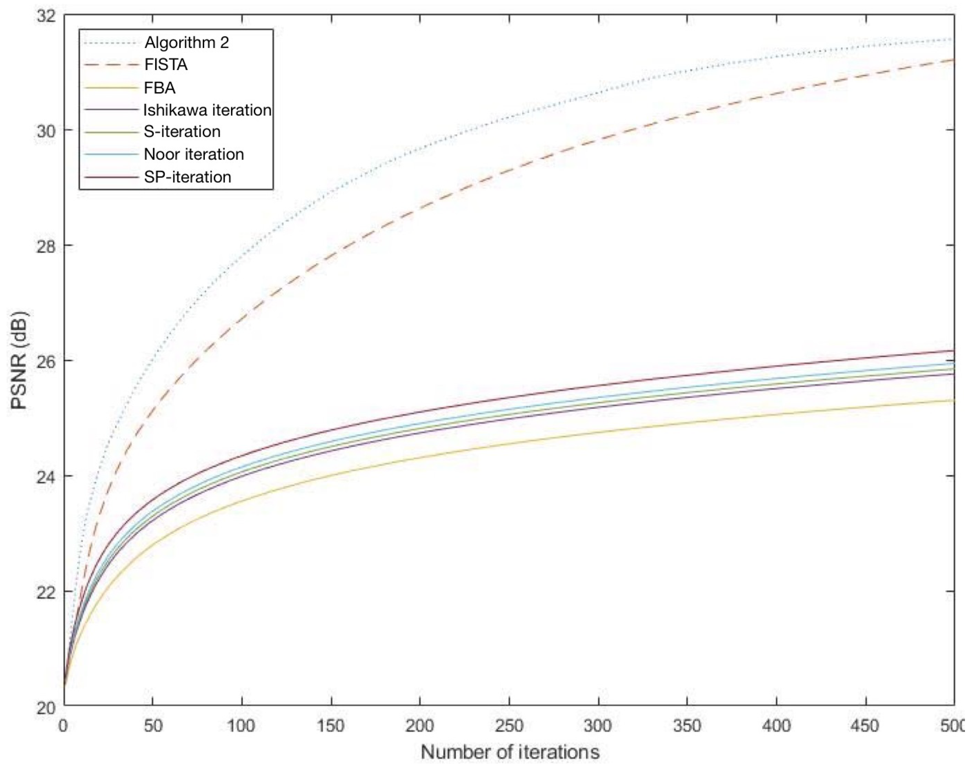
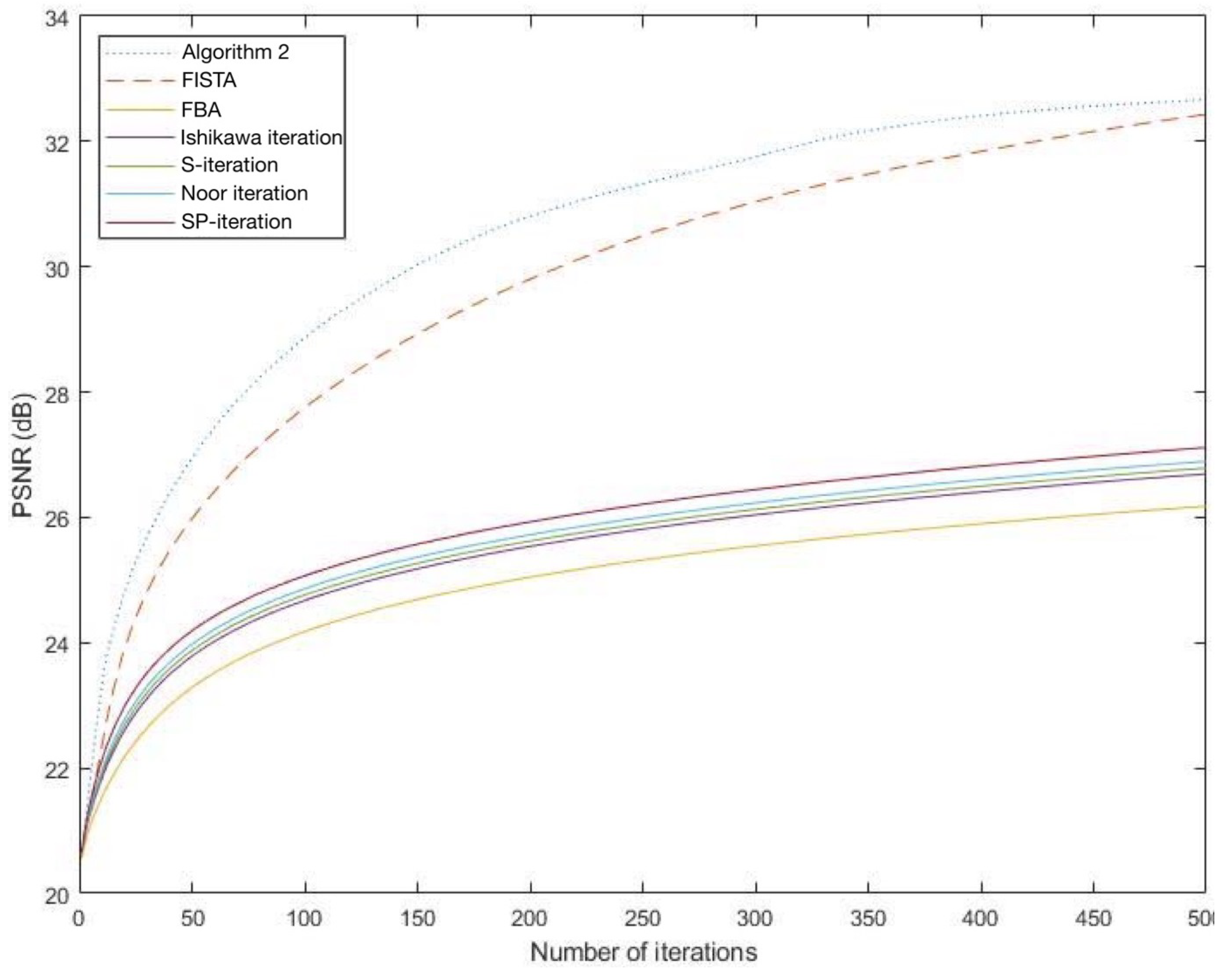
The following experiments show the efficacy of the blurring results of Suan Dok and Aranyavivek temples at the 500th iteration of Algorithms 2, FISTA, FBA, Ishikawa iteration, S-iteration, Noor iteration and SP-iteration using PSNR as our measurement, shown in tables and figures as follows.

It is observed from Figure 1 and Figure 2 that the graph of PSNR of Algorithm 2 is higher than that of FISTA FBA, Ishikawa iteration, S-iteration, Noor iteration and SP-iteration which shows that Algorithm 2 gives a better performance than the others.

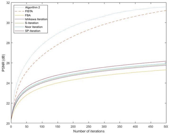
Figure 1. The graphs of PSNR of each algorithm for Suan Dok temple.

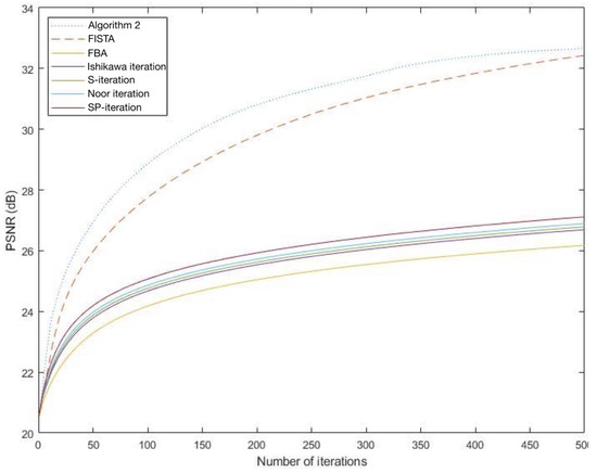
Figure 2. The graphs of PSNR of each algorithm for Aranyawiwek temple.

The efficiency of each algorithm for image restoration is shown in Table 2, Table 3, Table 4 and Table 5 for different number of iterations. The value of PSNR of Algorithm 2 is shown to be higher than that of FISTA, FBA, Ishikawa iteration, S-iteration, Noor iteration and SP-iteration. Thus, Algorithm 2 has a better convergence behavior than the others.

Table 2. The values of PSNR for Algorithm 2, FISTA, FBA of Suan Dok temple.

No. Iterations	Algorithm 2	FISTA	FBA
1	20.41801	20.36432	20.27827
5	21.56154	21.13340	20.64981
10	22.81140	22.00081	20.96027
25	24.54825	23.73266	21.56257
100	27.80053	26.71268	22.93002
250	30.21461	29.28515	23.92280
500	31.57117	31.21182	24.66522

Table 3. The values of PSNR for Ishikawa iteration, S-iteration, Noor iteration and SP-iteration of Suan Dok temple.

No. Iterations	Ishikawa Iteration	S-Iteration	Noor Iteration	SP-Iteration
1	20.41010	20.42585	20.43611	20.47630
5	21.04951	21.08759	21.12646	21.23160
10	21.54370	21.59831	21.65780	21.80965
25	22.44491	22.51817	22.59948	22.79284
100	23.98112	24.05696	24.14345	24.33880
250	24.97654	25.05383	25.14335	25.43583
500	25.75882	25.84223	25.93954	26.16025

Table 4. The values of PSNR for Algorithm 2, FISTA and FBA of Aranyawiwek temple.

No. Iterations	Algorithm 2	FISTA	FBA
1	20.62485	20.57077	20.48543
5	21.85350	21.37734	20.86196
10	23.31840	22.35583	21.19050
25	25.29317	24.39293	21.85570
100	28.86437	27.75046	23.44804
250	31.32694	30.48999	24.60734
500	32.66988	32.43108	25.45769

Table 5. The values of PSNR for Algorithm 2, Ishikawa iteration, S-iteration, Noor iteration and SP-iteration of Aranyawiwek temple.

No. Iterations	Ishikawa Iteration	S-Iteration	Noor Iteration	SP-Iteration
1	20.61695	20.63272	20.64371	20.65791
5	21.28692	21.32823	21.37058	21.46923
10	21.83445	21.89601	21.96356	21.12342
25	22.87547	22.96182	22.057648	22.27264
100	24.64759	24.76190	24.86123	25.06857
250	25.81261	25.89987	26.00121	26.20981
500	26.96400	26.78725	26.89572	27.11590

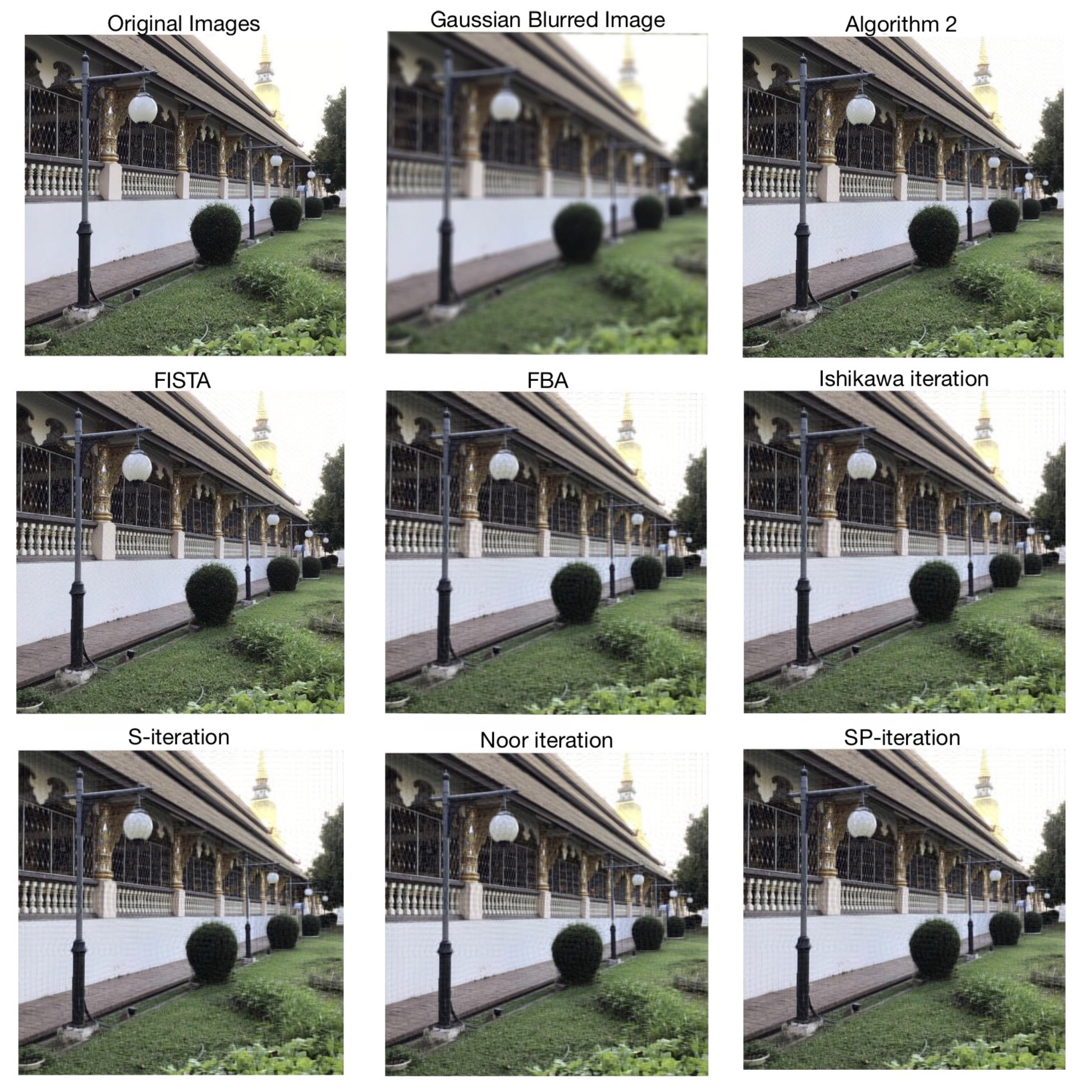
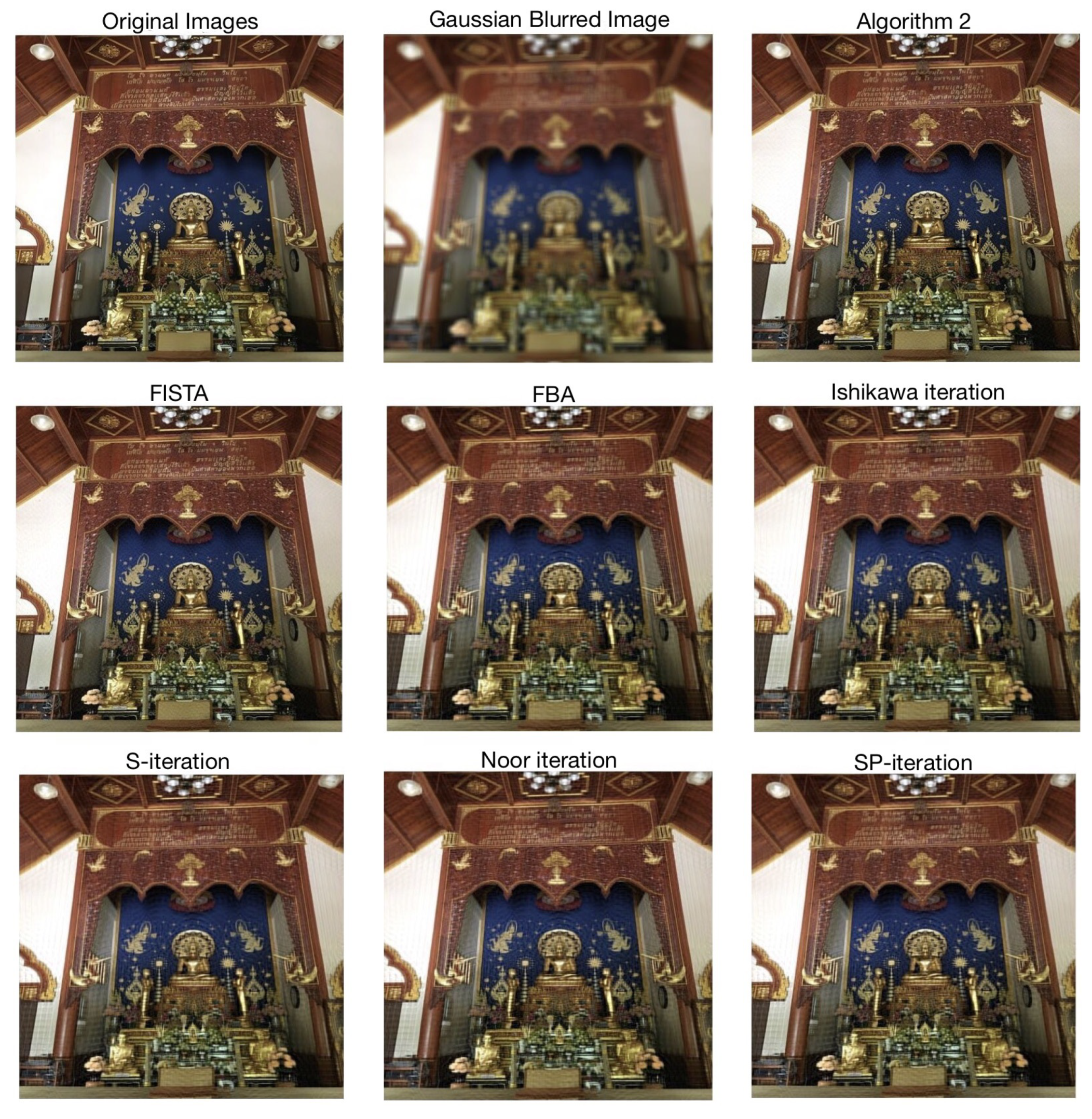
We show the original images, blurred images, and deblurred images by Algorithm 2, FISTA, FBA, Ishikawa iteration, S-iteration, Noor iteration and SP-iteration for Suan Dok (Figure 3) and Aranyawiwek temples (Figure 4).

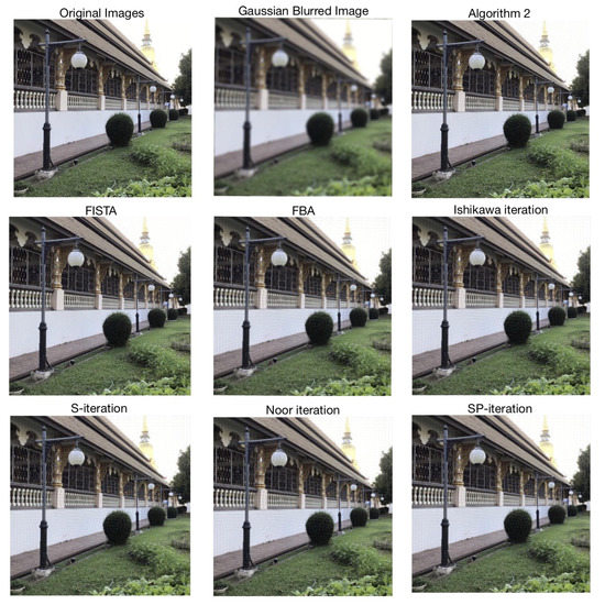
Figure 3. Results for Suan Dok temple’s deblurring image.

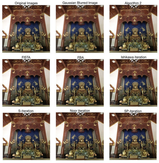
Figure 4. Results for Aranyawiwek temples’s deblurring image.

5. Conclusions

In this study, we used a coordinate affine structure to propose an accelerated fixed-point algorithm with an inertial technique for a countable family of G-nonexpansive mappings in a Hilbert space with a symmetric directed graph G. Moreover, we proved the weak convergence theorem of the proposed algorithm under some suitable conditions. Then, we compared the convergence behavior of our proposed algorithm with FISTA, FBA, Ishikawa iteration, S-iteration, Noor iteration and SP-iteration. We also applied our results to image restoration and convex minimization problems. We found that Algorithm 2 gave the best results out of all of them.

References

- Berinde, V. A Modified Krasnosel’skiǐ–Mann Iterative Algorithm for Approximating Fixed Points of Enriched Nonexpansive Mappings. Symmetry 2022, 14, 123. [Google Scholar] [CrossRef]
- Bin Dehaish, B.A.; Khamsi, M.A. Mann iteration process for monotone nonexpansive mappings. Fixed Point Theory Appl. 2015, 2015, 177. [Google Scholar] [CrossRef] [Green Version]
- Dong, Y. New inertial factors of the Krasnosel’skii-Mann iteration. Set-Valued Var. Anal. 2021, 29, 145–161. [Google Scholar] [CrossRef]
- Mann, W.R. Mean value methods in iteration. Proc. Am. Math. Soc. 1953, 4, 506–510. [Google Scholar] [CrossRef]
- Ishikawa, S. Fixed points by a new iteration method. Proc. Am. Math. Soc. 1974, 44, 147–150. [Google Scholar] [CrossRef]
- Agarwal, R.P.; O’Regan, D.; Sahu, D.R. Iterative construction of fixed point of nearly asymptotically nonexpansive mappings. J. Nonlinear Convex Anal. 2007, 8, 61. [Google Scholar]
- Noor, M.A. New approximation schemes for general variational inequalities. J. Math. Anal. Appl. 2000, 251, 217–229. [Google Scholar] [CrossRef] [Green Version]
- Phuengrattana, W.; Suantai, S. On the rate of convergence of Mann, Ishikawa, Noor and SP-iterations for continuous functions on an arbitrary interval. J. Comput. Appl. Math. 2000, 235, 3006–3014. [Google Scholar] [CrossRef] [Green Version]
- Jachymski, J. The contraction principle for mappings on a metric space with a graph. Proc. Am. Math. Soc. 2008, 136, 1359–1373. [Google Scholar] [CrossRef]
- Aleomraninejad, S.M.A.; Rezapour, S.; Shahzad, N. Some fixed point result on a metric space with a graph. Topol. Appl. 2012, 159, 659–663. [Google Scholar] [CrossRef] [Green Version]
- Alfuraidan, M.R.; Khamsi, M.A. Fixed points of monotone nonexpansive mappings on a hyperbolic metric space with a graph. Fixed Point Theory Appl. 2015, 2015, 44. [Google Scholar] [CrossRef]
- Alfuraidan, M.R. Fixed points of monotone nonexpansive mappings with a graph. Fixed Point Theory Appl. 2015, 2015, 49. [Google Scholar] [CrossRef] [Green Version]
- Tiammee, J.; Kaewkhao, A.; Suantai, S. On Browder’s convergence theorem and Halpern iteration process for G-nonexpansive mappings in Hilbert spaces endowed with graphs. Fixed Point Theory Appl. 2015, 2015, 187. [Google Scholar] [CrossRef] [Green Version]
- Tripak, O. Common fixed points of G-nonexpansive mappings on Banach spaces with a graph. Fixed Point Theory Appl. 2016, 2016, 87. [Google Scholar] [CrossRef] [Green Version]
- Sridarat, P.; Suparaturatorn, R.; Suantai, S.; Cho, Y.J. Convergence analysis of SP-iteration for G-nonexpansive mappings with directed graphs. Bull. Malays. Math. Sci. Soc. 2019, 42, 2361–2380. [Google Scholar] [CrossRef]
- Glowinski, R.; Tallec, P.L. Augmented Lagrangian and Operator-Splitting Methods in Nonlinear Mechanic; SIAM: Philadelphia, PA, USA, 1989. [Google Scholar]
- Haubruge, S.; Nguyen, V.H.; Strodiot, J.J. Convergence analysis and applications of the Glowinski Le Tallec splitting method for finding a zero of the sum of two maximal monotone operators. J. Optim. Theory Appl. 1998, 97, 645–673. [Google Scholar] [CrossRef]
- Suantai, S.; Kankam, K.; Cholamjiak, P.; Cholamjiak, W. A parallel monotone hybrid algorithm for a finite family of G-nonexpansive mappings in Hilbert spaces endowed with a graph applicable in signal recovery. Comp. Appl. Math. 2021, 40, 145. [Google Scholar] [CrossRef]
- Baleanu, D.; Etemad, S.; Mohammadi, H.; Rezapour, S. A novel modeling of boundary value problems on the glucose graph. Commun. Nonlinear Sci. Numer. Simulat. 2021, 100, 105844. [Google Scholar] [CrossRef]
- Etemad, S.; Rezapour, S. On the existence of solutions for fractional boundary value problems on the ethane graph. Adv. Differ. Equ. 2020, 2020, 276. [Google Scholar] [CrossRef]
- Hanjing, A.; Suantai, S. A fast image restoration algorithm based on a fixed point and optimization method. Mathematics 2020, 8, 378. [Google Scholar] [CrossRef] [Green Version]
- Bussaban, L.; Suantai, S.; Kaewkhao, A. A parallel inertial S-iteration forward-backward algorithm for regression and classification problems. Carpathian J. Math. 2020, 36, 21–30. [Google Scholar] [CrossRef]
- Lions, P.L.; Mercier, B. Splitting Algorithms for the Sum of Two Nonlinear Operators. SIAM J. Numer. Anal. 1979, 16, 964–979. [Google Scholar] [CrossRef]
- Janngam, K.; Suantai, S. An accelerated forward-backward algorithm with applications to image restoration problems. Thai. J. Math. 2021, 19, 325–339. [Google Scholar]
- Alakoya, T.O.; Jolaoso, L.O.; Mewomo, O.T. Two modifications of the inertial Tseng extragradient method with self-adaptive step size for solving monotone variational inequality problems. Demonstr. Math. 2020, 53, 208–224. [Google Scholar] [CrossRef]
- Gebrie, A.G.; Wangkeeree, R. Strong convergence of an inertial extrapolation method for a split system of minimization problems. Demonstr. Math. 2020, 53, 332–351. [Google Scholar] [CrossRef]
- Beck, A.; Teboulle, M. A Fast Iterative Shrinkage-Thresholding Algorithm for Linear Inverse Problems. SIAM J. Imaging Sci. 2009, 2, 183–202. [Google Scholar] [CrossRef] [Green Version]
- Verma, M.; Shukla, K. A new accelerated proximal gradient technique for regularized multitask learning framework. Pattern Recogn. Lett. 2018, 95, 98–103. [Google Scholar] [CrossRef]
- Johnsonbaugh, R. Discrete Mathematics; Pearson: Hoboken, NJ, USA, 1997. [Google Scholar]
- Tan, K.; Xu, H.K. Approximating fixed points of nonexpansive mappings by the ishikawa iteration process. J. Math. Anal. Appl. 1993, 178, 301–308. [Google Scholar] [CrossRef] [Green Version]
- Takahashi, W. Introduction to Nonlinear and Convex Analysis; Yokohama Publishers: Yokohama, Japan, 2009. [Google Scholar]
- Moudafi, A.; Al-Shemas, E. Simultaneous iterative methods for split equality problem. Trans. Math. Program. Appl. 2013, 1, 1–11. [Google Scholar]
- Nakajo, K.; Shimoji, K.; Takahashi, W. Strong convergence to a common fixed point of families of nonexpansive mappings in Banach spaces. J. Nonlinear Convex Anal. 2007, 8, 11–34. [Google Scholar]
- Bauschke, H.H.; Combettes, P.L. Convex Analysis and Monotone Operator Theory in Hilbert Spaces, 2nd ed.; Springer: Berlin, Germany, 2017. [Google Scholar]
- Combettes, P.L.; Wajs, V.R. Signal recovery by proximal forward-backward splitting. Multiscale Model. Simul. 2005, 4, 168–1200. [Google Scholar] [CrossRef] [Green Version]
- Moreau, J.J. Fonctions convexes duales et points proximaux dans un espace hilbertien. Comptes Rendus Hebd. Des Séances L’académie Des Sci. 1962, 255, 2897–2899. [Google Scholar]
- Beck, A. First-Order Methods in Optimization; Tel-Aviv University: Tel Aviv-Yafo, Israel, 2017; pp. 129–177. ISBN 978-1-61197-498-0. [Google Scholar]
- Polyak, B. Some methods of speeding up the convergence of iteration methods. USSR Comput. Math. Math. Phys. 1964, 4, 1–17. [Google Scholar] [CrossRef]
- Nesterov, Y. A method for solving the convex programming problem with convergence rate O(1/k2). Dokl. Akad. Nauk SSSR 1983, 269, 543–547. [Google Scholar]
- Vogel, C.R. Computational Methods for Inverse Problems; SIAM: Philadelphia, PA, USA, 2002. [Google Scholar]
- Eldén, L. Algorithms for the regularization of ill-conditioned least squares problems. BIT Numer. Math. 1977, 17, 134–145. [Google Scholar] [CrossRef]
- Hansen, P.C.; Nagy, J.G.; O’Leary, D.P. Deblurring Images: Matrices, Spectra, and Filtering (Fundamentals of Algorithms 3) (Fundamentals of Algorithms); SIAM: Philadelphia, PA, USA, 2006. [Google Scholar]
- Tikhonov, A.N.; Arsenin, V.Y. Solutions of Ill-Posed Problems; V.H. Winston: Washington, DC, USA, 1977. [Google Scholar]
- Tibshirani, R. Regression shrinkage and selection via the lasso. J. R. Stat. Soc. B Methodol. 1996, 58, 267–288. [Google Scholar] [CrossRef]
- Thung, K.; Raveendran, P. A survey of image quality measures. In Proceedings of the International Conference for Technical Postgraduates (TECHPOS), Kuala Lumpur, Malaysia, 14–15 December 2009; pp. 1–4. [Google Scholar]
Publisher’s Note: MDPI stays neutral with regard to jurisdictional claims in published maps and institutional affiliations. |
© 2022 by the authors. Licensee MDPI, Basel, Switzerland. This article is an open access article distributed under the terms and conditions of the Creative Commons Attribution (CC BY) license (https://creativecommons.org/licenses/by/4.0/).